APPLICATION OF BiCONJUGATE
GRADIENT STABILIZED
METHOD WITH SPECTRAL
ACCELERATION FOR
PROPAGATION OVER TERRAIN
PROFILES
A THESIS
SUBMITTED TO THE DEPARTMENT OF ELECTRICAL AND
ELECTRONICS ENGINEERING
AND THE INSTITUTE OF ENGINEERING AND SCIENCE
OF BILKENT UNIVERSITY
IN PARTIAL FULFILLMENT OF THE REQUIREMENTS
FOR THE DEGREE OF
MASTER OF SCIENCE
By
Barış Babaoğlu
October, 2003
I certify that I have read this thesis and that in my opinion it is fully adequate, in scope and in quality, as a thesis for the degree of Master of Science.
Prof. Dr. Ayhan Altıntaş (Supervisor)
I certify that I have read this thesis and that in my opinion it is fully adequate, in scope and in quality, as a thesis for the degree of Master of Science.
Asst. Prof. Vakur B. Erturk (Co-supervisor)
I certify that I have read this thesis and that in my opinion it is fully adequate, in scope and in quality, as a thesis for the degree of Master of Science.
Prof. Dr. Cevdet Aykanat
I certify that I have read this thesis and that in my opinion it is fully adequate, in scope and in quality, as a thesis for the degree of Master of Science.
Dr. Satılmış Topçu
Approved for the Institute of Engineering and Science
Prof. Dr. Mehmet Baray
iii
ABSTRACT
APPLICATION OF BiCONJUGATE
GRADIENT STABILIZED METHOD
WITH SPECTRAL ACCELERATION
FOR PROPAGATION OVER TERRAIN
PROFILES
Barış Babaoğlu
M.S. in Electrical and Electronics Engineering
Supervisors: Prof. Ayhan Altıntaş, Asst. Prof. Vakur B. Ertürk
October 2003
Using the Method of Moments (MoM) for the computation of electromagnetic radiation / surface scattering problems is a very popular approach since obtained results are accurate and reliable. But the memory requirement in the MoM to solve discretized integral equations and the long computational time of
O(N3) operation count (where N is the number of the surface unknowns) make
the method less favorable when electrically large geometries are of interest. This limitation can be overcome by using BiConjugate Gradient Stabilized (BiCGSTAB) method, a non-stationary iterative technique that was developed to solve general asymmetric/non-Hermitian systems with an operational cost of
O(N2) per iteration. Furthermore, the computational time can be improved by
the spectral acceleration (SA) algorithm which can be applied in any iterative technique. In this thesis, Spectrally Accelerated BiCGSTAB (SA-BiCGSTAB) method is processed over systems that have huge number of unknowns resulting a computational cost and memory requirement of O(N) per iteration. Applications are presented on electrically large rough terrain profiles. The accuracy of the method is compared with MoM, conventional BiCGSTAB method and Spectrally Accelerated Forward-Backward Method (SA-FBM) where available.
Keywords: Electromagnetic rough surface scattering, Method of Moments,
v
ÖZET
SPEKTRAL HIZLANDIRILMIŞ BiEŞLENİK
GRADYAN STABİL YÖNTEMİ İLE ARAZİ
KESİTLERİNDE DALGA YAYINIMI
UYGULAMALARI
Barış Babaoğlu
Elektrik Elektronik Mühendisliği Bölümü Yüksek Lisans
Tez Yöneticileri: Prof. Ayhan Altıntaş, Yrd. Doç. Vakur B. Ertürk
Ekim 2003
Ulaşılan sonuçların doğruluğu ve güvenilirliğinden dolayı, Moment Metodunun (MoM) elektromanyetik ışınım / yüzey saçınımı hesaplamalarında kullanılması oldukça popüler bir yaklaşımdır. Ancak ayrıklaştırılmış integral denklemlerinin çözülmesi için gerekli hafıza ihtiyacı ve O(N3
)’lük uzun hesaplama süresi, bu
metodu elektriksel olarak geniş geometriler söz konusu olduğunda gözden düşürmektedir.Bu limitasyon, BiEşlenik Gradyan Stabil (BiCGSTAB) yöntemi kullanarak üstesinden gelinebilir. BiCGSTAB yöntemi, genel asimetrik ve Hermisyon olmayan sistemleri, her iterasyonda O(N2
)’lik işlem sayısı yaparak
çözmek için geliştirilen durağan olmayan bir iteratif tekniktir. Bunun da ötesinde hesaplama süresi, herhangi bir iteratif yönteme uygulanabilen spektral hızlandırma (SA) algoritmasıyla geliştirilebilir. Bu tezde spektral hızlandırılmış BiCGSTAB (SA-BiCGSTAB) metodu çok fazla sayıda bilinmeyeni bulunan sistemlere tatbik edilmiş, sonuçta hesaplama süresi ve hafıza gereksinimi her iterasyonda O(N)’e düşürülmüştür. Uygulamalar elektriksel geniş pürüzlü arazi kesitleri üzerinde gösterilmiştir. Sonuçların doğruluğu MoM, olağan BiCGSTAB yöntemi ve de uygun yerlerde Spektral Hızlandırılmış İleri-Geri (SA-FBM) yöntemiyle karşılaştırılmıştır.
Anahtar Kelimeler: Elektromanyetik pürüzlü yüzey saçınımı, Moment Metodu,
vii
Acknowledgement
I would like to express my deepest gratitude to my supervisors Prof. Ayhan Altıntaş and Asst. Prof. Vakur B. Ertürk for their supervisions, suggestions and encouragement throughout the development of this thesis.
I am also indebted to Prof. Dr. Cevdet Aykanat and Dr. Satılmış Topçu, the members of my jury, accepting to read and review this thesis and for their guidance.
I would also like to thank Gökhan Moral at ISYAM, for his astonishing patience for answering my awkward questions about the FORTRAN software programming language and as well as my colleague Celal Alp Tunç for supplying significant resources for the development of this thesis.
It is a great pleasure to express my special thanks to my family who brought me to this stage with their endless patience and dedication. Finally, I would like to thank Seha, for her unconditional love and interest she has shown during all the phases of this thesis; without her, this thesis would not be possible.
Contents
1 Introduction
1.1 Propagation Prediction Models………. 1
1.2 Integral Equation Methods Based On Terrain Propagation...….…. 3
1.3 Iterative Approaches On One-Dimensional Rough Surface Scattering 4 2 Scattering Problem for 1D Rough Surfaces and Method of Moments (MoM) 2.1 Introduction...…………... 7
2.2 Electric and Magnetic Field Integral Equations...………… 8
2.2.1 EFIE for Horizontal Polarization...………. 9
2.2.2 MFIE for TE Polarization………... 12
2.3 Method of Moments (MoM) Formulation...……… 16
2.3.1 Point Matching Method...………... 16
2.3.2 Weighted Residuals for Point Matching...………. 18
2.3.3. MoM Formulation for EFIE...………. 19
2.3.4 MoM Formulation for EFIE...……….. 20
2.3.5 Solution of MoM...………... 20
3 Gradient Type of Iterative Solvers and the Spectral Acceleration (SA) Algorithm 3.1 Introduction...……… 22
3.2 Conjugate Gradient Type of Methods...………….. 24
3.2.1 Conjugate Gradient Method...……… 24
3.2.2 BiConjugate Gradient Method...…….. 27
3.3 Numerical Results for the BiCGSTAB Method...……. 31
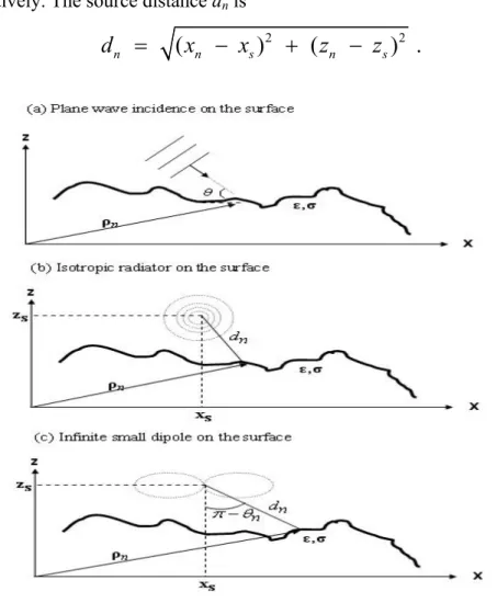
3.3.1 Source Incident on the Terrain Profile...………. 32
3.3.2 Applications of BiCGSTAB over Rough Surfaces...… 34
3.3.3 Computational Cost of BiCGSTAB...……….. 45
3.4 Spectral Acceleration Algorithm...………... 46
3.4.1 SA Algorithm for Quasi-planar Surfaces...……... 47
3.4.1.1 Spectral Acceleration for Horizontal Polarization... 48
3.4.1.2 Spectral Acceleration for Vertical Polarization... 51
3.4.1.3 Integration Contour for Quasi-planar Surfaces... 52
3.4.1.4 Integration Steps...……….. 55
3.4.1.5 Operation Count for the SA for Quasi planar Surfaces 56 3.4.2 SA Algorithm for Rough Surfaces...……….. 57
3.4.2.1 Spectral Acceleration for Horizontal Polarization... 57
3.4.2.2 Spectral Acceleration for Vertical Polarization...…. 59
3.4.2.3 Integration Path for Rough Surfaces...………. 60
3.4.2.4 Integration Steps...………. 63
3.4.2.5 Operation Count for the SA for Rough Surfaces…… 65
3.5 Numerical Results for Quasi-planar Surfaces...……… 65
4 Computation of Scattered Field on Rough Surface Profiles 4.1 Introduction...……… 78
4.2 Computation of Scattered Field with Spectral Acceleration... 79
4.3 Numerical Results for Rough Surfaces...……… 80
4.4 Computational Cost of SA-BiCGSTAB for Rough Surfaces...……. 93
5 Conclusions and Future Work……….... 96
Appendix A………... 99
Appendix B.………... 103
List of Figures
2.1 A generic terrain profile...………. 8
3.1 Pseudo code for the Conjugate Gradient method...…….. 26
3.2 Pseudo code for the Bi-Conjugate Gradient method...…………... 28
3.3 Pseudo code for the Bi-Conjugate Gradient Stabilized method...……. 30
3.4 Sources incident on the terrain profile...……… 33
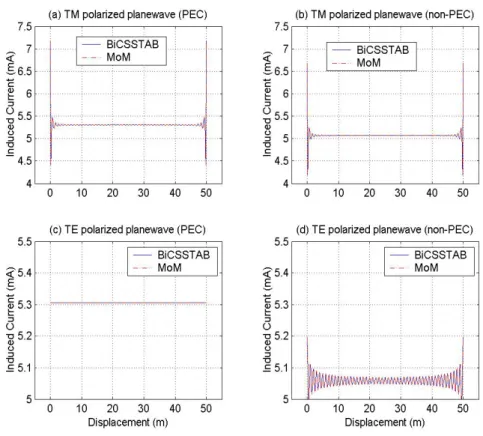
3.5 Strip surface of width 50λ...……… 34
3.6 Distributed current on a strip, oblique plane wave incidence...…….. 35
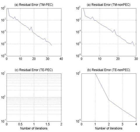
3.7 Residual errors of Figure 3.6...………. 36
3.8 Distributed current on a 100λ rough surface, grazing plane wave...…. 37
3.9 Residual errors of Figure 3.8...………. 37
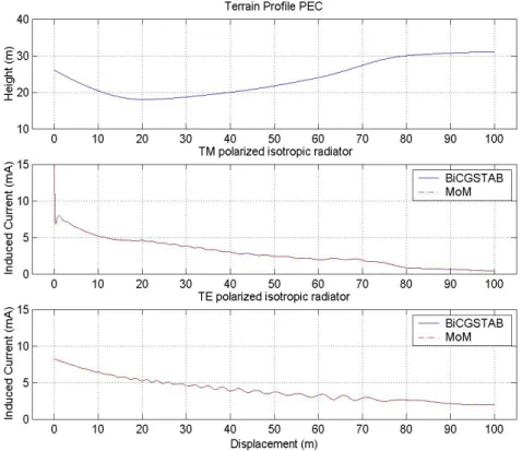
3.10 Isotropic radiator on the rough surface...……… 38
3.11 Residual errors of Figure 3.10...……….. 38
3.12 Dipole antenna on the rough surface...……….. 39
3.13 Residual errors of Figure 3.12...………. 39
3.14 Dipole antenna on the rough surface...………... 40
3.15 Residual errors of Figure 3.14...…….. 41
3.16 The ship under target...…………. 42
3.17 Current distribution on a ship (wind speed: 0m/s)...…………... 43
3.18 Current distribution on a ship (wind speed: 5m/s)...…… 43
3.19 Current distribution on a ship (wind speed: 10m/s)...………... 44
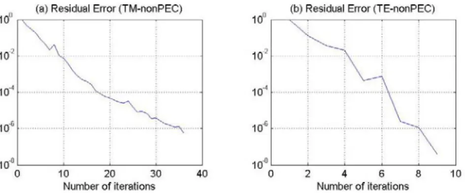
3.20 Residual error for PEC case...……… 44
3.21 Residual error for non-PEC case...……… 44
3.23 Forward and backward propagation fields on a flat surface...………. 47
3.24 Weak and strong regions for the nth receiving point at forward direction.. 48
3.25 Integration paths of Hankel function...……… 53
3.26 Generic interpretation of asymptotic lit region...……….. 53
3.27 Integrand along the SDP of a flat surface……… 54
3.28 Integration path in the complex plane...………. 61
3.29 Distributed current on a strip, oblique plane wave incidence...……….. 66
3.30 Isotropic radiator on a quasi-planar surface...………. 67
3.31 Residual errors for Figure 3.30...………. 68
3.32 Dipole antenna on a quasi-planar surface...……… 68
3.33 Residual errors of Figure 3.32...……….. 69
3.34 Plane wave on a quasi-planar surface with grazing incidence...…... 69
3.35 Residual errors of Figure 3.34...……….. 70
3.36 Dipole antenna on a quasi-planar surface...………. 70
3.37 Residual errors of Figure 3.36...………. 71
3.38 Dipole antenna on a quasi-planar surface...…………. 71
3.39 Residual errors of Figure 3.38...………... 72
3.40 Current distribution on a ship (wind speed: 0m/s)...…. 74
3.41 Current distribution on a ship (wind speed: 5m/s)...……… 74
3.42 Current distribution on a ship (wind speed: 10m/s)...………. 75
3.43 Dipole on a quasi-planar surface of width 1000λ...………... 75
3.44 Residual errors of Figure 3.43...……… 76
3.45 Dipole antenna on a quasi-planar surface...….. 76
4.1 The scattering zone of a generic terrain profile...…… 80
4.3 Difference errors for scattered fields of Figure 4.2...……... 83
4.4 Scattered fields from a 500λ width rough surface...………. 84
4.5 Difference errors for scattered fields of Figure 4.4...……. 85
4.6 Scattered fields from a 1000λ width rough surface...……….. 85
4.7 Difference errors for scattered fields of Figure 4.6...…….. 86
4.8 Scattered fields from a 1000λ width rough surface...…………. 87
4.9 Difference errors for scattered fields of Figure 4.8...………... 87
4.10 Scattered fields from a 1000λ width rough surface...……… 88
4.11 Difference errors for scattered fields of Figure 4.10...…………. 88
4.12 Scattered fields from a 2000λ width rough surface...……… 89
4.13 Difference errors for scattered fields of Figure 4.12...………. 90
4.14 Scattered fields from a 10000λ width rough surface...……..…… 91
4.15 Scattered fields from a 10000λ width rough surface...………… 91
4.16 Scattered fields from a 10000λ width rough surface...……….... 92
List of Tables
3.1 Operation count per iteration for BiCG and BiCGSTAB methods...….. 30
3.2 Storage requirements for BiCG and BiCGSTAB methods...……… 31
3.3 Computational costfor BiCGSTAB method ……...……….. 45
4.1 Study parameters...……….. 82
4.2 Study parameters...………. 89
Chapter 1
Introduction
During the past years, the mobile radio communication industry has grown enormously, powered by digital RF fabrication improvements, large-scale circuit integration and other technologies which make the mobile radio equipment smaller, cheaper but most important, reliable. Since then the study of coverage analysis and propagation losses for wireless communications has been of great interest. The radio spectrum allocation is the basis of RF communications, and it is closely tied to coverage analysis, computation of interference and propagation losses.
In this regard, the accurate prediction of electromagnetic field strengths over large areas (i.e., terrain propagation) in different environments has great importance. Thus, the main problem is related to the computation of precise solution. A great number of solution techniques have been developed. The first class of these techniques is based on propagation prediction models. These are the automatic tools for radio coverage prediction over geographical databases. The second class is the integral equation based methods dealing directly with Maxwell’s equations for the computation of scattered field.
1.1 Propagation Prediction Models
These methods are focused on propagation loss and coverage analysis according to their nature. Also they are fast to apply for the investigation of scattered fields. There are three approaches for predicting field patterns, namely, empirical, heuristic and deterministic.
As the name suggests, the empirical method involves the experience of measurements. Okumura – Hata method [1] is a well known example of such approach. Empirical models interest on the geometrical data at the level of categorization. For instance, for urban, sub-urban and the rural areas, different formulae may be issued. The drawback of these methods is that they mainly focus on the field attenuation. The effects of diffraction and reflection due to obstacles in the region of interest are omitted.
Heuristic methods usually depend on high frequency asymptotic principles for the diffraction losses. Well known examples for these methods are Spherical Earth Knife–Edge algorithm [2] based on knife–edge diffraction assumption, Geometrical Theory of Diffraction (GTD) [3] using wedge diffractions including finite conductivity and local roughness effects. Since these methods require more detailed information about the environment than the empirical models, complex geometries defining the number of Knife–Edges or wedges make the usage of the methods overwhelming.
Deterministic models are issued for the simulation of radio wave propagation and are concerned with the computation of radio channel properties related with the description of geographical environment. Most of these approaches depend on ray tracing algorithms, whose computational complexity is prohibitive. Another variant of this kind of methods is a parabolic approximation to the Helmholtz equation, derived for both integral and differential forms [4]-[6]. Nevertheless parabolic approximation assumes that the propagation of the field is addressed through the forward direction. Thus, the backscattered field contribution is omitted.
One should note that there is a trade-off between the accuracy of the prediction and the computational speed in propagation models. As the precision
of the technique is increased, the order of the complexity to define the geographical area of interest also enlarges which creates long CPU times.
1.2 Integral Equation Methods Based On Terrain
Propagation
These are numerical methods dealing directly with the solution of Maxwell equations; therefore hesitation in the electromagnetic analysis would be prevented. Moreover, they can be used as a reference solution for the validation of prediction methods and to obtain the limits of these methods under certain circumstances. Many of the integral equations (IE) are based on Method of Moments (MoM) [7]. This method proceeds to find the value of each unknown (for example, current distribution on a rough surface), which is the solution of discretized problem. But when the total number of unknowns, N, is very large (dealing with electrically large surface geometries), the solution of such problem grows exponentially in terms of computational CPU time and storage requirements. Direct solution methods of the MoM, such as LU decomposition requires an operational cost of O(N3). This has led to the
development of iterative schemes to reduce computational count to O(N2).
The first application of IE based method to the terrain propagation problem can be found in [8] where an IE is applied over small terrain profiles. Nevertheless, due to computational cost associated with the number of unknowns, the application of the method on the electrically large profiles is unfeasible. A bit more improved method in terms of computational cost is proposed in [9] with some specific considerations, such as neglecting backscattering and deducing magnetic conductivity. The assumptions make the method less reliable and still time consuming. Later on, in [10] an IE formulation is used in conjunction with an iterative version of MoM known as Banded Matrix Iterative Approach (BMIA). Limited with some certain
problems, a parallel implementation of the method is applicable. However the method maintains the computation complexity.
A more efficient solution is given in [11], in which Fast Far Field Approximation (FAFFA) was introduced and modified for an IE formulation. In this approach, method succeeds in massive computational savings when compared to the previous attempts to apply surface an IE to terrain propagation problem. Until FAFFA algorithm, all previous IE methods required O(N2)
operations per iteration whereas FAFFA achieves O(N4/3) operations per
iteration.
1.3 Iterative Approaches On One-Dimensional Rough
Surface Scattering
When the problem is to evaluate the current distribution over rough surface by means of an iterative method, two different approaches have recently been followed depending on the updating estimates. In the first one, so called stationary technique, the current is updated by applying the surface boundary conditions to the scattered field with the previous iteration’s current. Forward – Backward Method (FBM) [12] is a well known technique. It sweeps the surface on the forward and backward directions to find the forward and backward contributions due to the current element located at a fixed observation point. FBM was proposed for calculating the electromagnetic current on ocean-like perfectly electric conducting (PEC) surfaces at low grazing angles. The method gives accurate results within very few iterations but the computational cost is still O(N2). Furthermore, due to its stationary nature, the method fails to
converge when the surface of interest is not ordered (reentrant surface of a ship). The second class of iterative approaches is the non-stationary techniques. These are the extensions of Standard Conjugate Gradient method [13] that were developed to solve general asymmetric/non Hermition systems and therefore do
not attempt to solve the physical multiple scattering of electromagnetic energy directly. Examples of these are given in [14] where BiConjugate Gradient Method (BiCG) is used, Generalized Conjugate Gradient (GCG) used in [15], preconditioned multi-grid Generalized Conjugate Residual (GCR) approach used in [16] and Quasi-minimum Residual (QMR) employed in [17].
All of the methods mentioned previously require an operation count of
O(N2) (except the FAFFA algorithm). Thus when they are associated to solve
very-large scale problems, the computational cost prohibits their applicability. However in 1996, Chou and Johnson [18] proposed a spectral acceleration (SA) algorithm to overcome the limitation on slightly rough large scale problems.
The algorithm accelerates the matrix-vector multiplies taking place in the iterative process and divides contributions between points in strong and weak regions. The algorithm is mainly based on a spectral representation of two-dimensional Green’s function.
This technique reduces the computational cost and memory requirements to O(N) and the Spectrally Accelerated Forward – Backward Method (SA-FBM) can be applied over electrically large surfaces. But one should note that the original implementation of spectral acceleration is utilized for slightly rough quasi-planar surfaces and may not be suitable for undulating rough geometries.
With the development of SA, the restriction on large-scale problem will no longer exist but to deal with terrain propagation with the large height deviations, a modified version of SA is proposed in [19]. This algorithm implements SA–FBM to very undulating rough surfaces and the computational cost still remains at O(N). Although the algorithm is utilized firstly for the conventional FBM, since it sweeps forward and backward directions on the surface of the scatterer, it can be used in any iterative method.
The SA algorithm was utilized in conjunction with a non-stationary technique BiCG method firstly by Valero [20] in order scattering from the strip gratings.
In this thesis, electrically large rough terrain profiles have been examined with Spectrally Accelerated Biconjugate Gradient Stabilized Method (SA-BiCGSTAB). It should be emphasized that, this sort of implementation of BiCGSTAB method has not existed in the literature yet.
One other novelty of this method is the analysis of multi-valued (reentrant) surface profiles (like a ship on the sea). The conventional stationary techniques can not solve this kind of problems. A generalized version of the FBM (GFBM) [21] was offered to deal with such problem. The method includes significant changes in the decomposition of the system interaction matrix. Because of this decomposition, the approach requires an additional work and more storage requirement at each operation, which can be overwhelming if the multi-valued section is too large. In this context, GFBM can not compete with SA-BiCGSTAB method.
In order to reach these goals, a large number of implementations of SA-BiCGSTAB over various kinds of examples are presented. To show the ability of convergence, the results are compared with MoM, BiCGSTAB, GFBM and SA-FBM, respectively.
All fields and currents in this work are considered to have a time-harmonic dependence of the form ej kω that is suppressed from the expressions. The angular frequency is ω and k is the wave number of the medium, which is assumed to be free space, above the rough surface.
Chapter 2
Scattering Problem for 1D Rough
Surfaces and Method of Moments
(MoM)
2.1 Introduction
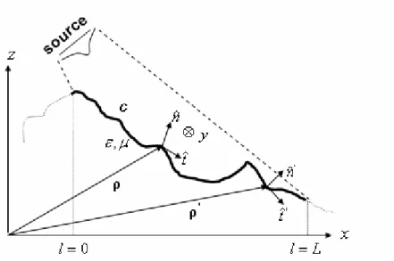
This chapter deals with the evaluation of the current distribution over a terrain profile on which an electromagnetic source is incident. To reduce the problem into two dimensions, the surface considered for such problem is assumed to have no variation along the transverse direction of the propagating field. The variation of the height at the surface along the displacement (x-axis) is characterized with the curve C and defined by z = f(x) as depicted in Figure 2.1, yielding the roughness of the surface in one dimension. The electromagnetic fields characterized by Ei(ρ) and Hi(ρ), are incident upon the surface where ρ = + x xˆ z zˆ . The terrain profile is modeled to be an imperfect conductor (with permeability µ, and permittivity є) and analyzed using an impedance boundary condition (IBC) [22]-[23] to be able to investigate more general situations.
This chapter is devoted to the discussion of integral equations in order to find current distribution on the surface of the scatterer. The formulations of integral equations are described in Section 2.2. Corresponding matrix equations to solve these integral equations are determined in Section 2.3.
Figure 2.1. A generic terrain profile.
2.2 Electric and Magnetic Field Integral Equations
The main objective of the solution of such a scattering problem is determining the physical or equivalent current distribution behavior on the surface of the scatterer. Once they are known then, the scattered fields can be evaluated by using standard radiation integrals. The method used to solve the system should be capable of finding current densities over terrain profiles accurately. This task can be achieved by an integral equation (IE) method.
In general there are many forms of integral equations. Two of the most popular examples for the time-harmonic electromagnetic fields are known as
electric field integral equation (EFIE) and magnetic field integral equation
(MFIE). The EFIE enforces the boundary condition on the tangential electric field and the MFIE enforces the boundary condition on the tangential components of the magnetic field. EFIE will be employed for horizontal polarization, namely, transverse magnetic (TM) case, and MFIE discussion will be shown for vertical polarization, namely, transverse electric (TE) case. In each case an IBC approximation will be used. The IBC implies that only the electric and magnetic fields external to the scatterer are relevant and their
relationship is a function of the material constitution (i.e., surface impedance) or surface characteristics (i.e., roughness) of the scatterer.
2.2.1 EFIE for Horizontal Polarization
Given that the IBC approximation is applied for a given scatterer shown in Figure 2.1, the total (incident plus scattered) electric field external to the surface, Et, is related as
E
t- ( .
n
ˆ
E
t) =
n
ˆ
η
s( x
n
ˆ
H
t)
, (2.1) and from the duality condition, total magnetic field Ht yieldss
1
ˆ
ˆ
ˆ
- ( .
n
) =
n
( x
n
),
η
−
t t tH
H
E
(2.2) where ηsis the surface impedance and nˆ is the unit surface normal of the terrain. The surface impedance is assumed to be constant throughout this paper but it can be easily modified if it varies along x-axis by replacing withη ρs( ). When the incident field has a horizontal polarization, (i.e., Ei = Eyˆ y), (2.1) is reduced to
E
t= (
η
sn
ˆ
x )
H
t . (2.3) The electric surface current density induced on the surface along y direction is defined as s( ) = x
n
ˆ
tJ ρ
H
(2.4) yielding (2.1)E
t=
E
i+
E
s=
η
sJ ρ
( )
(2.5) where Ei denotes the incident field and Es denotes scattered field above the scatterer. The scattered electric field is a superposition of A and F, the magnetic and electric auxiliary vector potentials, respectively [24];
=
j
ω
j
1
(
.
)
1
x
ωµε
ε
=
+
−
−
∇ ∇
− ∇
s A FE
E
E
A
A
F
(2.6)where A and F are shown to be
= ( ')
'
4
jkR Se
ds
R
µ
π
−∫∫
sA
J ρ
(2.7)= ( ')
'
4
jkR Se
ds
R
ε
π
−∫∫
sF
M ρ
(2.8) where, the prime coordinates denote the source points, S is the surface of the scatterer at the source points, Ms is the equivalent magnetic current on the surface and R is the distance from the source point to observation point given by
R
=
(
y y
−
')
2+ −
ρ ρ
' .
(2.9) Since the incident electric field is only ˆy directed, the scattered and total electric fields have only ˆy directed components which are independent of y variations (two dimensional). Therefore, the scattered electric field can be found by assuming that A has only y component which has no variations along the y-axis. Consequently, (2.6) reduces to
= x
j
ω
1
ε
−
− ∇
s
E
A
F
. (2.10) Substituting (2.7) and (2.8) into (2.10) and making the use of following relation hip between electric and magnetic currents given by
M
s=
E
tx =
n
ˆ
−
η
s( x
n
ˆ
J
s)
(2.11) which can be implied from (2.1) and (2.2), the scattered electric field is obtained as s S=
( ') ( , ')
' +
ˆ
x
( 'x ( ')) ( , ')
'
Sj
G
ds
n
G
ds
ωµ
η
−
∇
∫∫
∫∫
s s sE
J ρ
r r
J ρ
r r
(2.12)
( , ')
.
4
jkRe
G
R
π
−=
r r
(2.13) To simplify the second integral at the right hand side of (2.12), we benefit from the vector identity
∇
x(
V
ψ
) =
ψ
∇
x
V
−
x
V
∇
ψ
(2.14) Substituting (2.14) into (2.12) yields
∇
x[( 'x ) ] = G x( 'x ) +
n
ˆ
J
sG
∇
n
ˆ
J
s∇
G n
x( 'x ).
ˆ
J
s (2.15) Furthermore, the following vector identity
V V V
1x(
2x
3) =( .
V V V
1 3)
2−
( .
V V V
1 2)
3 (2.16) to expand the relationship at the first term of the right hand side of (2.14) resultsG x( 'x ) = G ( . ) ' ( . ')
∇
n
ˆ
J
s{
∇
J
sn
ˆ
− ∇
n
ˆ
J
s}
= 0
(2.17) such that the divergence of the surface current and the divergence of unit vector related with the source coordinate is equal to zero. Consequently, the second term at the right hand side of (2.15) becomes
Gx( 'x ) = ( G. ) ' ( '. G)
ˆ
ˆ
ˆ
ˆ
=
( '. G)
n
n
n
n
∇
∇
−
∇
−
∇
s s s sJ
J
J
J
(2.18)since the gradient of the Green’s function and current vector are perpendicular to each other. Thus the final expression for (2.12) is simplified to:
s C
=
( ') ( , ')
'
'
ˆ
( ') '.
( , ')
'
'
Cj
G
dy d
n
G
dy d
ωµ
ρ
η
ρ
+∞ −∞ +∞ −∞−
−
∇
∫ ∫
∫ ∫
s s sE
J ρ
r r
J ρ
r r
(2.19)where C is the terrain contour. Using the fact that 2 2 (2) 0 2 2
= (
).
j le
dl
j H
l
α βπ
αβ
β
+∞ − + −∞−
+
∫
(2.20) where H is the Hankel function of second kind and order zero, and 0(2)(2) 0 (2) s 1
=
( ')
(
' )
'
4
ˆ
ˆ
( ') '.
(
' )
'
4
C CH
k
d
k
j
n
H
k
d
ωµ
ρ
η
ρ
−
−
−
−
∫
∫
s s sE
J ρ
ρ ρ
J ρ
ρ
ρ ρ
(2.21)where H is the Hankel function of second kind of order one. Substituting 1(2)
(2.21) into (2.5), one obtains
(2) 0 (2) s 1
( |
) =
( |
)
( ')
(
' )
'
4
ˆ
ˆ
( ') '.
(
' )
'.
4
s s i y s y y C y CE
J
J
H
k
d
k
j
J
n
H
k
d
ρ ρ ρ ρωµ
η
ρ
η
ρ
= =−
−
−
−
−
−
∫
∫
ρ
ρ
ρ
ρ ρ
ρ
ρ
ρ ρ
(2.22)Equation (2.22) is referred as the electric field integral equation (EFIE) that will be used for impedance surfaces. Note that, the corresponding EFIE for a perfectly electric conducting (PEC) scatterer case can be obtained from (2.22) replacing
η
s by 0, which results
( |
) =
( ')
0(2)(
' )
'.
4
s i y y CE
ρ ρ=ωµ
J
H
k
d
ρ
−
ρ
−
∫
ρ
ρ ρ
−
(2.23)Equations (2.22) and (2.23) can be used to find the unknown current density ( ')
y
J ρ at any point on the surface of the terrain profile. Then the scattered field
can be computed via this current density.
2.2.2 MFIE for TE Polarization
For the transverse electric case, (i.e.,
H
i = yˆ Hy) since the incident magnetic field is directed along the ˆy direction, the current induced on the surface hasonly a component which is tangential to C. That is,
On the surface of the terrain the current density, related to the incident and scattered fields for the geometry of Figure 2.1, can be written as:
C C C y C C y C C
ˆ
ˆ
| =
( )| = x(
+
)|
ˆ
ˆ
ˆ
= x
|
x
|
ˆ
ˆ
=
| + x
| .
st J
tn
n y H
n
t H
n
+
−
i s s sJ
ρ
H H
H
H
(2.25)Since left and right sides of (2.25) have only tangential components, the second term at the right hand side of the (2.25) must have a tangential component. So (2.25) can be written as
J
s| =
C−
H
y| + .[ x
Ct n
ˆ ˆ
H
s| ].
C (2.26) Similar to the scattered electric field, the scattered magnetic field can be written as a superposition of magnetic and the electric auxiliary vector potentials A andF, respectively
=
1
x
j
ω
j
1
(
.
)
.
µ
ωµε
=
+
∇
−
−
∇ ∇
s F AH
H
H
A
F
F
(2.27)Since the scattered magnetic field has only a y component, the scattered and total magnetic fields have y components which are independent of y variations (two dimensional). Therefore the scattered field can be found by expanding (2.27), assuming F has only a y component which does not have a y variation, (2.27) reduces to
= x
1
j
ω
.
µ
∇
−
s
H
A
F
(2.28) Expanding (2.28) in terms of induced surface currents, the scattered magnetic field is obtained as s Sˆ
= x
( '
( ')) ( , ')
'
ˆ
ˆ
+
[ ' x ( '
( '))] ( , ')
'.
t S tt J
G
ds
j
n
t J
G
ds
ρ
ωεη
ρ
∇
∫∫
+
∫∫
sH
r r
r r
(2.29)ˆ
ˆ
x
( '
t( ')) ( , ')
' =
( '
t( ')) x [
( , ')]
'
S S
t J
G
ds
t J
G
ds
∇
∫∫
ρ
r r
−
∫∫
ρ
∇
r r
(2.30)where G(r , r’) is the Green’s function given by (2.13). To find the tangential component of the scattered field for the boundary condition in (2.26), the explicit expression is given by
s S
ˆ
.[ x
ˆ
] =
( ') .{ x[ 'x ' ( , ')]}
ˆ
ˆ
ˆ
'
ˆ
ˆ
ˆ
ˆ
+
.{ x[ ' x ( '
( '))]} G( , ')
'.
t S tt n
J
t n
t
G
ds
j
ωεη
t n
n
t J
ρ
ds
−
∫∫
∇
+
∫∫
sH
ρ
r r
r r
(2.31) Substitutingt
ˆ
' =
−
n
ˆ
' x
y
ˆ
to evaluate dot and cross products of the first term of at the right hand side of (2.31), one obtains
ˆ
ˆ
ˆ
ˆ
ˆ
ˆ
ˆ
.{ x [ ' x
]} =
.{ x [(
' x ) x
]}
ˆ ˆ
ˆ ˆ
ˆ ˆ
=
.{ x [
( ' .
)
'( .
)]}
ˆ ˆ
ˆ ˆ
=
.{ x [
( ' .
)]}
ˆ ˆ ˆ
ˆ
=
. ( ' .
) =
' .
.
t n
t
G
t n
n
y
G
t n
y n
G
n y
G
t n
y n
G
t t n
G
n
G
−
∇
−
−
∇
−
−
∇
+
∇
−
−
∇
−
∇
−
∇
(2.32)Note that the gradient of the Green’s function and the ˆy directed unit vector are perpendicular to each other. Furthermore, dot and cross products of the second term of at the right hand side of (2.31) are treated as follow;
ˆ
.{ x[ ' x ']} = .{ ' ( . ')
ˆ
ˆ
ˆ
ˆ
ˆ
ˆ
ˆ
' ( . ')}
ˆ
ˆ ˆ
ˆ
ˆ
ˆ ˆ
= .{ ' ( . ')} = -1.
t n
n
t
t n n t
t
n n
t
t
n n
−
−
(2.33)Where C is the contour of the terrain, substituting results of (2.32) and (2.33) into (2.31) results in s
ˆ ˆ
.[ x
] =
( ') '.
ˆ
( , ')
'
'
( ') ( , ')
'
'.
t C t Ct n
J
n
G
dy d
j
J
G
dy d
ρ
ωεη
ρ
+∞ −∞ +∞ −∞−
∫ ∫
∇
−
∫ ∫
sH
ρ
r r
ρ
r r
(2.34)(2) 1 (2) s 0
ˆ
.[ x
ˆ
] =
( ') '.
ˆ
ˆ
(
' )
'
4
( ')
(
' )
'.
4
t C t C
k
t n
j
J
n
H
k
d
J
H
k
d
ρ
ωεη
ρ
−
−
−
−
∫
∫
sH
ρ
ρ
ρ ρ
ρ
ρ ρ
(2.35)If we substitute (2.35) into (2.26) and rearrange it, we obtain (2) 1 (2) s 0
ˆ
ˆ
( |
) =
( |
)
( ') '.
(
' )
'
4
+
( ')
(
' )
',
4
s s i y t t c t ck
H
J
j
J
n
H
k
d
J
H
k
d
ρ ρ ρ ρρ
ρ
ωεη
ρ
= =−
+
−
−
∫
∫
ρ
ρ
ρ
ρ ρ
ρ
ρ ρ
(2.36)Equation (2.36) is referred as the magnetic field integral equation (MFIE) for impedance surfaces. Note that, the corresponding MFIE for a perfectly electric conducting (PEC) scatterer case can be obtained from (2.36) replacing
η
s by 0, which results (2) 1ˆ
ˆ
( |
) = ( |
)
( ') '.
(
' )
'.
4
s s i y t t ck
H
ρ
ρ ρ=J
ρ ρ=j
J
n
H
k
d
ρ
−
ρ
+
∫
ρ
ρ
ρ ρ
−
(2.37)Equations (2.36) and (2.37) can be used to find the unknown current density ( ')
y
J ρ at any point on the surface of the terrain profile. Then the scattered field
can be computed via this current density.
Solution of the integral equations (2.22) and (2.36) to find unknown currents is not analytically possible. Therefore, a method of moments (MoM ) solution has been developed for the investigation of the induced current, as explained in the following chapter.
2.3 Method of Moments (MoM) Formulation
Although the terrain C has an arbitrary extension, the incident field on the surface is considered to be finite so that the illuminated rough surface and, consequently the integration in equations (2.22) and (2.36) can be confined to a finite region of length L. Thus, these equations can be solved by using a
numerical technique called method of moments (MoM). In this thesis, MoM is used in conjunction with the point matching technique. The surface of the scatterer is divided into N segments. Then, unknown current distribution on the scatterer surface is expanded in N terms of basis functions, forming N unknown current coefficients. Each current coefficient is associated with a segment of the scatterer surface. Therefore, at a fixed observation point due to the incident field, one obtains a single equation with N unknowns. Then enforcing the field at each observation point on the surface, N linearly independent equations are found. Consequently, the integral equation is transformed into a linear system equation which is easier to be solved.
2.3.1 Point Matching Method
The EFIE in (2.22) and the MFIE in (2.36) are solved for the unknown surface current density Js(ρ’) using MoM procedure. Namely, first the surface current density is expanded in terms of a finite series of the form of
1
( ') =
( ')
N s m m mJ
I g
=∑
ρ
ρ
(2.38)where gm(ρ’) represents each known basis (expansion) function and Im is the
unknown coefficients of this basis function to be determined at the end of MoM procedure When (2.38) is substituted into (2.23) or (2.36) for a nth observation point on the scatterer surface;
1 1 1 (2) , 1 2 0 (2) 3 1 ( ) ( ') ( ')
( )|
=
( |
|)
'
ˆ
ˆ
'.
(|
|)
'
N N m m m m m m N m m m i y T E H m C m C I g I g I gT
c
c
H
k
d
c
n
H
d
ρ
ρ
= = = =−
+
−
+
−
∑
∑
∑
∫
∫
ρ ρ ρρ
ρ ρ
ρ
ρ ρ
(2.39)where c1= −ηs, / 4 c2 = −ωµ and c3 = − jkηs/ 4 for the EFIE. And for the MFIE, c1= ηs, / 4 c2 = ωεηs and c3= jk/ 4. Expression given by (2.39) can be illustrated in general as
1
= (
)
N m m mv
I F g
=∑
(2.40) where 1 1 1 , (2) 1 2 0 (2) 3 1 ( ) ( ') ( ')=
( ) |
(
) =
( |
|)
'
ˆ
ˆ
'.
(|
|)
'.
N N m m m m N m m i y T E H m m C m C g g gv
T
F
c
c
H
k
d
c
n
H
d
ρ
ρ
ρ
= = = =−
+
−
+
−
∑
∑
∑
∫
∫
ρ ρ ρρ
ρ ρ
ρ
ρ ρ
(2.41)In (2.41), F is called as the linear integral operator, gm is the response
function and v is the excitation function. A numerical solution of (2.41) for a single observation point ρ = ρn leads to one equation with N unknowns. If we repeat this N time by choosing N observation points, we have a system of N linear equations with N unknowns. Since this linear system was derived by applying boundary conditions at N discrete points, the technique is called as the
point matching method. To improve the point matching method solution, a
vector inner product can be defined as: *
S
,
=
.
ds
,
〈
w g
〉
∫∫
w g
(2.42) where * is the conjugate of a vector, w is the weighting functions and S is the surface of the structure to be analyzed. This weighting factor of basis functions is a better approximation instead of single point matching method.2.3.2 Weighted Residuals for Point Matching
The point matching method enforces the electromagnetic boundary condition only at discrete points. Between these points the boundary conditions may not be satisfied so that a residual error may occur between the exact boundary condition and the one found by point matching method. To minimize this residual, the method of weighted residuals is utilized in conjunction with the inner product in (2.42). This technique is called the method of moments
(MoM). MoM forces the boundary conditions to be satisfied in average sense over the entire surface. To achieve this situation, we define a set of N weighting functions {wn}= w1, w2, …… wN in the domain of the operator F. If we take the
inner products between each side of (2.38),
1
, =
, (
)
1, 2,...
N n m n m mw v
I w F g
n
N
=〈
〉
∑
〈
〉
=
(2.43) In this thesis a set of Dirac delta weighting functions, i.e., (δ p p− n) where p is a position with respect to origin and pn is the point at which the boundary condition is enforced, is used to reduce number of required operations (integrals coming from vector inner product). When we utilize these weighting functions in (2.40) and use (2.42) as the inner product, (2.40) becomes1 1 1
(
), =
(
) , (
)
1, 2,...
(
)
=
(
) (
)
1, 2,...
|
(
) |
1, 2,... .
n n N n m n m m N n m n m m S S N p p m m p p mp p v
I
p p
F g
n
N
p p v ds
I
p p F g
ds n
N
v
I F g
n
N
δ
δ
δ
δ
= = = = =〈
−
〉
〈
−
〉
=
−
−
=
=
=
∑
∑
∫∫
∫∫
∑
(2.44) So we deal with only the remaining integrations whose specified by F(gm) inequation (2.41).
2.3.3 MoM Formulation for EFIE
The set of N equations in (2.41) may be written in the matrix form of,
Z I
. =
V
(2.45) where Z is the impedance matrix. V is the excitation vector due to electromagnetic source at the match points whose elements are given byFor the linear integral operator F, if we use pulse basis function which can be denoted as:
( ') =
{
1 ' 0 elsewhere th m segment mg
ρ
ρ ∈ (2.47) than the impedance matrix elements in (2.45), for nth receiving (observation) and mth source points pair, can be approximated as [19]m (2) m (2) ' 0 1 2 1 ln = 4 4 2 ˆ ˆ ( | |) ( | |) . . 4 4 m m n m m m n m m nm k x j x n m e nm k H k x j x H k n n m
Z
γ
ωµ
η
π
ωµ
η
ρ
∆ ⎡ ⎛ ⎞⎤ − ⎢ − ⎜ ⎟⎥∆ − ⎝ ⎠ ⎣ ⎦ − − ∆ − ∆ − ≠⎧
⎪⎪
≅ ⎨
⎪
⎪⎩
ρ ρ ρ ρ (2.48) where 1.7811γ = is the Euler constant , e is equal to 2.728, ∆xm is the distancebetween two consecutive source points (segment width) and ηm is the surface impedance at the point ρm. Off-diagonal matrix impedance entries can also be represented by the two dimensional Green’s function, i.e.,
nm
(
n,
m)
m+
m m(
n,
m)
mG
Z
j
G
x
x
n
ωµ
η
∂
≅ −
∆
∆
∂
ρ ρ
ρ ρ
(2.49) where (2) 0(
)
(
,
)
4
n m n mH
k
G
j
−
=
ρ
ρ
ρ ρ
(2.50) and the second term at the right hand side of (2.49) is partial derivative of the Green’s function due to the normal vector at the source point.Consequently, we transform the EFIE in (2.22) into a linear system equation given in (2.45) by the help of MoM.
2.3.4 MoM Formulation for MFIE
If we follow the same procedure for the MFIE in (2.36), by enforcing the field at the N match points and expanding the current in terms basis functions, we transform (2.36) to a linear system equation as given in (2.45) where the elements of the excitation vector V are
v
n= (
−
H
iyρ
n).
(2.51) By employing pulse basis function, the impedance matrix entries will be [19]m (2) (2) ' m 0 1 2 1 1 ln + = 4 4 2 ˆ ˆ ( | |) ( | |) . . 4 4 m m n m m m n m m nm k x j x n m e nm k H k x j x H k n n m
Z
γ
ωεη
π
ωεη
ρ
∆ ⎡ − ⎛ ⎞⎤∆ ⎜ ⎟ ⎢ ⎝ ⎠⎥ ⎣ ⎦ − ∆ + ∆ − ≠⎧
⎪⎪
≅ ⎨
⎪
⎪⎩
ρ ρ ρ ρ (2.52) Alternatively, the off-diagonal entries of the impedance matrix can be represented by the two-dimensional Green’s function,nm m
(
n,
m)
m m(
n,
m)
mG
Z
j
G
x
x
n
ωεη
∂
≅
∆
− ∆
∂
ρ ρ
ρ ρ
(2.52)2.3.5 Solution of MoM
Once the impedance matrices given with the entries (2.48) for TM polarization and (2.52) for TE polarization are formed, the linear system equation in (2.45) should be solved for unknown current coefficients I = {Im }. The direct solution methods like Gaussian elimination and LU decomposition requires a computational cost of O(N3) where N is the number of unknowns. Hence, as the dimension of the problem gets larger, computational requirements of the MoM increases very rapidly. Nevertheless, less time consuming alternative methods are available to solve these linear system equations. These methods are called iterative methods resulting an operation count of O(N2) per
iteration. One of the variants of iterative processes named Gradient type of methods, is explained in Chapter 3.
Chapter 3
Gradient Type of Iterative Solvers
and the Spectral Acceleration (SA)
Algorithm
3.1 Introduction
The primary factor limiting the use of MoM in the calculation of electromagnetic scattering from rough surfaces is that a linear system equation must be solved to obtain currents induced on the scatterer. Direct solution methods such as LU decomposition require O(N3) operations, where N is the
number of unknowns in the discretized representation of the surface current. Electrically larger scattering surfaces (for very large N) increase the computational cost of the method and make it intractable especially at high frequencies.
Using iterative techniques, computational cost is reduced to O(N2)
operations per iteration. The basic will of an iterative process is to reach to the exact solution by updating estimates at each iteration. Two different approaches can be applied as iterative schemes to solve this system equation formed by MoM. These are, namely, stationary and non-stationary iterative techniques. In each of the method, different update schemes are used for the estimates to find the exact solution.
A method is called stationary if the rule to determine the estimates at each iteration does not change from iteration to iteration (i.e. the iteration matrix is stable during the process). In stationary iterative techniques, the surface current is approximated by physical optics approximation applied to the incident field [25]. The current is then updated by applying surface boundary condition. Kapp and Brown[26] and Holliday et al. [12] choose the ordering of the updates to follow multiple scattering paths on the surface. This led Kapp and Brown and Holliday et al. to name their approaches as method of ordered multiple interactions (MOMI) and forward backward method (FBM), respectively. Such two techniques have shown a very effective and rapid convergence activities to solve linear system equations constructed by MFIE in vertical polarization case and EFIE in horizontal polarization case for the PEC and non-PEC surfaces which are single valued and rough in one dimension. But when the ordering of the scatterer is multi-valued (reentrant surfaces), divergence problem occur.
Non-stationary techniques are the second kind of iterative methods used to solve systems formed by MoM solution. These methods are extensions of standard conjugate gradient (CG) method [13] which converge to the exact solution assuming infinite precision by constructing orthogonal vector sequences. Examples are given by bi-conjugate gradient (BiCG) method used in [14] generalized conjugate gradient (GCG) method [15] and quasi-minimum residual (QMR) method [17] are some typical examples. These methods are developed to solve asymmetric/non-Hermitian complex linear systems and hence, their algorithms are different than those of stationary methods. In these kinds of methods, the rule to determine the estimates changes from iteration to iteration. The rule is based on orthogonality conditions in the space defining the linear system equation. Consequently, a new iteration matrix is generated at every iteration step to update the estimates.
This chapter is devoted to the discussion of gradient type methods and an acceleration algorithm which can be applied on such methods. The properties of conjugate gradient type methods are presented in Section 3.2. Numerical results for BiCG Stabilized methods are given in Section 3.3. The acceleration algorithm’s assets are exhibited in Section 3.4.
3.2 Conjugate Gradient Type Methods
All of these methods explained below are assumed to solve a linear system given by Ax b . Here A is a NxN interaction matrix, b is a response = vector for the system and x is the unknown vector to be solved.
3.2.1 Conjugate Gradient Method
Being the oldest and best known nonstationary technique, the conjugate gradient method is an effective method for symmetric positive definite systems. The process, which stimulates the method is the generation of vector sequences of iterates (i.e., consecutive approximations to the solution), creating residuals that correspond to the iterates, and search directions that are used to update the iterates and residuals. Although the length of these sequences can become large, only a small number of vectors are needed to be kept in memory. In order to calculate update scalars that are defined to assure that the sequences fulfill certain orthogonality conditions, there are two inner products to be used at each iteration of the method. These conditions guarantee on a symmetric positive definite linear system that the distance to the true solution is minimized according to some standards.
The iterates x(i) are updated in each iteration by a multiple αi of the search direction vector p(i):
( )i ( 1)i
( )i i
α
−=
+
x
x
p
(3.1)Correspondingly the residuals r( )i = - b A x( )i are updated as, ( )i ( 1)i
( )i i
α
−=
−
r
r
q
(3.2) where ( )i=
( )i.
q
Ap
(3.3)The choice αi = r( 1)i− Tr( 1)i− / p( )iT Ap minimizes over all possible ( )i
choices for α. The search directions are updated using the residuals ( )i ( 1)i
1 ( 1)i i
β
− − −=
+
p
r
p
(3.4) where the choice
β
i= r r
( )iT ( 1)i−/
r
( 1)i− Tr
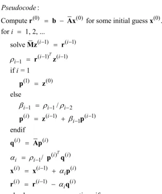
( 1)i− (3.5) ensures that p( )i and Ap( )i (or equivalently r(i) and r(i-1)) are orthogonal. In fact, one can show that this choice of βi makes p(i) and r(i) orthogonal to all previous Ap and r( )j (j) respectively.As can be seen in the Figure 3.1, in the pseudo code [13] is given for the preconditioned conjugate gradient method, there is a preconditioner M . Preconditioners are very commonly used matrix forms which enhance the condition number of the original matrix A , thus generally reducing the number of iterations to converge to the solution of the linear system. But to construct a good preconditioner matrix which can improve the iterative technique by means of iteration, the effort in terms of computational cost is increased. For M I = (where I is the identity matrix), one takes the unpreconditioned version of the conjugate gradient algorithm. In that case, by omitting the "solve" line and replacing z(i-1) by r(i-1) (and z(0) by r(0)), the algorithm may be further simplified. In this thesis, unpreconditioned versions of conjugate type methods are used because as it will be explained in Chapter 3.3, there is no need to store interaction matrix. Thus, it will be unnecessary to use a preconditioner matrix.
(0) (0) (0) ( 1) ( 1) ( 1) ( 1) 1 (1) (0) 1 1 :
Compute for some initial guess . for 1, 2, ... solve if = 1 else / T i i i i i i i i Pseudocode i i ρ β ρ ρ − − − − − − − = − = = = = = r b Ax x Mz r r z p z 2 ( ) ( 1) ( 1) 1 ( ) ( ) ( ) ( ) 1 ( ) ( 1) ( ) ( ) ( 1) ( ) endif /
check convergence; continue if necessary end T i i i i i i i i i i i i i i i i i i β α ρ α α − − − − − − − = + = = = + = − p z p q Ap p q x x p r r q
Figure 3.1 Pseudo code for the Conjugate Gradient method
The unpreconditioned conjugate gradient method creates the ith iterate
x(i) as an element of (0)
span {
+
(0),...,
( 1) (0)i−}
x
r
A
r
(3.6) so that ( ) ( )(
i)
T(
i)
e e−
−
x
x
A x
x
(3.7)is minimized, where xe is the exact solution of Ax b= . The existence of this minimum can be assured in general only if A is symmetric positive definite. Since the interaction matrices formed by MoM solutions in Chapter 2 are not positive definite, CG method is ineffective for our problem type. There are many variants of iterative techniques, which can handle linear system equations formed by the method of moments solution. These methods come out from the same origin. They depend on constructing orthogonal vector sequences which will be used to update the estimates for the next iteration.