Robust sampled data control

з ^ о в и з т SAMFIMB В Ш А СОЖ й'Ш Х,

■., 'Г -*·^ ·'< ·* .Τ’Γ*· !^Τ': ■ :·· Τ ·“^\ ^’«5^ V'*'^f t i,'!r r i:·^, '?.■;« i f

5

-Γί·^^·'* fr -:

7

ı ·.■*·fV^^*···■•”*'f•f^i'^Tr**’';····'·/ '*«r^ 4t4 i-ÍhL w-w e iM· > —< ·«» . *Ji..v«>. »İ. MR Mta V ' г‘-':-5Г'··:;' .' ‘·. ■"? '·^ “''.'.'«Ч. ■'.i·.''·»»;· < ? 4 • < Ш

/ э э ©

R O B U ST SAM PLED DATA CONTROL

A THESIS

SUBMIT ! i !) TO THE DEPARTMENT OF ELECTRICAL ENGINEERING

A N i) Mi !■: INSTITUTE OF GRADUATE STUDIES OF BILKENT UNIVERSITY

IN PAITIN AI, I'ULFILMENT OF THE REQUIREMENTS FOR THE DEGREE OF

M ASTER OF SCIENCE

By

OGAN OCALI June , 1990

Q h

•033

Ί930

I certify that I have read this thesis and that in my opinion it is fully adequate, in scope and in quality, as a thesis for the degree of Master of Science.

Prof. Dr. M. Erol Sezer(Principal Advisor)

I certify that I have read this thesis and that in my opinion it is fully adequate, in scope and in quality, as a thesis for the degree of Master of Science.

Assoc Prof. A. Bülent Özgüler

I certify that I have read this thesis and that in my opinion it is fully adequate, in scope and in quality, as a thesis for the degree of Master of Science.

Approved for the Institute of Engineering and Sciences:

Prof. Dr. Mehmet

Director of the Institute of Engineering and Sciences:

Contents

1 INTRODUCTION

1

2 ROBUST SAMPLED-DATA CONTROL OF SINGLE IN­

PUT SYSTEMS

4

2.1

System and Controller Structure... 4

2.2

Structure of $(T')

8

2.3 Stability A n alysis'... 11

2.4 An E x a m p le ... 15

3 ROBUST DECENTRALIZED SAMPLED-DATA CON­

TROL OF INTERCONNECTED SYSTEMS

19

3.1 Interconnected Systems and Decentralized C on trol...19

3.2 Expansion of The S y s t e m ...

22

3.3 Structure of $ ( i ) ... 24

3.4 Stability Analysis ... 27

4.1 Multirate Decentralized C o n t r o l... 30 4.2 Stability Analysis ... 33

4 MULTIRATE ROBUST SAMPLED-DATA CONTROL

30

ABSTRACT

ROBUST SAMPLED DATA CONTROL

Ogan Ocali

M.S. in Electrical and Electronics Engineering Supervisor: Prof. Dr. M. Erol Sezer

June, 1990

Robust control of uncertain plants is a major area of interest in control theory. In this thesis, robust stabilization of plants under a class of structural perturbations using sampled-data controllers is considered. It is shown that : 'Mi,reliable system under bounded perturbations that satisfy matching litions can be stabilized using high-gain sampled-data control, provided . i' I he sampling period is sufficiently small. This result is then applied to I - :

>1

stabilization of interconnected systems using decentralized sampled- ■ i.! ■ control, where both single-rate and multi-rate sampling schemes are ' c: :idered.

Keywords: Robust Stability, Sampled-Data Control, Additive Perturbations, Interconnected Systems, Multirate Sampling, Matching Condition.

ÖZET

ÖRNEKLENMİŞ VERİ İLE GÜRBÜZ KONTROL

Oğan O cali

Elektrik ve Elektronik Mühendisliği Bölümü Master Tez Yöneticisi: Prof. Dr. M. Erol Sezer

Haziran, 1990

Belirsiz sistemlerin

alanıdır. Bu tezde yapısal b< geribeslemesi ile gürbüz ka.r.ı; sonlu olduğu ve uyum kuanı yüksek kazançlı örneklenmi.;- sağlanabileceği gösterilmiştir, ayrışık denetim probleminede hızlarında gürbüz kararlılığı edilmiştir.

kontrolü kontrol teorisinin geniş bir ilgi liısizliği olan sistemlerin örneklenmiş durum !;l.sşlırılması incelenmiştir. Sistem belirsizliği silil (rriatching condition) sağladığı zaman, veri geribeslemesi ile gürbüz kararlılığın Bu sonuç, bazı tür bileşik sistemlerin genelleştirilerek, tekli ya da çoklu örnekleme sağlayan, a.yrışık geribesleme yapısı elde

Anahtar Sözcükler: Gürbüz Kararlılık; Örneklenmiş Veri ile Kontrol; Ayrışık Kontrol.

ACKNOWLADGEMENT

I would like to express my immeasurable gratitude to Prof. Dr. M Erol Sezer for the invaluable guidance, encouragement and above all, for the enthusiasm which he inspired on me during the study.

My thanks are due to all the individucils who made life easier with their suggestions.

List of Figures

2 .1

...16 2 . 2 ... 17 2 . 3 ... 17 2 . 4 ... 18 IX

Chapter 1

INTRODUCTION

In all control applications, because of some practical and theoretical reasons the plant that is to be controlled is not completely certain. For some cases, those uncertainties can be modelled as additive perturbations to a completely known nominal system. Due to both physical reasons and our method of modelling we may have a priori information about the structure and/or the bounds of these interconnections.

It is known that a large class of uncertain systems can be robust stabilized by high gain-continuous time feedback. Systems under perturbations which satisfy the so called matching conditions are included in this class [

8

], where the effect of perturbations can be beaten by designing the controllers to make the nominal system highly stable.

The aim of this thesis is to investigate the same problem for sampled- data control systems. Assuming that the perturbations satisfy the matching conditions, we try to answer the following questions: Can robust stability be achieved by sampled-data control? In the case of decentralized sampled-data control of interconnected systems, does multirate sampling change the nature of the problem?

The problem with sampled-data control is that the controller operates open-loop betw'een the sampling instants. In other words, the controller

is unaware of the errors that are generated by perturbations between the sampling instants, and has to wait until the next sampling instant to accommodate for those errors.

In all practical sampled-data control applications it is desirable to have large sampling periods. When the controller is a digital computer, it must be given enough time between the sampling instants for the necessary data processing. More frequent sampling requires faster and more expensive hardware. It may even be a practical impossibility to design hardware for a very fast sampled-data controller. On the other hand, as the plant to be controlled becomes more uncertain, faster correction action is needed, which necessitates more frequent sampling. If it is is possible to stabilize a plant with continuous-time feedback, one expects to find a sampling period for which a sampled-data controller exists, which achieves robust stability. An extensively general problem could be stated as follows: Given a plant uncertainty set Su, and a set of allowable sampled-data controllers Ca, what is the largest possible sampling period T such that one can find a controller

C G C which exponentially stabilizes all systems S G Su?

.As we noted before, when the plant uncertainties satisfy the matching conditions, then robust stability can be achieved using high-gain continuous­ time feedback. This is made possible by increasing the gain margin of the nominal system sufficiently so that it can tolerate the destabilizing effect of the perturbations. However, when a shift-invariant sampled-data controller is used, the system will have a finite gain margin that depends on the sampling period, so that one can not employ arbitrarily high gains in the feedback loop. Although it is possible to achieve arbitrarily large gain margins by using periodically varying feedback gains [4] , destabilizing effect of perturbations are also amplified preventing robust stabilization.' A practical solution has been given in [5] where it was shown that robustness bounds can be improved using generalized hold functions. However, no class of perturbations for which robust stabilization can be achieved was identified. Obviously, the main difficulty is due to the fact that sampling process changes the structure of the perturbations completely.

In this thesis we provide a complete solution to the problem for the case of additive perturbations that satisfy the matching conditions. The

organization of the thesis is as follows. In Chapter

2

, we consider robust stabilization of a single-input system under perturbations. Using a generalized sampled-data-hold function in the feedback loop, which simulates continuous-time high-gain state feedback control in the absence of perturbations, we show that robust stability can be achieved for all sampling periods smaller than a critical value. This critical value of the sampling period is shown to depend only on the system parameters and the bound of the perturbations.

In Chapter 3, decentralized sampled-data control of interconnected systems are considered, where the interconnections are treated as per­ turbations on the decoupled subsystems. The results of Chapter

2

are shown to apply also to interconnected systems despite the additional decentralization constraint on the control structure. A technical difficulty due to subsystems having nonuniform dimensions is resolved by employing an artificial expansion procedure [

10

].

In Chapter 4, the same problem in Chapter 3 is considered with a further constraint of multirate sampling. It is shown that the structure of the decentralized controller allows for robust stabilization even though each local controller is using sampled information on subsystem states taken at different rates.

Chapter 2

ROBUST SAMPLED-DATA CONTROL

OF SINGLE-INPUT SYSTEMS

As a preparation for stabilization of interconnected systems using sampled- data control, we first investigate in this chapter, the robust stabilization problem for a single system under perturbations.

2.1

System and Controller Structure

We consider a single-input system S described as:

S : x{t) = (A + bli^)x(t) -f bu{t)

(

2

.

1

)

where x{t) G 7^” and u{t) G TZ are respectively the state and the input of S, and A G 7^"^” and b G 7^” are constant matrices representing the parameters of a nominal system described as

Sn ■ i{ i) — Ax(t) -f bu{t) (

2

.

2

)

I'he additional term bh^ in (

2

.

1

) represents an unknown perturbation to

Sn, which satisfies the so called matching condition. For the time being we take h to be constant, that is, h G

TZA-We assume that the nominal system Sn is controllable and the pair (/I, b)

is in controllable canonical form

(2.3) ■

0

1

0

■

0

' A =

0

0

0

, b =

0

0

0

1

0

Ü

1 02

. . . Cln _

1

(2.4) We partition the perturbation term accordingly as

^ h\ h2 · · An ] ·

The only information about A is that its elements are bounded.

To the system S of (

2

.

1

) we apply a sampled-data state control described as

u{t) = {t)x{rnT) , mT < t < (m +

1

)T ’..3) where T Ç: IZ \s the sampling period, and k{·) is a periodically varying feedback gain with period T, that is,

k{t + T) ^ A(0 , i > 0 . (2.'6) Thus the controller consists of an impulse sampler, a zero-order hold,; and a periodic gain.

Our purpose is to choose the feedback gain k[·) so as to make the resulting closed-loop sampled-data system stable under any unknown, but bounded perturbation term A. Since the control law in (2.5) is essentially an open- loop contr'ol between sampling instants, stability of the closed-loop system will depend on both the sampling period and the bound of the perturbations. However, for a given perturbation bound, we would like to choose the gain

k(·) to keep the closed-loop system stable for the largest possible sampling period.

It is well known [9] that the system S of (

2

.

1

) can be stabilized by a suitable high-gain constant state feedback of the form

u(i) = k'^x{t)

5

where k € 7^” . It is therefore, reasonable to choose the periodic gain A:(·) of the sarnpled-data control of (2.5) so that it produces the same effect as the constant state feedback ol (2.7) when the perturbations are absent. For this purpose, we note that the solution of the closed-loop system nominal system

iSjv : xit) = (A -f- bk'^)x(t) (

2

-

8

) under the control (

2

.

7

) is given by

x{t) = ^k{t)x{0) , i > 0 (2.9) where

$^.(i) . (

2

.

10

)

Thus in the absence of perturbations, the feedback control of (2.7) is equivalent to the open-loop control

u{t) = k'^^k{t)x{0) , t > 0 . (2.11)

We now choose the periodic feedback gain k{·) of the sampled data control law in (2.5) as

k^{t) = , 0 < t < T . (2.12)

With the feedback gain chosen as in (

2

.

12

), the sampled-data closed-loop

nominal system is described by ·

¿N : x[t) = Ax{t) -h bk'^^k{t — mT)x{mT) , mT < t < (m -f-

1

)T (2.13) the solution of which can easily be shown to satisfy

x{t) = —'mT)x{mT) , m T < t < { m + l)T . (2-14) This verifies that the nominal system does not differentiate the sampled- data control of (2.5) with k{·) as in (2.12) from the continuous-time control of (2.7).

We next investigate the behaviour of the perturbed system under sampled-data control. Using (2.5) and (2.12) in (2.1), the description of the closed-loop sampled data control system is obtained as

S : x{t) = (A -

1

- bh^)x{t) -f bk^^k(i — mT)x{mT) , mT < t < { m + l ) T

(2.15)

x{t) = - mT)x{mT) , mT < t < { m + l)T (2.16)

where

^(t) = ^k(t) + f ^h{t - s)bfJ^k{s)ds (2.17)

J 0

with $jt(·) (i-s in (2.10), and defined as

$ ;,(i) = . (2.18)

P r o o f: Let

e{t) = x(t) — ^k(t — mT)x{mT) , mT < t < { m + l)T . (2.19) Then from (2.10) and (2.15) we obtain

e{i) = {A + bh^)x{t) + b k ^ ^ k (t-m T )x {m T ) —{A + bk^)^^;[t — mT)x{mT)

= {A + bh'^)e{t) + b h ^ ^ k (t-m T )x{m T ) (2.20) with e(mT) = 0. Thus e{t) is given by

e{t) = I ^h{t — s)bh7^k{s — nT'T)x{mT)<is (

2

.

21

) J mT

and the proof follows by substituting (

2

.

21

) into (2.19).

From Lemma 2.1, it follows that the behaviour of the closed-loop sampled data system <S at the sampling instants can be described by a discrete-time system

V ; x[(m

1

)T] = ^ T ) x { m T ) (

2

.

22

)

where from (2.16) and (2.17)

# (T ) = $ ,( T ) -b r $ ,( T - s)bh'^^k(s)ds . (2.23)

J O

Since $(r) is continuous, and therefore bounded on the interval (0,T ’), it follows that S in (2.15) is continuous-time stable if and only if V in (

2

.

22

) is discrete-time stable. The rest of this chapter is devoted to the stability analysis of V through a detailed investigation of the matrix $ (T ) in (2.23).

Lemma 2.1 The solution o f S is given by

2.2

Structure of <I>(

t

)

Given a bounded perturbation matrix h, our purpose is to investigate the possibility of choosing the sampling period T and the gain matrix k such that ^ (

2

') of (2.23) is stable in discrete sense. From our experience with continuous-time systems, we know that for any given T it is possible to choose k to make the norm of ^k(T) arbitrarily small. Hence, when h = 0,

<k(T) can be made stable with arbitrary degree of stability (in discrete sense) by using high feedback gains. However, high gains in k results in impulsive terms in ^fc(·)) which give rise to nonvanishing terms in the integral in (2.23). As a result, when h ^ 0, the norm of $ (T ) can not be made arbitrarily small by choosing a large k.

The purpose of this section is to derive an alternative expression for ^ (T ), which provides more insight to its behaviour. For this purpose we define the following matrices U = C = where ■ 0 0 0 1 0 · 0 0 1 _ 0 ■ 1 0 hn 0 • · 0 ^n—\ 0 • · 0 hi 0 • ■ 0 0 0 0 0 0 0 Cl C2 · * Cfi , G = C = 0 1 · • 0 1 0 hn

0

hji—i hji hi }l2 Cji

0

•-n

—1

C l C 2 Ci = üi-\- hi , i =

1

,

2

, . . . ,n 0 1 0 0 0 0

0

(2.24) (2.25) and state the following.

Lemma 2.2 The matrices in (2.24) satisfy the following identities

a) GU ^ U G , CU = UC b) GC = CG

c) LI A = UU^ , t

/6

= 0 ,

d) G {I - UU^) = G , ( / - U'^'U)G =

6

/iT, ( / - U^U)C = G e) A + bhT =

C^-P r o o f: All these identities follow directly from the definitions and from

G = C = (2.26)

1=0

1=0

which may be considered as defining equations for Q and C . The details are omitted.

We finally let

G = G U = --U G , C ^ C U = U C

and prove the following.

L e m m a 2.3 $ (f) in (2.17) can be expressed as

$(i) =

- ^ ^ { t ) t +

+

r

- 5)S$^(s)di

Jo where ^ ^

t = J 2 G 'G , 2 = £

c

''G .

(2.27) (2.28) (2.29)

P r o o f: From (2.17) it can easily be shown that

dt$ ( 0 = (A +

6

h'^)$(i) +

6

A:^$fc(i) <h(

0

) - In

Let us denote the right-hand side of (2.28) by ^(t). Then = {A + bk '^ )^ k{t)-{A + bh^)<^h(t)t +S(A -h bk'^)^k{t) -f (A + bh'^) f - s)S$fc(s)ds +S<5^(i) = (A -f bh'^)'^{t) + bk^^kit) + (2.31) where Ê = S - (A + bh'^)t -h E(A d- bk'^) - bK^ (2.32)

We now claim that E =

0

. If thé claim is true, then from (2.31) -ii'C O = (A +

6

A'^)i'(t) +

6

^’T$^.(i)

V (0) = (2.33)

and the proof follows by comparing (2.30) and (2.33). To prove the claim, let us rewrite S , using the explicit expressions in (2.29) as

£ = G - { A + bh^)G-VG{A + bk'^)-bh^

n

—1

+ Y^[C'G - (A -f bh^)&G + & G {A + ¿¿^)]

1=1

n—l = So + E S . · ·

1=1

Using (2.27) and the identities in Lemma 2.2, we have

So = G - { C + U'^)UG^-GU{A + b k ^ )-b h ^ ^ G + GUU^ - (U^UG -b bh^) - CUG

=-- G - G - G U G = - G G

and for i = i,

2

, . . . , n —

1

,

E,· = C ' a - ( C + U'^)C'UG + C rjU (A + lh'^)

10

(2.34)

= C \G + GUU^) - (C + U^)&UG = (C* - U'^C^U)G - C C V G = ( I - U'^U)CC^-^UG - CC'UG - C ( C * - '- C ‘ )G Hence, from (2.34)-(2.36) n

—1

E = - C G + C j 2 i C ' ~ ' - & ) G (2.36) = -CC^-'^G = -CC'^-^U^G = 0 . ' (2.37)

This proves the claim, and completes the proof. Using the expression in Lemma 2.3, we can write

# (T ) - - ^ h { T ) t R { T ) (2.38)

where

R(T) = ( / „ + E )$ t (T ) + r * t ( r - s)S $ i(,s)ds (2.39)

J O

which is to be used in the next section for the stability analysis of $ (T ).

2,3

Stability Analysis

A comparison of the expressions (2.23) and (2.38) shows that the term —^ /i(T )S in (2.38) is separated from the integral term in (2.23), with the remaining terms being lumped in R{T). In this section, we show that stability of $ (T ) under high feedback gains depends crucially on the term —$ /i ( r ) £ , which is itself independent of k. This allows us to derive stabilizability cc . ;iitions, which concern only the sampling period T and the perturbation mairix h .

We start with a preliminary result.

L e m m a

2.4

Let the feedback gain k = k (j) be chosen sxich that the eigenvalues ofA+bk'^ are placed at-^pi, where pi are arbitrarily fixed, distinct negative real numbers, and 7 is a positive parameter. Then for any Bh

> 0,

any T > 0 and any e > 0, there exists a

70

> 0 such that

1; II ^ ^ _(2.40)

for all

7

>

70

and all h with ||/i|| < Bh, where || · || denotes the spectral norm of the indicated matrix.

of A + bk'^ is FM, where

and

in the statement of the Lemma, the modal matrix

r = d ia g { l,

7

, · (2.41)

1

1

1

P\

/¿2

f^n (2.42)

,,«-1

,,"-1

P\ p2 rn M

Hence, A + bk^ = TMDM~'^T \ and therefore

(2.43) where D = diag{

7

/^i,

7

;ti

2

) Since ||iV/|| and \\M ^|| are bounded, and since ||r|| <

7

" " ' , l|r-'|| < 1 and ||e^^|| < for all

7

> 1, where

p = m a x {//i}, it follows from (2.43) that for every T > 0,

lim ||$;,(T)|| = 0 (2.44)

7

—>-oo " independent of h.

On the other hand, with

/ = . i t^h{T - sY2<Fh{s)As , Jo

12

we have

l|/|| = IIy ^ h { T - s)Y;^c^GYMe^^M-H^-\\s\\

^ i=0

< / ] | 'f » ( r - í ) E A Í e - ° 'A r 'r - ‘ ||ds (2.46) where the identity GT = G is used in passing from the second line to the third. Since for a fixed T >

0

, ||$/i(T - s)|| is bounded for all s G [

0

, T] and for all ||/i|| < it follows from (2.46) that

< B i j \

Jo

c'llJ-s_ds

< Bh·,

for some Bj < oo. Therefore, for every T > 0, and any T

^lim II y $ ;,(T - s)S$fc(s)ds|| =

0

The proof then follows from (2.39), (2.44) and (2.48).

Next we investigiite the behaviour of the term 4»/i(T)S in (2.38).

(2.47)

(2.48)

L em m a 2.5 For a given Bh > 0, there exists a To > 0 such lhat $/i(T )E is stable in discrete sense ( that is, it has all eigenvalues in the unit circle) for all 0 < T < To and all ||A|| < Bh·

P r o o f: Since both C and G are triangular matrices with zero diagonals, by (2.29) S has the same structure, and therefore has all its eigenvalues at the origin. For every fixed h, since $^ (

0

) = / , and the eigenvalues of # /i(T )S depend continuously on T, there exists Th > 0 such that maximum of modulus of eigenvalues of $^i(T)S is unity. On the other hand, for every fixed T , the eigenvalues of # /i(T )S are continuous functions of h. Thus Th

depends continuously on A. Letting To = inf Th, where the infimum is on the bounded set ||A|| < Bh, the proof follows.

We are now ready to prove our main result on stabilizability of the closed- loop sampled-data system S of (2.15).

T h e o r e m

2.1

For every

Bh > 0;

there exists a

To > 0

such that for any

0

< T < To there exists a sampled-data state-feedback controller of the form

(2.5) which stabilizes S for all ||A|| <

Bk-P r o o f; Choose To as in Lemma 2.5 and fix 0 < T < Tq. Then # /i(T )E is stable for all ||/i|| < P/j, so that for an}'^ fixed h there exists a positive definite matrix Ph such that

s X ( T ) T , $ , ( T ) s - p , = - / „ . Choose e/j >

0

such that

l i a i l 4 + 2 | | A III| i(,(r)f:| k < i and let e infc/j. Since both ||T/i|j and ||$/i(T)El| are conti and from (2.50) ||A||£" +

2

||A||||«i(r)i;||£<l n i l ' (2.49) (2.50)

h. t !> 0 j

(2.51) for all

< B

h

.

We now choose

70

as in Lemma 2.4, let k = ¿ (

70

), and consiruct the sampled-data controller as in (

2

.

12

). Then, for any T > 0 and for any fixed

K

$ '^ (T )P ,$ (T ) - .Pfc = - I n - R ^ {T )P h R iT )-2 R ^ {T)PH^H{T)T

T,

< 0

(2.52)

where the last inequality follows from (2.40), (2.51), and (2.52). This shows that once T < To is fixed and

70

and k are chosen accordingly, $ (T ) is stable for all ||/i|| < Bh. The proof then follows from the fact that stability of the discrete-time system T> in (

2

.

22

) implies stability of the sampled-data system

S in (2.15).

Theorem 2.1 also provides a constructive procedure to determine the sampling period and to compute a suitable state feedback control law, which depends only on the sampling period and the bound of the perturbations, but not on the perturbations themselves. Now, the question arises: “ Does a sampled-data controller designed for a fixed sampling period T < Tq work

also for smaller sampling periods?” Although the proofs of Lemmas

2

.

4

,

2.5

and Theorem

2.1

do not allow for a positive answer, it is strongly believed that it does. In the following section, this question is investigated through an example.

2.4

An Example

Consider a system <S as in (

2

.

1

) with 7i = 2

A 0 1

0 0 , b

-0

1 , h — [hi, /

12

] (2.53)

with < 1.

We fix fj,i = —1 , p

2

=

—2

arbitrarily, and investigate the stability of <h(T) for various T and a values.

Let us define the normalized logarithmic degree of stability of $ (T ) as

P = L·rí{ sup max{j A .[$ (r)] |}

4 Vl|/*ll<i ‘=^’2 /

(2.54)

where A(·) denotes the eigenvalues of the indicated matrix. Clearly, $ (T ) is stable if and only if /? <

0

.

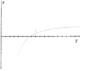
Fig.

2.1

shows a plot of p vs T, in the limiting case

7

—>

00

. From the plot, maximum allowable sampling period is read approximately to be 0.69. This value is very close to the value To = 0.692 , which is the maximum T for $ /i(T )E in Lemma 3.5 to be stable.

Fig.

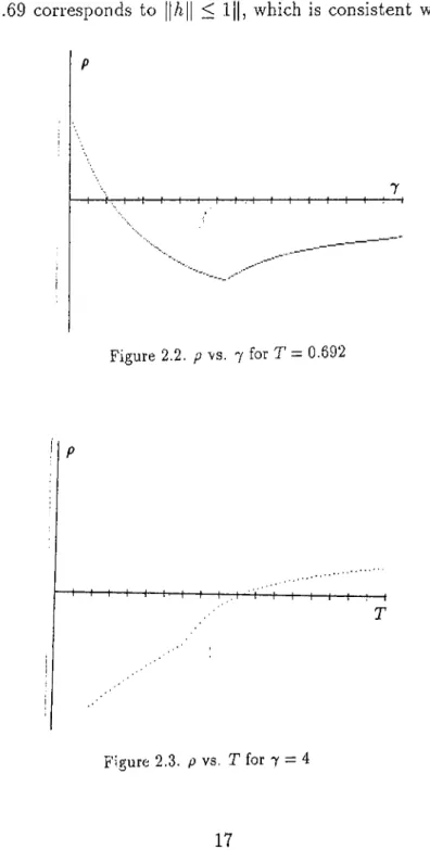
2.2

shows a plot of p vs

7

for T = To = 0.692 from which we observe that

7

values as small as

1.1

~

1.2

are sufficient to achieve robust stability. It is interesting to note that a value of

7

= 4 ~ 5 performs better (results in better stability degrees) than a very high value.

H--- 1— I----h -t-T-f—I--

1

---

1

---

1

---\---

1

---

1

---

1

---

1

---

1

--

1

Figure 2.1. pvs. T for 7 00

To check whether a controller corresponding to a fixed

70

and To also works for smaller T, we plot in Fig. 2.3 p vs T corresponding to

7

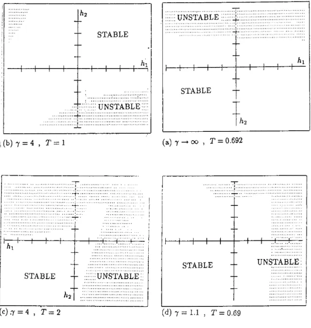
= 4. We observe that $ (T ) is stable for all 0 < T < 1.01, providing a positive answer to our question.

Finally we plot in Fig. 2.4, the stability regions in the space of the disturbance parameters hi and

/12

for different

7

and T values. We note that the largest circiilar region in the parameter space for

7

=

70

=

1.1

and

T = To = 0.69 corresponds to ||/i|| < 1||, which is consistent with the above analysis.

' P

-I---- 1. I ' I---- i---- 1---- 1---- 1---- h -H ---- 1---- 1---- 1---- 1---- 1---- 1---- 1---- 1

Figure 2.2. p vs. 7 for T — 0.692

— '— I— I— I— I— I— 1-7. 1 ' V— I— I— I— I— I— I— I

Figure 2.3. p vs. T for 7 — 4

/l

2

STABLE (b) T = 4 , T = 1 hj ■ UNSTABLE; -UNSTABLE ... A’ 1 1 1 1 1 1 h... !; 1 ; ... hi 1 1 -1____1---- i 1---1---1---1 1 STABLE 1 1 1 1 h-2 (a) 7 oo , T = 0.692 hi -i---^---H STABLE (c).7 = 4 , T = 2 ; u n s t a b l e: H— ^— \— h STABLE H----

1

UNSTABLE: (d) 7 = 1.1 , r = 0.69

Fig 2.4. Stability regions in the parameter space

Chapter 3

ROBUST DECENTRALIZED SAMPLED

DATA CONTROL OF

INTERCONNECTED SYST' I: \ IS

In this Chapter, we investigate using the results obtained in Chapter

2

, robust stabilization of interconnected systems by decentralized single-rate sampled-data state feedback.

3.1

Interconnected Systems and Decentral­

ized Control

We consider a large-scale system consisting of N interconnected subsystems described as

Si : Xi = AiXi -b biUi -b bihJjXj , i e Af

j'eA/·

(3.1)

where C 'RA' and

6

% are the state and the input of the subsystem and Af = {

1

, 2 , . . . , The constant matrices A,· G 7?."'^” ' and bi € 7?T' define the decoupled subsystems

S f : Xi = AiXi -b biUi , i £ Af

19

and hj- = [hi h'2 . . . h[^.] are constant bounded but unknown interconnection

parameters.

VVe assume that the decoupled subsystems are controllable and A{,

6

,- are in controllable canonical form as in (

3

.

2

)

Letting X = u = A = B = H = Xl X2 ,xjf [ui U

2

. . . Un]^ diag{A i, A2, . . . , An} d iag{

6

i, b2,..., b N } N,N (3.3)

the interconnected system in (3.1) can be described compactly as

<5 : i = (/1 + BH )x + Bu (3.4)

As can clearly be seen from the description in (3.4), the perturbation term B H due to the interconnection satisfies the matching conditions. Then generalizing the result of Chapter

2

to multi-input systems, we can assert that the system S can be stabilized by a sampled-data state feedback control. In the following we will show that this can be achieved by a much more restricted control, namely, by decentralized control.

Imitating the structure of the control law considered in Chapter 2, we choose the decentralized sampled-data state feedback control as

U i■ [t) = kf(t)xi{m T) , mT < t < [ m + 1)T , i Ç. jV

where ki{t) are T-periodic time-varying gains, that is,

ki{t + T) = ki{t) , i > 0 , i e A f .

(3.5)

(3.6)

Having the result of Chapter

2

, a natural choice for ki{t) would be

ki{t) = k j^ a ,{t) , 0 < ^ < T , i e j V (3.7)

where

and the matrices A;,· , i ^ M are to be determined. Letting

K

= diagfArJ^, k^,...,kjj]

K{t) = di&g{kj{t), kj{t),...,kjf{t)}

^K( t) = diag{$ifc,(i), ^2h( t ) , - - - , ^NkA^) }

we observe from (3.3) , (3.7) and (3.8) that

and (3.8) (3.9) (3.10) (3.11)

K(t) = Ki K{ t ) , 0 < ( < r

Thus rewriting (3.5) using (3.11) in a compact form as

u(:t) = K§ K{ t - m T)x{m T) , mT < t < {m -\-l)T (3.12) interconnected closed-loop sampled-data system becomes

S : x(t) — {A + + B K ^ K { t — mT)x(mT) , mT < t < (m.+1)T.

(3.13) Noting that (3.13) is just a multi-input version of (2.15), it follows from Lemma

2.1

that the solution of S is given by

x(t) = Ф(А — т Т)х{т Т ) , тТ < t < { m + l ) T (3.14) where ф(^) = Фк{г) + Г Фя(А -

5

)БЯФл-(з)Ьб (3.15) Jo ' with Фя(·) as in (3.10) and Фя(А) = . (3.16)

Following the same argument as in Section 2.1, we observe that the closed-loop interconnected sampled-data s

5

'^stem S of (3.13) is stable if the

accompanying discrete time system T> of (

2

.

22

) is stable, where Ф(^) is now obtained from (3.15) as

Ф (Г) = Ф / г ( Т ) + Г ^h{T - s)BH^K{s)ds (3.17) Jo

Although Ф(Т) of (3.17) is almost the same as that of (2.23), extension of Lemma 2.3 to multivariable case is far from being trivial. The main difficulty in obtaining an alternate expression for Ф(Т') as in (2.28) lies in the definition of the matrices E and E in (2.29). In the next section we propose an expansion procedure to overcome this difficulty.

3.2

Expansion of The System

Let n be an arbitrary integer satisfying n > Uj , i G J\f. Consider the following subsystems

. ¿i — A-jX,' “b “I” ^ ) h^h‘j00j , z G A7

ieM

associated with the subsystems <S, of (3.1), where x,· € 77." and

Ai Ei

0 Ai

,

0

bi

, Щ = 10/‘ и

(3.18) (3.19)

with Ai G ("·-” ·) and Ei G being arbitrary matrices, and

6

,·, hij G 77." are obtained by padding

6

,· and hij with zeros. Using the compact notation of (3.4), the overall interconnected system consisting of the subsystems of Si of (3.18) can be described as

S : X = (/1 + B H )x + Bu (3.20)

where the matrices A , B ^ H and the vectors x and u are defined as in (3.3).

Associated with the control law in (3.12), we apply the sampled-data control

£((t) = K ^k{^ ~ rnT)x{mT) , mT < i < (m +

1

)T (3.21)

to S to obtain

5 :

$m = (A + BH)x{t) + BK^K{t-rnT)xirnT)

,

m T < t < { m + l)T

(

3

.

22

)

where K and (¿) are defined as in (3.9) and (3.10) with

k j =

[0

¿T]. (3.23)

We recall [10] that the syslc!;^ ' of (

3

.

21

) is called an expansioii ' ! die system <5 of (3.13) if there e.xist : i matrix V withiull row rank such i h.. i '.lie relation

x(i) 1/5(0 , i > 0 (3.21)

holds between their solution:. ■,vh never a;(0) = y 5 (0 ). We now prove the following.

L em m a 3.1 T/ie system

6

(3.13)

' /) is an expansion o f the system S of

P r o o f: Let the matri<

and let

" /..,J ,

)e defined as

i e M (3.25)

V = diag{ Vi Vn} (3.26)

Then obviously V is o f full row rank. By construction oi A , B , K and H

we have ^ , VA = A V , V B - - B , k ^ K V , H = H V (3.27) so that Hence f / ( i + M ) = {A + B K )V V {A + B H ) = {A + B H )V V^K {t) = ^K {t)V 23 (3.28) (3.29)

which, together with (3.15), imply that

where $ //( i ) is defined as in (3.17). The proof then follows from (3.14). Note that by the construction of V in (3.25) and (3.26) we have

i ' i ' · / (3.31)

and

(3.30)

$ ( / ; (3.32)

The importance of Lemma 3.1 is that using the expansion of the system we can find an alternate expression for $ (i) as in Section 2.2. Our gain in dealing with <S rather than S is that the subsystems of S are of the same dimension n which makes a generalization of Lemma 2.3 possible.

Due to the relation (3.24) stability of S implies the stability of

6

, but the converse is not generally true. We may have S unstable but S stable. Since we are interested in the stability of S only, we use the expansion just for obtaining an alternate expression for $ (t).

3.3

structure of ^(¿)

The aim of this section is to provide the decentralized version of the alternate expression for $ (t) as in Lemma 3.2, which will enable us to investigate the stability properties of S. For this purpose we first specify the matrices A, and Bi of in (3.19) as ' 0 1 . , 0 0 .. 0 ■ 0 ■ 0 0 . 0 0 . . . o ' .. 0 0 0 . , 0 0 . , .. 1 • 0 . 0 0 . , 1 0 ., ,. 0 .. 0 __{(n —n,· )X ni} (3.33) 24

For this specific expansion ot the system, we observe that (A,·, ¿¿) is in canonical controllable form, similar to (A,·,

6

,·).

We define the following matrices lor the expanded system in parallel to (2.24). Ui = Gii = 0 0 0 1 0

. . .

0 0 . . . 1 0

0

...

0

0

. . .

0

_ r< . _ , U r , , — 0 I ... 0 1 0 0 . . . 0 0 /4' - 0 0 0 ■ 0 0 C i j = 0 ad L 0 ad Cj 0 . . cb_{'-'n .J} 5 — . 4 ·’ C2 • · ¿ij J C = {C{j)N,N ) ,G — {Gij)N^N

1

U — diag{Ui} wiith se - .^1 ~ _{h f else} (3.34) (3.35) We then state the following identities which are the natural decentralized extension of Lemma 2.2.

L e m m a 3.2 The matrices in (3.34) satisfy the following identities.

a) GU = UG , CU = UC b) GC = CG c) UB = 0 , UC =--0 , UA - rr'^ d) G ( I - U U ^ ) = G , {I - I ' - '

e) A + BH = C + U^

25 :7 [:’''(^]r = C

P r o o f: All these identities follow from the definitions and from

n

—1

n

-1

G i ,- = T ,h U U [ . Ca = Y :r > J ’\ ■

/=0

.

We omit the details here. Finally, letting

G = G U = UG , C - CU = UC

we prove the following fact for the expanded system S.

L e m m a 3.3 $ (i) in (3.30) can be expressed as

$ (i) = f ^H(t - 5)S#A-(s)di JO where t

=0

(3.36) (3.37) (3.38) (3.39) 1 = 0

P r o o f The proof follows exactly the same lines as the proof of Lemma 2.3, and is therefore omitted

Using the alternate expression in (3.37) for $ (t) and (3.30), we can rewrite $ (T ) as $ (T ) = U $ (T )U ^ rj^ ^ K { T ) - ' ^ H { T ) t ^ m K { T ) + [ ^h{T - s)J:^K{s)ds Jo = V (3.40) Similar to (2.38) we decompose (3.40) as $ (T ) = - y l > ; / ( r ) S y ^

4

- R(T) , where R(T) = V(InN + + y T / i n i T - (s)di Jo (3.41) (3.42)

which we will use for analyzing the stability of S in the next section.

3.4

Stability Analysis

In this section, similar to the case of single input systems, we will show that stability of $ (T ) depends crucially oix V ^h{T)TjV'^^ which is itself independent of the local feedback gains. For doing this we will show that the norm of R{T) in (3.41) can be made arbitrarily small by choosing high-gain local feedback controllers.

Imitating Lemma 2.4 we state the following.

L e m m a 3.4 Let the local feedback gains ki = ^¿(

7

) be chosen such that the eigenvalues o f Ai -|- hikj are placed at

7

//I, where g] are arbitrarily fixed, distinct negative real numbers, and

7

is a positive gain parameter. Then, for any Bh >

0

, a7iy T > 0, and any e > 0, there exists a

70

> 0 such that

for all

7

>

7

o, where

||iJ(T)|| < e

denotes the spectral norm.

(3.43)

P r o o f: From (3.23) and (3.30) we hawe

0

<hifc

.(0

where for any fixed T > 0

lim ||$,-,.(T)|| =

0

, i e A ^

7—

^00

(3.44)

(3.45) as has already been shown in the proof of Lemma 4. On the other hand, letting Ii{T) = [ ' e^'(^-‘ )L;-$.-^,(5)ds (3.46) Jo substituting = r,M ,e‘ >‘T r M g (3.47) 27

where Mi , F,· and Di are siniilar to M , F and D defined in (2.41) - (2.43), and using the identity i?iF,· = i?,·, we have

1|/.(T)|| < \\EiMi\\\\Mr^r-^\\\\ r . (3.48)

J

0

Since for a fixed T > 0 , is bounded for all

3

G [0 , T], it follows from (3.50) that

T

\\IiiT)\\ < Bii (3.49)

for some finite Bu, where fn = m a x {/ij}. Therefore, for every T > 0 and

a,ny \\H\\<Bh ^

l i m l l / e^"'(^-^)T;.$a-.(5)ds||=0 . (3.50) 7-^00 Jo

Then (3.25), (3.44) and (3.50) imply that

lim $ifc,(r)K·^ = lim

7—

^00

7—>-oo = 0 ,

i e M . (3.51)

Hence, for all H satisfying j|if|| < Bh and for all T > 0, we have

lim V {I + S)$/i(T)H"'^ —

0

7—i-OO

To bound the integral term in (3.42), we first note that

^A'(-s)F'·'^ = diag

(3.52)

Ii{s)

Dikiis) (3.53)

where /.(s ) is defined in (3.46). Using the expression for E given in (3.39), we have E 4 K ( i) r ^ = E C 'f f d i a e

= EC 'G diag

j=o

if rM

I [

J

0

(3.54) 28

where the second equality follows from the definition oi G — {Gij)N,N in (3.35). Therefore

V ê n i T - =-- v j ^ ^h{T - s)Sdiag

0

so that by (3.49) and boundedness of ^h{T — s) on [OjT], we have lim V

7-^00

l^ds (3.55) / / ^h(T - s)E $ft-(s)dsV ’^ = 0 (3.56) %/

0

for all r > 0 and all H with |(if|| < Bh. This completes the proof.

Lemma 3.5

For a given Bh > 0 there corresponds oTq > 0 such that for all

0

< r < To and all |¡//[| <

Bh.,

is stable in the discrete sense.

Proof

Since every block entry of C and G are triangular matrices with zero diagonal, S has the same structure, that is, each block E¿j of É = is a triangular matrix with zero diagonal. This implies that all eigenvalues of the matrix F $ //-(

0

)E F ^ = VtlV^ = are at the origin.

The rest of the proof is the same as the proof of Lemma 2.5.

Now we can state a decentralized version of Theorem 2.1, which, is the main result of this chapter.

Theorem 3.1

For every

Bh

0

there exists a

T

q

> 0

such that for any 0 < T < To there exists a decentralized sampled-data state feedback controller o f the form (f!.12), which stabilizes S for all ||if|| < Bh·

Proof:

Having Lemmas 3.4 and 3.5 in place of Lemmas 2.4 and 2.5 respectively, proof of this theorem is exactly the same as the proof of Theorem

2.1.

Similar to the centralized case. Theorem 3.1 provides a constructive procedure to determine the saro.piing period and the local controllers in terms of the bound of the perturbations, but not of the perturbations themselves.

Chapter 4

MULTIRATE ROBUST

SAMPLED-DATA CONTROL

In this chapter we vr-n'·· t.he results of Chapter 3 to the case where local controllers use valu'·; 'ji i,UiLes sampled at different rates.

4.1

Multirate Decentralized Control

Consider the interconnected system described by (3.1), or in equivalent compact notation by (3.4), which we repeat below for easy reference

Si ¿i(t) = AiXi{t)

+

biUi{t)

+ ^

bihJjXj . S x{t) = iA + BH)x{t) + Bu(t) .

(4.1) ( .4 - :

We choose the multirate decentralized control law as

Ui{t) = kf {L)xi{mTi) , niTi < i < (rn + l)Ti , i G Af (4.3) where

Ti = MiT , i e Ai (4.4)

is the sampling period of the i*^ subsystem, with Mi being a positive integer. The time-varying gain ki(t) in (4.3) is periodic with period Ti, and is chosen as kj (t) = kj^ik,{t) , o < t < T i , i e M where is defined in (3.8). Let and M = l.c.m(Mi) , T = M r . (4.5) (4.6) (4.7)

We define r as the basic time unit, and T as the common sampling period. Note that each Ti is a an integer multiple of r , and T is an integer multiple of every T,·.

To describe the evolution of the state of the closed loop system consisting of <S in (3.17) and the feedback law in (4.3), consider an initial time instant

t o = ^ m T + h , / =

0

,

1

, . . . M - 1 ; m = 0 , 1 , 2 , . . . . Then for each i e Af,

there exists unique integers 0 < mi < {MfMi — 1) and

0

< r,· < M,· — 1 such that

It = m,T,· -}- r,r , i e Af . . (4-8) By (4.3), (4.5) and Ti periodicity of ki{t) in the interval to < t < t o + t , the input to the subsystem is given by

Ui{t) = kj^ik,{t - m T - miTi)xi{mT + miTi) . (4.9) Substituting (4.9) into (4.1), we obtain

<5 : x{t) = {A + BH) x{ t) + BikJ^^kiit - m T - m,Ti)xi{mT + miT) ,

I'eA/·

m T + /r < i < m T -f ( /-b l ) r , (4.10) where Bi are the columns of B in (3.3). The solution of (4.10) at t = io + r =

mT -t- (/ -b l ) r is obtained as

x [ w T + ( / + l )r] = ^H ir)x{m T + lT) (4-H)

+ Y ] [ 4>h(t - 5)i7iA:)^$,7;, (5 + nT")d-5 X i { m T m i T i ) .

Ji = diag{0, (4.12) and noting that

DK^ K{ h) Ji x { h) , i i , t 2 > 0 (4.13) where is defined in (3.10), (4.11) can be written as

x[mT -\- (/ + l)r ] = $//(r)a:(m T ' + ^t) + ^ I[riT)Jix{mT + rtiiTi) (4.14)

ieJ^

where ^

/ ( A j - / i > j i ( r - 5 ) .e /i i $ /i ( 3 + A)d5 , A

> 0

. (4.15)

0

To put (4.14) in a more convenient form, let us define for each 0 < I < M ~

1

, the index set

M l = { i ^ M : It = rriiTi for some integer m,·} . (4-10)

In other words. A i s the index set of those subsystems whose samplers are closed at time ruT f It. From (4.8), it follows that for i ^ M i , r,· =

0

, that is rriiTi = It. we now rewrite (4.14) as

x[mT + (/ -f l)r ] = [$ ir(r) + I(0)Ji]x{mT + m ,r,·)

ieJ^i

+y))/(r,-r) J,a:(m2' + ruiTi), / = 0, 1, . . . , M - 1,(4.17)

¿

6

^v-A/i

Using (4.17) recursively for / = 0 , 1 , . . . , M —

1

, we obtain

V : x[{m + 1)T] = ^{ T) x{ mT) , (4.18) where

$ (T ) = $ M - i ( r ) - - - $ i ( r ) 4 : \ i ' ( T ) , (4.19)

H r ) = $ i /( r ) + 7 (0 )J.· , / =

0

,

1

, . . . , M

- 1

i&Ml

and lP(r) is a sum of product terms each of which contains at least one 7 (rr) term with

1

< r < max(Mi) —

1

.

(4.18) represents a shift-invariant discrete-time system V, which describes the transitions of the closed-loop sampled-data system over the common sampling period T. In the next section we investigate the stability properties of X).

Defining

4.2

Stability Analysis

The decomposition in (4.19) is the key to stability analysis of $ (T ). We start with an investigation of the / ( r r ) terms in li’ (r).

L em m a

4.1

Let ki = ki(j) be chosen as in Lemma 3.4· Then, for every fixed

r >

0

and e >

0

there exists a

70

such that for every

7

>

70

, ^ for all t > T.

P r o o f: From (2.24),

kf^ik,(t) = kjTiMie^‘ ^Mr^Tf^ . Noting that

l|ifr,|| < K n "· ,

for some finite Aii,·, wliich is independent of

7

, we have

where fii = m a x {/ii) and the proof follows.

(4.20)

(4.21)

(4.22)

L em m a

4.2

Let k, = A;,(

7

) he chosen as in Lemma S.f· Then, for all r > 0

, Bh > 0 and e > 0 there exists a

70

>

0

such that

||/(rr)|| < e

for all r > 1, for all

7

>

70

and for all LI with ||if|| < Bh ■

(4.23)

P r o o f: From (4.15)

i|/(rr)|| r||$„(T-s)||||5||||/f$,.·(»+»-

t

)||<1

s

,

(4.24)

Jo

the proof follows from Lemma 4.1 , and the boundedness of ~ -s) for

5

e ( 0,r).

An immediate consequence of Lemma 4.2 is that

or equivalently,

7— »-OO for all r > 0 and all bounded H

lim ^ (t) =

0

7— »-CO M

-1

lim $ ( r ) = r r lim $ / ( r ) V— '' ' .A .-1. / -V— ' '

/=0

7 —>00 (4.25) (4.26)

Before proceeding any further, we would like to point out that $;(r)represents an approximation to the state transition matrix on the interval [mT + /r, m T + ( / + l ) r ] . This is reasonable, because under high-gain feedback the control applied to thoSe channels whose samplers are inactive at to — mT It are effectively zero, and only the channels indicated by

the index set Mi contain significant control signals. Note that in the case of identical sampling in all subsystems we have M = 1 , T = t, Mo = M s o

that ^'(t) = 0 and (4.19) reduces to

$ ( T ) = # o (r) = $ //( r ) + / (

0

) , which is the same as (3.17) as expected.

We now turn our attention to an investigation of the indix i· matrices in (4.20). Letting

S

i

.

i&ZJ'i we write J.,(t) = i i f ( r ) + / ( 0 ) 5 , = [4h(t) + 5(0)15, + $ „ ( r ) ( / - 5,) . Now using the expansion procedure in Chapter 3, we obtain

4 f f ( ’ ·) + 5(0) = - I /4 H (T )i :V '· '+ B (t) , (4.27) <i>/(r) (4.28) (4.29) (4.30) where V, and i?(r) are defined in (3.26), (3.39) ,(2.18) and (3.42). Substituting (4.30) into (4.29) and rearranging the terms we get

$ ,( r ) = [-V ^ H iT )tV " + R{T)]St + V ^ H { T ) V ^ { I - S i )

= V ^ n ( T ) { I - S , - t S , ) \ M + R{T)S, (4.31)

where Si has the same structure as Si except that its diagonal blocks have sizes n X n rather than n,· x n,·. From the analysis in Chapter 2, we know that

R {t) —

0

(4.32)

7—^00

for every fixed r > 0 and all H with j|//|| < Bh- Using this property, we write from (4.31)

lim $ ,(r ) = U$,(r)U '^ , 7— »-OO

where

Hence from (4.26), we have

r M - i ‘ lim # ( r ) = V 7— ►OO ^ ^ n M tKI - S i- SSi) ¡=0 (4.33) (4.34) (4.35) which has the following stability property.

L em m a 4.3 To every > 0 there corresponds a To >

0

> ihat the matrix in (4-35) is stable in discrete sense for all 0 < T < Tq an·: u- all H with II

//11

< Bh. P r o o f: Consider [lim $ ( r ) ] r . o = U 7 —>00 ^ M

-1

n(/-¿^/-s5/)

L 1=0 (4.36)

where each term / — Si — TSi in the product is a block matrix with lower triangular blocks. In particular, for / = 0 , So = I so that

I - S i - t S i = - t , (4.37)

wliose blocks have zero diagonals. This implies that the whole product in (4.36) has the same structure. The proof then follows the same lines as the proof of Lemma 3.5.

We are now ready to prove our main result on stabilizability of the system <S in (4.1).

T h e o r e m 4.1 For every Bh > 0 there exists a To > 0 such that for any

0

< r < To there exists a decentralized multirate sampled-data state feedback controller o f the form (4-3) which stabilizes S for all ||ii"|| < Bh ■

P r o o f: Fix To as in Lemma 4.3, so that limy_.co ^{T ) in (4.35) is stable for all

0

< T < To and for all H with ||Lf || < Bh- Then choosing

7

sufficiently large so that ^ ( r ) in (4.19) and R{t) in (4.31) are small enough not to destroy the stability of $ ( T ) , the proof follows.

Chapter 5

CONCLUSIONS

In this thesis we considered robust sampled data stabilizabilit}'· of

• single-input, linear, time-invariant systems under perturbations that satisfy matching conditions, using state feedback;

• interconnected systems composed of smaller subsystems with uncertain interconnections that satisfy the matching conditions, using decentral­ ized state feedback; and

• interconnected systems using decentralized multirate sampling.

We have shown that robust stabilization can be achieved in all three cases for all sampling periods smaller than a critical value Tq.

The main result of Chapter

2

guarantees the existence of a stabilizing sampled-data controller for every fixed sampling period smaller than Tq.

Whether a controller designed for To works for all smaller sampling periods remains to be an open problem.

Another problem that is worth to investigate is to extend the results obtained in this thesis to more general perturbation structures. It is strongly believed that all perturbation structures which allow for robust stabilization

using continuous-time state feedback can also be handled by sampled-data state feedback.

Finally, design of decentralized controllers based on single or multirate sampled outputs rather than states is a closely related research topic.

Bibliography

[

1

] E. J. Davison “The decentralized stabilization and control of a class of unknown nonlinear time-warying systems.” Automática

10

p. 309 1974 [2] B. A. Francis and T. T. Georgiou“ Stability Theory for Linear

Time-Invariant Plants with Periodic Digital Controllers” /FF'E Trans.. Automat. Contr..,vo\ AC-33, pp.820-831 Sept. 1988.

[3] K. J. Ástróm, P. Hagander and J. Sternby “ Zeros of Sampled Data Systems,” Automática.^ vol. 20 no. l,pp. 31-38,1984

[4] I. Horowitz and 0 . Yaniv, “ Quantitative design for SISO nonminimum- phase unstable plants by the singular-G method,” Int. j. Contr.. vol. 46 no.

1

pp. 281-294, 1987

[5] P. T. Kabamba “ Control of Linear Systems Using Generalized Hold Functions” /F E E Trans. Automat. Contr.,vol AC-32, pp.772-783 Sept. 1987.

[

6

] B. D. 0 . Anderson and J. B. Moore “ Time-Varying Feedback Laws for Decentralized Control” IEEE Trans. Automat. Contr.,vol AC-26, pp. 1133-1138 Oct. 1981.

[7] P. P. Khargonekar, K. Poola and H. Tannenbaum “Robust Control of Linear Time-invariant Plants Using Periodic Compensation” IEEE

Trans. Automat. Contr.,vol AC-30, pp. 1088-1096 Now. 1985.

[

8

j M. E. Sezer and D. D. Siljak “ On Decentralized Stabilization and Structure of Linear Large scale Systems” Automática vol. 17 no. 4 pp. 641-644 1981

[9] M. E. Sezer and D. D. Siljak “ Robust Stability of Discrete Systems”

Int. j. Contr. vol. 48 no. 5 pp. 2055-2063, 1988

[10] Ikeda M. and D. D. Siljak (1980) “ Overlapping Decompositions, Expansions and Contractions of Dynamic Systems. ” Large scale systems,

1

. ,29, 38