Selçuk J. Appl. Math. Selçuk Journal of Vol. 7. No.2. pp. 91-101, 2006 Applied Mathematics
Wald-Type Statistics In Heteroscedastic Linear Models Esra Akdeniz1 and Michael G. Akritas2
1Gazi University, Faculty of Arts and Sciences, Department of Statistics, Ankara
Turkey;
e-mail: esraakdeniz@ gm ail.com
2Penn State University, Department of Statistics, USA
e-mail: acq@ psu.edu
Summary.In this paper we consider the heteroscedastic linear models and con-sider Wald-type test statistics for the hypothesis of no factor effects and no inter-actions. Designs with independent data are considered. The statistics based on the original observations appear to be new. They test the usual parametric null hypotheses and provide useful alternatives to the classical F-test especially in the presence of variance heterogeneity. The statistics based on ranks have been proposed in Akritas and Arnold (1994), Akritas, Arnold and Brunner (1997) and in Akritas and Brunner (1997) for the purpose of testing certain nonpara-metric hypotheses. Simulation programs in MATLAB are developed and the results are presented.
Key words:ANOVA (Analysis of Variance) design, Heteroscedasticity, Linear Models, Wald Statistic
1. Introduction
ANOVA, obviously relies on the assumption that variances are equal in all groups. With few groups and equal sample sizes, failure to meet this assumption simply costs power however with unequal sample sizes, this can inflate the Type I error rate. The more groups there are, the worse this is, see Bryne (2005). As it will be demonstrated in the paper, the Wald method gives a closed form test-statistic for any of the common hypotheses in any ANOVA design (unbalanced and/or heteroscedastic).
Two main methods for constructing test statistics are the likelihood ratio (LR) method and the Wald method. LR method is applied widely in linear models. For example, the usual F- statistics for testing hypotheses in ANOVA designs
are LR statistics assuming the normal distribution. However, the LR F-statistics do not always have a closed form expression especially in unbalanced situations. For example there is no closed form expression of the F statistic for testing no interaction effects in the unbalanced two-way ANOVA( see, Arnold 1981). Moreover adaptations of the LR-F statistics in heteroscedastic ANOVA designs have not been considered in detail, especially when the variances are unknown. For a general discussion about assuming known variances see Arnold (1981), Ch 13. Under the assumption of equal variances, the pooled- variance t-test is the likelihood ratio test (Hogg, Mc Kean and Craig (2005),p.439) but the common two-sample test-statistic assuming different population variances is not a LR statistic.
The common test-statistic in the heteroscedastic two-sample problem can be ob-tained as a LR statistic assuming, to begin with, that the variances are known and then substituting estimates for the variances. This is in the spirit of Gong and Samaniego (1981) who studied maximum likelihood estimation for a pa-rameter using consistent estimation of a nuisance papa-rameter . However, it is much simpler to think of the heteroscedastic two-sample test-statistic as a Wald-type statistic. Wald’s method constructs test statistics using estimates of the parameters of interest and estimates of the corresponding covariance matrix. Thus, if , is a possibly vector valued parameter of interest, ˆ, a point estimate,
ˆ
ˆ, an estimate of the covariance matrix of ˆ, and 0, the value of specified by the null hypothesis, Wald’s test statistic is
(1) (ˆ − 0)0ˆˆ−1(ˆ − 0)
The estimator ˆ can be maximum likelihood, moment, or any type of estima-tor. In this sense Wald’s method is more general than the LR method which requires the specification of an underlying distribution. As with LR test statis-tics, the exact distribution of the Wald statistic in Eq.(1) is, in general, unknown but by the standard asymptotic theory it is approximated by a 2distribution with degrees of freedom equal to the rank of ˆˆ. We note that the asymptotic 2distribution of the Wald statistic requires only that ˆ is asymptotically normal which is true for a wide class of estimators, regardless of parent distributions of the original observations.
This paper focuses on the application of Wald’s method for constructing alter-native hypotheses in, possibly heteroscedastic, ANOVA designs. The basic idea is that any of the common hypotheses, in any design, can be expressed as a set of contrasts being equal to zero. When viewed as such, the Wald method applies naturally with being the vector of contrasts, 0= 0 and by estimating the covariance matrix of ˆ.
This paper is organized as follows. The derivation of Wald statistics for two-factor ANOVA are given in section 2.1,also it is mentioned that the hypotheses
in any ANOVA design can be written as a set of contrasts of the elements of the vector of cell means. The uniqueness property and asymptotic distribution of Wald statistics are given in sections 2.2 and 2.3 subsequently without proofs. Simulation study is conducted in section 3 and several statistics are compared based on their Type I error and Power values.
Throughout the article we use the following notation. 1 denotes the × 1 column vector of 1’s, and = 1 × 10. The -dimensional identity matrix is (diag{1,. . . .,1}) is denoted by , and = (1−1| − −1). The weight matrices are denoted by = (2 )0, ∗ = (1 ), = (1 )0,∗= (1 )Replacing an index by · denotes averaging over all values of that index.
2. Test Statistics Based On Contrast Estimates For Independent Data In the first subsection of this section, we will first derive the general form of the Wald statistic for the hypotheses of main effects and interactions in any ANOVA design. To eliminate dependence on a particular distribution, the main and interaction effects will be estimated by the method of moments using the group sample means to estimate the group population means. It will be seen that the general statistic for any hypothesis in any crossed classified design will be of the form
(2) = ( ˆ)0( ˆ 0−1 ˆ
for some contrast matrix C. In the second subsection, we will present a result regarding the uniqueness of the Wald statistic, and in the final subsection we will mention about its asymptotic distribution. (The proofs are available upon request.)vRemark 2.1 The method of moments gives the same estimators as the method of maximum likelihood applied to the full model (i.e. all effects are there) under the normality assumption. Unlike Wald’s methods, however, the usual F-statistics are normal-based likelihood ratio statistics requiring the evaluation of MLE under the null hypothesis. In unbalanced situations, this MLE does not have a closed form expression. This is the reason why, except for one-way ANOVA, the F-statistics displayed in textbooks correspond to the balanced case.
2.1 Derivation of Wald Statistics in ANOVA designs
We will illustrate the construction in a two-factor ANOVA design. Let the observation that corresponds to row level i and column level j be denoted by , = 1 = 1 = 1 The set of means can be decomposed as
= + + +
X =1 = 0 X =1 = 0 X =1 = X =1 = 0 ∀
where > 0 ∀ > 0 ∀and P = P = 1. Under these set of constraints, = ¯·· = ¯·− = ¯·− = − − − where ¯ ··= X =1 X =1 ¯·= X =1 ¯·= X =1 The moment estimators of are
ˆ = ˆ¯·− ˆ ˆ= ˆ¯·− ˆ ˆ = ˆ− ˆ − ˆ− ˆ where ˆ = ¯·= 1 X =1 =ˆ X =1 X =1 ¯· ˆ ¯ ·= X =1 ¯· ˆ¯·= X =1 ¯·
Remark 2.2 Setting = − , we can always write = + + + + , which looks like the usual ANOVA model. However it differs from it in that the are not required to be normal, are not required to have the same variance as i,j change, are not required to have the same distribution as i,j change, and need not even have a continuous distribution.
For these reasons, the Wald statistics that are developed here apply to all types of ordinal (continuous and discrete) data. The common hypotheses tested in the two-way layout problem are
(3) 0() : = ¯·− = 0 ∀
(4) 0() : = ¯·− = 0 ∀
(5) 0() : = − ¯·− ¯·+ = 0 ∀
Any of the hypotheses in Eq.(3-5) can be written as a set of contrasts of the abx1 column vector = (11 1 1 )0.
Proposition 2.1 Any hypothesis, in any ANOVA design, can be written as a set of contrasts of the elements of the vector of cell means.
In the case of a two-way design, the contrast matrices for the hypotheses in Eq.(3-5) can be expressed through the elementary matrices introduced at the end of Introduction as follows:
= 0⊗ 10∗ = 10∗⊗ 0 = 0⊗ 0 Thus the hypotheses in in Eq.(3-5) are equivalently written as
0() : = 0 0() : = 0 0() : = 0
Let now C is the contrast matrix and consider testing the hypothesis. 0() : = 0. It follows that the Wald statistic for testing 0()is Eq. 2. Any of the common hypotheses in three or higher way layouts can be written as in 0() for some contrast matrix. Thus Eq.2 is the form of Wald statistic for any of the common hypotheses in ANOVA models.
2.2 The Uniqueness of Wald Statistics
The issue of uniqueness arises because the contrast matrix describing a partic-ular hypothesis is not unique.
Theorem 2.1 The Wald statistic does not depend on the particular contrast matrix.
2.3 Asymptotic Distribution of the Wald Statistic
Theorem 2.2 The asymptotic distribution of the Wald statistic is a chi square distribution with degrees of freedom equal to the rank of the contrast matrix. 3. Simulation Study
Throughout the paper we presented the Wald-type statistic as an alternative test statistic in case of heteroscedasticity. In this section we will illustrate some simulations including balanced, unbalanced, heteroscedastic and homoscedastic cases under normal distribution assumption. This section encompasses the sim-ulation studies for several testing procedures including the Wald-type statistic we presented, for comparing the Type I error and power based on 1000 samples. Simulation studies are based on generating three independent samples from nor-mal distribution for balanced, unbalanced, homoscedastic and heteroscedastic case and comparing achieved Type I error and power values. In some simula-tions all cell frequencies are assumed to be all equal to n, in others unbalanced designs are considered where cell frequencies are assumed to be different. Let a be the number of groups to be compared then the test statistics to be compared are the following:
Usual F statistic: This is the usual F statistic based on the assumption of homoscedasticity. = P =1 (¯− ¯··)2( − ) P =1
(− ¯)2( − 1)where a is the number of groups to be compared and N is the total size.
Heteroscedastic F statistic: = P =1 ³ ¯ ·−˜ ´2
( − 1)where a is the number of groups to be compared and ˜ ··= P =1 P =1 2 P =1 2
B-F 74 statistic: This statistic is based on Brown and Forsythe(1974) which assumes normality but does not assume homoscedasticity. The F statistic in that article is = P =1 (¯− ¯··) P =1(1 − ) 2
. The distribution of that F statistic may be approximated by that of Snedecor F statistic with a-1 and f degrees of freedom where f is implicitly defined by Sattertwaite approximate degrees of freedom formula 1 = P =1 2 − 1 where = (1 − )2 P =1(1 − )2. Original Wald-Type statistic: This is the Wald-type statistic presented in section 2.
3.1. Simulation Results
3.1.1 Balanced case and Normal Distribution
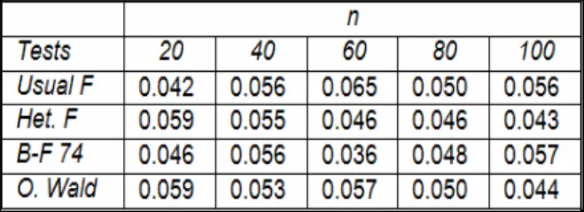
Table 1. Simulated Type I error for normal samples, homoscedastic and balanced case ,
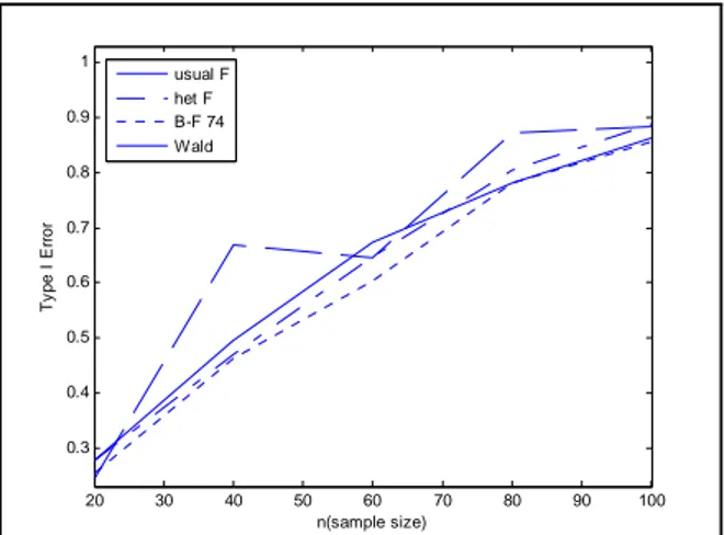
20 30 40 50 60 70 80 90 100 0.3 0.4 0.5 0.6 0.7 0.8 0.9 1 n(sample size) T y p e I E rr o r usual F het F B-F 74 Wald
Fig. 1 Sketch of Type I error vs sample size, homoscedastic case
Table 2. Simulated Type I error for normal samples, heteroscedastic and balanced case , 1= 2= 3= 0,1= 1 2= 9 3= 16,(1 − ) = 095. 20 30 40 50 60 70 80 90 100 0.04 0.045 0.05 0.055 0.06 0.065 0.07 0.075 0.08 n(sample size) T y pe I er ro r usual F het F B-F 74 Wald
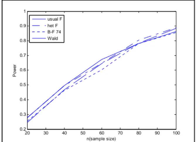
Table 3. Simulated Power for normal samples, homoscedastic and balanced case , 1= 1 2= 12 3= 148,1= 2= 3= 1,(1 − ) = 095 20 30 40 50 60 70 80 90 100 0.2 0.3 0.4 0.5 0.6 0.7 0.8 0.9 1 n(sample size) Po w e r usual F het F B-F 74 Wald
Fig.3 Sketch of Power vs sample size, homoscedastic case
Table 4. Simulated Power for normal samples, heteroscedastic and balanced case ,
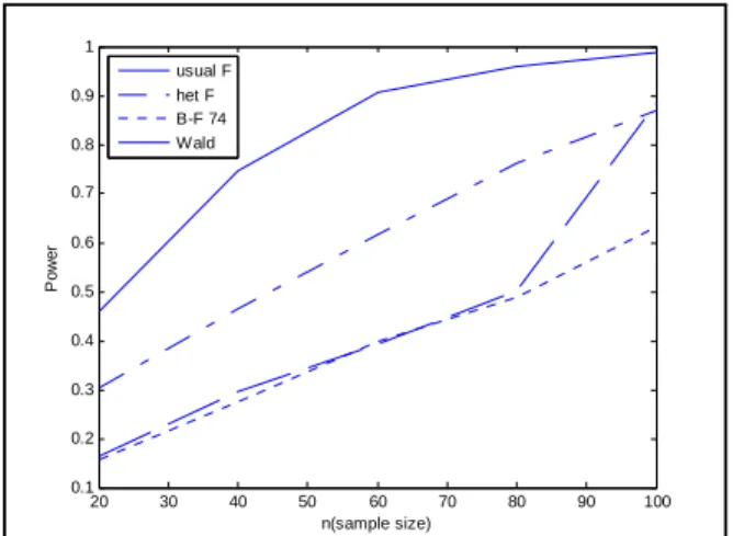
20 30 40 50 60 70 80 90 100 0.1 0.2 0.3 0.4 0.5 0.6 0.7 0.8 0.9 1 n(sample size) Po w e r usual F het F B-F 74 Wald
Fig.4 Sketch of Power vs sample size, heteroscedastic case
3.1.2 Unbalanced case and Normal Distribution
Table 5. Simulated Type I error for normal samples, heteroscedastic and unbalanced case,
1= 1 2= 1 3= 1,1= 1 2= 9 3= 16,(1 − ) = 095.
Table 6. Simulated Power for normal samples, homoscedastic and unbalanced case,
4. Results And Discussion
From the simulation results for the balanced and homoscedastic case under the normal distribution assumption all the statistics seem to work well (Table 1, Fig. 1). For the case of heteroscedasticity (Table 2, Fig. 2) the usual F statistic overestimates the alpha level.
The Wald-type statistic gives close values to =0.05. The heteroscedastic F statistic can also be considered to give an approximate result. The power values for the homoscedastic case are given in Table 3. For the homoscedastic case all the statistics seem to work well and all power values follow a similar pattern and approximate to 1 as the sample size gets larger(Table 3, Fig. 3). The power values for the heteroscedastic case are given in Table 4. It is very obvious that Wald-type statistic has the highest power and the heteroscedastic F statistic has the next highest power. The usual F statistic and the B-F 74 statistic have less power compared to the other two statistics as expected (Fig. 4). For unbalanced and heteroscedastic case the usual F statistic underestimates the alpha level (Table 5). It gives values around 0.02 which is very low compared to 0.05 however all other three statistics seem to work well. For heteroscedastic and unbalanced case (Table 6) the Wald-type statistic and the heteroscedastic F statistic have higher power than other statistics which again shows that both statistics work well under unbalanced and heteroscedastic cases.
5. Conclusion
From a theoretical point of view, Wald-statistic has many advantages when com-pared to the usual F statistic generally used in the literature. In this paper, we presented a construction method for two-factor ANOVA design but the method can be expanded to construct test statistics for other models as well. The con-structed statistics here are widely applicable and can be more preferable to other statistics in many situations due to the nice properties of Wald-statistics such as having a closed form, uniqueness and known asymptotic distribution. From the simulation results, generally speaking, for one way layout problem the Wald-type statistic and the heteroscedastic F statistic work well for the heteroscedastic cases. The Wald-type statistic is superior to the heteroscedastic F statistic in the case that it has a closed form, even for higher way layout. The derivation of the heteroscedastic F statistic for a higher way layout especially for unbalanced case is very difficult.
Finally, we conclude that further theoretical and simulation studies should be accomplished to obtain a better view of the behavior of these approximations.
Acknowledgement
Thanks to my thesis advisor Professor Michael Akritas for his guidance and support.
Nomenclature ⊗ kronecker product
References
1. M. Bryne, Physchology 502 Lecture Notes,
http://chil.rice.edu/byrne/psyc502/notes/2005_10_06_anova1.pdf, (2005) 2. M.G. Akritas, S.F. Arnold, Fully Nonparametric Hypothesis for Factorial Designs I: Multivariate Repeated Measures Designs, Journal of Am. Stat. Assoc. 89, 336-343 (1994).
3. M.G. Akritas , E. Brunner, A Unified Approach to Rank Tests for Mixed Models, Journal of Statistical Planning and Inference, 61, 249-277 (1997).
4. M.G. Akritas, S.F. Arnold, E. Brunner, Nonparametric Hypotheses and Rank Tests for Unbalanced Factorial Designs, Journal of Am. Stat. Assoc. 92, 258-265 (1997). 5. S.F.Arnold, The Theory of Linear Models and Multivariate Analysis, New York: Wiley (1981).
6. M.B. Brown, A. Forsythe, The Anova and Multiple Comparisons for Data with Heterogeneous Variances
Biometrics, 30, 719-724 (1974).
7. G. B. Gong, F.J. Samaniego, Pseudo Maximum Likelihood Estimation: Theory and Applications, The Annals of Statistics, 9, 861-869 (1981).
8. R.V. Hogg, J.W. McKean, A.T. Craig, Introduction to Mathematical Statistics, Prentice Hall (2005).