An analysis of pure robotic cycles

AN ANALYSIS OF PURE ROBOTIC CYCLES

a thesis

submitted to the department of industrial engineering

and the institute of engineering and science

of bilkent university

in partial fulfillment of the requirements

for the degree of

master of science

By

Serdar Yıldız

I certify that I have read this thesis and that in my opinion it is fully adequate, in scope and in quality, as a thesis for the degree of Master of Science.

Prof. Dr. M. Selim Akt¨urk (Advisor)

I certify that I have read this thesis and that in my opinion it is fully adequate, in scope and in quality, as a thesis for the degree of Master of Science.

Assoc. Prof. Dr. Oya Ekin Kara¸san

I certify that I have read this thesis and that in my opinion it is fully adequate, in scope and in quality, as a thesis for the degree of Master of Science.

Asst. Prof. Dr. Hakan G¨ultekin

Approved for the Institute of Engineering and Science:

Prof. Dr. Mehmet B. Baray Director of the Institute

ABSTRACT

AN ANALYSIS OF PURE ROBOTIC CYCLES

Serdar Yıldız

M.S. in Industrial Engineering Supervisor: Prof. Dr. M. Selim Akt¨urk

July, 2008

This thesis is focused on scheduling problems in robotic cells consisting of a number of CNC machines producing identical parts. We consider two different cell layouts which are in-line robotic cells and robot centered cells. The problem is to find the robot move sequence and processing times on machines minimizing the total manufacturing cost and cycle time simultaneously. The automation in manufacturing industry increased the flexibility, however it is not widely studied in the literature. The flexibility of machines enables us to process all the required operations for a part on the same machine. Furthermore, the processing times on CNC machines can be increased or decreased by changing the feed rate and cut-ting speed. Hence, we assume that a part is processed on one of the machines and the processing times are assumed to be controllable. The flexibility of machines results in a new class of cycles named pure cycles. We determined efficient pure cycles and corresponding processing times dominating the rest of pure cycles in the specified cycle time regions. In addition, for in-line robotic cells, the optimum number of machines is determined for given parameters.

Keywords: In-line robotic cell, CNC, scheduling, bicriteria optimization, control-lable processing times, robot centered cell, cycle time minimization, manufactur-ing cost minimization.

¨

OZET

TEK ATAMALI ROBOT˙IK D ¨

ONG ¨

ULER ¨

UZER˙INE B˙IR

ANAL˙IZ

Serdar Yıldız

End¨ustri M¨uhendisli˘gi, Y¨uksek Lisans Tez Y¨oneticisi: Prof. Dr. M. Selim Akt¨urk

Temmuz, 2008

Bu tezin konusu, aynı t¨ur par¸calar ¨ureten, belirli bir sayıda CNC makinadan olu¸san robotik h¨ucrelerde ortaya ¸cıkan ¸cizelgeleme problemleridir. Bu ¸calı¸smada, do˘grusal robotik h¨ucreler ve robot merkezli robotik h¨ucreler g¨oz ¨on¨unde bulun-durulmu¸stur. Bu problemdeki amacımız, birim ba¸sına d¨u¸sen ¨uretim maliyetini ve d¨ong¨u s¨uresini aynı anda enk¨u¸c¨ulten robot hareket d¨ong¨us¨un¨u ve bu d¨ong¨uye kar¸sılık gelen, makinalar ¨uzerindeki ¨uretim zamanlarını bulmaktır. Uretim¨ end¨ustrisindeki otomasyonlar h¨ucrelerin esnekli˘gini arttırdı. Ancak, robotik h¨ucrelerde esneklik ¨uzerine literat¨urde yeterince ara¸stırma bulunmamaktadır. Bir ¨ur¨un i¸cin gereken ¨uretim i¸slemlerinin t¨um¨u bir CNC makinada ger¸cekle¸stirilebilir. Ayrıca, CNC makinalardaki ¨uretim s¨ureleri, besleme ve i¸sleme hızına ba˘glı olarak azaltılıp arttırılabilir. Bu nedenle, bir par¸ca ¨uzerindeki ¨uretim i¸slemlerinin tek bir makinada yapıld˘gını ve ¨uretim s¨urelerinin kontrol edilebilir oldu˘gunu varsaydık. Esnek makinalar, yeni bir d¨ong¨u sınıfı olan tek atamalı d¨ong¨ulerin olu¸sturulmasına olanak vermi¸stir. Bu tezde tek atamalı d¨ong¨uler g¨oz ¨on¨unde bulundurulmu¸stur. Belirtilen d¨ong¨u zamanı alanlarında, di˘ger b¨ut¨un tek ata-malı d¨ong¨uleri ba¸satlayan tek ataata-malı d¨ong¨uler ve ¨uretim zamanlarını belirledik. Ayrıca, do˘grusal robotik h¨ucreler i¸cin, verilen de˘gerlere g¨ore en iyi makina sayısını belirledik.

Anahtar s¨ozc¨ukler : Do˘grusal robotik h¨ucre, CNC, robotik h¨ucre ¸cizelgelemesi, iki kriterli eniyileme, kontrol edilebilir ¨uretim zamanları, d¨ong¨u zamanı enk¨u¸c¨ultme, ¨uretim maliyeti enk¨u¸c¨ultme.

Acknowledgement

I would like to express my gratitude to my supervisors Prof. Dr. M. Selim Akt¨urk and Assoc. Prof. Dr. Oya Ekin Kara¸san for their instructive comments, guidance and encouragement in the supervision of the thesis.

I am also grateful to Assist. Prof. Hakan G¨ultekin for excepting to read and review this thesis and for his invaluable suggestions.

Finally, I would like to express my special thanks and gratitude to T ¨UB˙ITAK for the scholarship provided throughout the thesis study.

Contents

1 Introduction 1

1.1 Motivation . . . 4

1.2 Organization of the Thesis . . . 4

2 Literature Review 6 2.1 Robotic Cell Scheduling . . . 9

2.1.1 Cyclic Scheduling . . . 9

2.1.2 Multiple Part-Types . . . 10

2.2 Bicriteria Optimization . . . 12

2.3 Controllable Processing Times . . . 13

2.4 Summary . . . 15

3 Assumptions and Definitions 16 3.1 Bicriteria Solution Procedure . . . 19

4 Bicriteria Scheduling in In-Line Robotic Cells 22

CONTENTS vii 4.1 Bicriteria Analysis of Cm 1 and C2m . . . 22 4.1.1 Problem Definition . . . 23 4.1.2 Solution Procedure . . . 24 4.1.3 Discussion . . . 45

4.2 Optimum Number of Machines . . . 45

4.2.1 Problem Definition and Solution Procedure . . . 45

4.2.2 Discussion . . . 49

5 Pure Cycles in Robot Centered Cells 50 5.1 Minimizing Cycle Time with Fixed Processing Times . . . 51 5.1.1 Problem Definition . . . 52 5.1.2 Solution Procedure . . . 53 5.1.3 3-Machine Analysis . . . 64 5.1.4 Discussion . . . 67 5.2 Bicriteria Analysis of Cm 2 and C3m . . . 68 5.2.1 Problem Definition . . . 68 5.2.2 Solution Procedure . . . 69

5.2.3 3-Machine Case with Controllable Processing Times . . . . 75

5.2.4 Discussion . . . 80

List of Figures

4.1 m-Machine In-Line Robotic Cell . . . 24 4.2 C4

1 and C24 pure cycles . . . 44

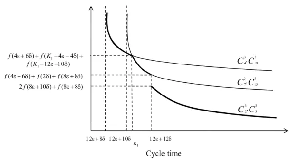
5.1 3-Machine Robot Centered Cell . . . 52 5.2 Cycle time-Processing time region where Cm

2 dominates the rest of

pure cycles . . . 62 5.3 3-machine cell analysis . . . 65 5.4 3-machine cell with controllable processing times analysis . . . 78

List of Tables

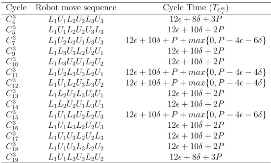
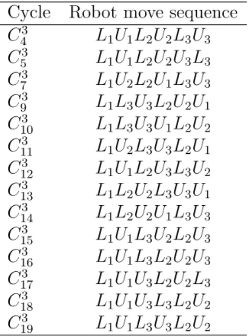
5.1 Some of the robot move sequences and corresponding cycle times in 3-machine robotic cells . . . 67 5.2 The feasible pure cycles in the cycle time region K < 12² + 12δ

and corresponding robot move sequences . . . 76 5.3 The processing times of optimum solutions of feasible pure cycles

in the cycle time region K < 12² + 12δ . . . . 77

Chapter 1

Introduction

The automation in manufacturing processes increased as the technology created special appliances for automation and improved the machines used in today’s in-dustry. Robots and Computer Numerically Controlled (CNC) machines are the important automation appliances that are considered in this thesis. Since robots increase the efficiency and reduce the labor cost, they are used in many diverse industries such as semiconductor manufacturing industry and electroplating ap-plications, chemical operations, and metal cutting industry [9]. In this thesis, we focus on the metal cutting applications in which the machines are predominantly CNC machines. The robots have different duties in different industries. One of the most important applications of robots is using them as material handling instruments. The robot handling costs may constitute from 10% to 80% of total costs according to the type of manufacturing facility [33]. A robotic cell is de-fined as a manufacturing cell composed of a number of machines and a material handling robot. We assume that there are no buffers at or between the machines, thus, at any time, a part is either on one of the machines, at the input or output buffers or on the robot.

In this thesis, we focused on the robot move sequence, the processing times on machines and the design of the robotic cell which are important decisions that have to be made in robotic cells. For the design of the cell, we consider two differ-ent layouts. The first cell layout considered is an m-machine in-line robotic cell

CHAPTER 1. INTRODUCTION 2

and the second cell layout is an m-machine robot centered cell. There is a single robot with a single gripper in both of these layouts. For the first cell layout, there is a bicriteria optimization problem of minimizing the cycle time and minimizing the manufacturing cost simultaneously. Additionally, as a design problem, the optimum number of machines in the cell is calculated. For the robot centered cell, the first problem considered is the minimization of cycle time that results in the maximization of throughput which is prominent in production planning. The second problem considered is the bicriteria optimization of minimizing cycle time and total manufacturing cost simultaneously.

Highly flexible CNC machines are used for metal cutting operations in robotic cells. The machines and the robot are used simultaneously in robotic cells. The cutting speed and the feed rate are controllable variables in CNC machines so that the processing times on these machines can be decreased at the expense of decreasing tool life and consequently increasing tooling cost. Considering fixed processing times is not convenient for real life problems in these robotic cells. For the bicriteria optimization problems considered in this thesis, the processing times on machines are assumed to be decision variables due to the controllability assumption.

As the flexibility of machines increase with the technological advance, new problems arise to be solved. The cyclic scheduling is widely studied in the lit-erature and we focus on cyclic schedules. In this thesis, we restrict ourselves to pure cycles resulting from the flexibility of machines. Pure cycles are defined by Gultekin et al. [12] as the robot move cycles in which the robot loads and unloads all m machines with a different part during one repetition of the cycle, thus for each repetition a pure cycle produces m parts. Each part is completely performed by only one machine and no part is transferred from one machine to another one. Furthermore, since pure cycles are practical, easy to understand and easy to put in practice, they could have significant implementation possibilities in industry. Gultekin et al. [12] considered the case where the processing times of all machines are fixed and are the same. In this regard, they proved that the set of pure cy-cles dominate all flowshop type robot move cycy-cles in terms of cycle time. Then, they showed that two specific pure cycles perform significantly better than the

CHAPTER 1. INTRODUCTION 3

other robot move cycles among the class of feasible robot move cycles and they derived the regions of optimality for these two cycles. For the remaining region, they derived the worst case performances of these cycles. However, the bicriteria problem of finding the best pure cycle and processing times minimizing the cycle time and the manufacturing cost simultaneously in an m-machine robotic cell is not studied in the current literature. Hence, we set out to close this gap in the literature with this study.

For the bicriteria problems considered in this study, the processing times are decision variables which are determined according to two objectives and these objectives are minimization of cycle time and minimization of total manufactur-ing cost. In order to increase the throughput rate, the minimization of cycle time is more important and it is studied in the literature widely. Although the min-imization of total manufacturing cost objective is one of the most fundamental objectives in the manufacturing literature, as far as authors know, in robotic cell literature, the only study considering this objective is by Gultekin et al. [13]. Since, the problem we are focusing is a bicriteria optimization problem, the effi-cient solution set is composed of nondominated solutions.

The bicriteria problem that we consider in this thesis is composed of two im-portant objectives that are thoroughly investigated in the literature separately. These two objectives are minimizing cycle time and minimizing manufacturing cost. The complexity of the problems increases when the objective of the prob-lem is changed from a single objective probprob-lem to a multicriteria probprob-lem. There are efficient ways of solving the bicriteria problems in the literature and some of these solution methods are summarized by Hoogeven [20]. In addition, most of the real life problems consist of more than one objective. The reason for that is single objective optimization results in loose solutions for the other performance measures when there is a trade-off between the performance measures. The single objective of cycle time minimization may result in a solution that performs ineffi-cient in terms of manufacturing cost. Since these two objectives are as important as each other, the solution of bicriteria optimization problem results in solutions with cycle times and total manufacturing costs which are between the solutions of minimizing cycle time problem and minimizing manufacturing cost problem,

CHAPTER 1. INTRODUCTION 4

separately. Thus, the focus of this thesis is on bicriteria objective of minimizing both the cycle time and the total manufacturing cost, simultaneously.

1.1

Motivation

Different from the current literature, for the bicriteria problems considered in this thesis, our problem is to determine the pure cycles and the corresponding nondominated processing time vectors in order to minimize total manufacturing cost and cycle time simultaneously in robotic cells. The considered objectives are prominent objectives in the literature and this problem is not studied in the literature. Most of the studies focus on one machine problems since they are easier to analyze. The complexity of problems increases as the number of machines in the cell increases. Although they are more complex, we focused on m-machine robotic cells where m is any positive integer value. In addition, the most popular cost function used in the literature is a linear cost function however in reality, the cost functions are mostly not in linear structure. Thus, the cost function considered in this thesis is a nonlinear, strictly convex and differentiable cost function. Furthermore, we solve the bicriteria problem for two different cell layouts which are an m-machine in-line robotic cell and an m-machine robot centered cell.

1.2

Organization of the Thesis

This thesis is organized as follows: Chapter 2 summarizes the studies in the liter-ature on robotic cell scheduling, bicriteria scheduling and controllable processing times. In Chapter 3, the assumptions and definitions used throughout the thesis are explicitly presented. In Chapter 4, two problems considered in robotic cell scheduling literature are analyzed for m-machine in-line robotic cells. The first problem considered is the bicriteria analysis of pure cycles in m-machine in-line robotic cells. The second problem considered is finding the optimum number of

CHAPTER 1. INTRODUCTION 5

machines in the cell as a design problem. In Chapter 5, there are two problems to be solved for m-machine robot centered cells. The layout of the cell is changed to robot centered cell. For an m-machine robot centered cell, the efficient pure cycles are investigated according to the objective of minimizing cycle time. In the second problem, controllable processing times are considered and the problem is investigating the efficient pure cycles minimizing both the cycle time and the total manufacturing cost simultaneously. Finally, in Chapter 6, the summary of the thesis and some future research directions are presented.

Chapter 2

Literature Review

In this thesis, we consider a bicriteria optimization problem in robotic cells where the production process is considered as cyclic. Gultekin et al. [12] and Gultekin et al. [14] studied on minimizing cycle time in robotic cells. Gultekin et al. [14] focused on process and operational flexibility and proposed a new class of robot move cycles named as pure cycles. They proved that this new class of cycle dominates all classical robot move cycles considered in the literature for m = 2. Furthermore, they proved that changing the layout from an in-line robotic cell to a robot-centered cell reduces the cycle time of the proposed cycle even further, whereas the cycle times of all other cycles remain the same. For the m-machine case, they found the regions where the proposed cycle dominates the classical robot move cycles. In addition, Gultekin et al. [12] proved that pure cycles dominate the flowshop type robot move cycles studied in the literature according to the single objective of minimizing cycle time. Therefore, we focus on pure cycles in this study. Furthermore, the new production environments give us the opportunity to decrease or increase the processing times of jobs in specified boundaries. The processing speed of machines can be altered to change the total cost of production as well as the processing times. Using this property, more economical ways of production can be determined which also maximizes the throughput rate. So, the processing times are assumed to be controllable in our study.

CHAPTER 2. LITERATURE REVIEW 7

There are many studies on minimizing cycle time in robotic cell scheduling literature. The minimization of cost objective is one of the prominent objectives in manufacturing systems, however this objective is not well studied in the literature on robotic cell scheduling. So, our study is distinctive from the studies considering only minimization of cycle time or only minimization of total manufacturing cost in robotic cells. The robotic cell scheduling problems are classified according to machine environment, processing characteristics and objectives in Dawande et al. [9] which are described in the following three parts.

1. Machine environment

The robotic cells including single machines for each stage are named as simple robotic cells or robotic flowshops. If there are more than one machine at least in one stage, the cell is named as robotic cell with parallel machines. In order to increase the throughput rate, more than one robot can be placed in the cell. The robotic cells including one robot is called single robot cells and the cells containing more than one robot is named as multiple robot cells. The robots studied in the literature are single gripper robots and dual gripper robots. The single gripper robots can hold only one part at a time. The dual gripper robots are able to hold two parts at the same time. The robotic cell considered in this thesis includes a single robot with a single gripper.

2. Processing characteristics

Most of the studies in robotic cells assume that there is no buffers for intermediate storage. Thus, a part can be in the input device, in the output device, on the machine or on the robot at any time instant. According to the pickup criterion, robotic cells are classified in three groups. The main assumption is that a part unloaded from machine i, Mi, can be loaded to Mi+1 if Mi+1 is unoccupied. In

free-pickup cells, a completed part may remain on Mi indefinitely. In no-wait

cells, the part must be unloaded from Mi and loaded to Mi+1 as soon as the

CHAPTER 2. LITERATURE REVIEW 8

and Sriskandarajah [19] and Kats and Levner [22]. In interval robotic cells, each stage has a specific interval of time to be processed. The interval robotic cells are considered in hoist scheduling problems such that Lei and Wang [24]. The pickup criterion is assumed to be free-pickup criterion in this thesis.

The robot travel time is another important processing characteristic of the cell. The distance between machine i, Mi, and machine j, Mj, is denoted as

d(Mi, Mj). The robot’s travel time between any consecutive machines can be

equivalent as δ. For additive travel times in in-line robotic cells, the distance between any two machines Mi and Mj, 0 ≤ i, j ≤ m + 1, d(Mi, Mj) = |i − j|δ.

For certain cells (Dawande et al. [10]), the distance between any two machines can be assumed as equal and these travel times are named as constant travel times. The third travel time type is Euclidean travel times in which the travel time from a machine to itself is zero and the travel times satisfy the triangular inequality. We consider additive travel times in this thesis. There are also some studies which assume non Euclidean travel times in the literature.

The robotic cells producing identical parts are called as single part-type cells. In contrast, if the cell produces more than one type of parts, then the cell is named as multiple part-type cell. We focus on single part-type robotic cells in this thesis.

3. Objectives

The only objective dealt in the literature is maximizing the throughput. As far as authors know, there is only one study considering manufacturing cost in robotic cell literature. In general, dealing with single objective problems is simpler than dealing with multicriteria objectives. Hence, there are several papers studying on single objective problems in the literature. Our objective in this thesis is a bicriteria objective considering both of the objectives presented previously.

There is an extensive literature on robotic cell scheduling problems as summa-rized by the surveys in Dawande et al. [9] and Crama et al. [8]. In addition, TSP

CHAPTER 2. LITERATURE REVIEW 9

based approaches used for robotic cells are presented in the survey of Sriskan-darajah et al. [2]. Furthermore, the bicriteria optimization literature is presented extensively in Hoogeven [20]. In the survey paper of Shabtay and Steiner [30], there is an extensive literature on scheduling with controllable processing times. From now on, the literature is going to be presented in three closely related sub-jects to this thesis. These subsub-jects are presented in the following order. First, the robotic cell scheduling is presented in two subtopics: i) cyclic scheduling and ii) multiple part type problems. The second subject is the bicriteria optimization and the third subject is controllable processing times.

2.1

Robotic Cell Scheduling

The robotic cells are used in many diverse industries such as semiconductor man-ufacturing industry, hoist electroplating line, testing and inspection boards used in mainframe computers [9]. We can present some representative studies on these subjects as follows. Akcali et al. [1], Kumar et al. [23], Perkinson et al. [27], Perkinson et al. [28], and Wood [35] are some of the studies on robotic cell ap-plication in semiconductor manufacturing industry. An example of robotic cell study in hoist electroplating for printed circuits is Lei et al. [24]. Miller [26] studied for testing and inspecting boards used in mainframe computers. In the next part, we present the robotic cell scheduling literature on cyclic production and multiple part-types.

2.1.1

Cyclic Scheduling

Since cyclic schedules are easy to implement and control and are the primary way of specifying the operation of a robotic cell industry, the cyclic scheduling is a prominent study area in the literature. The definition of cycles is presented in Dawande et al. [9]. In order to define cycles, first the robot activities are defined, then k-unit activity sequence is defined and finally a k-unit cycle is defined. A robot activity is defined in Crama et al. [6] as follows:

CHAPTER 2. LITERATURE REVIEW 10

Definition 2.1. Ai is the robot activity defined as; robot unloads machine i,

transfers part from machine i to machine i + 1, loads machine i + 1. The k-unit activity sequence is defined in Dawande et al. [9] as follows: Definition 2.2. A k-unit activity sequence is a sequence of robot moves which loads and unloads each machine exactly k times.

In the light of this definition, the k-unit cycle is defined in Dawande et al. [9] as follows:

Definition 2.3. A k-unit cycle is the performance of a feasible k-unit activity sequence in a way which leaves the cell in exactly the same state as its state at the beginning of those moves.

From now on, the literature on cyclic scheduling is summarized and the re-sults of important studies are presented as follows. The Sethi et al. [29] is a fundamental study on cyclic scheduling in robotic cells. They proved that 1-unit cycles result in the maximum throughput for 2-machine robotic flowshops. They used the free pick-up criterion and the robot travel times are assumed to be addi-tive. They conjectured that the 1-unit cycles may also be the optimum cycles for m ≥ 3 machine case. For the same problem but 3-machine case of maximizing throughput, Crama and van de Klundert [7] proved that the conjecture holds. However, Brauner and Finke ([3], [4]) found a counterexample which results in less per unit cycle time for 4-machine cell. This conjecture does not hold when m ≥ 4.

In this thesis, we focus on pure cycles described by Gultekin et al. [12] and which are m-unit cycles. We analyzed pure cycles in Chapters 4 and 5. In the next part, we move to present the literature on multiple part-type studies.

2.1.2

Multiple Part-Types

Studying identical part type problems is easier in theoretical means, thus most of the studies in robotic cells are focused on identical part type problems. However,

CHAPTER 2. LITERATURE REVIEW 11

in real life industry, an important amount of manufacturing facilities produce different types of parts. The multiple part-type problems increase the complexity of problems tremendously.

One of the decisions to be made for multiple part-type problems is to decide the sequence of parts to be produced in the cell. For solving multiple part-type problems, the minimal part set (MPS) structure is commonly used. The proportions of the different part types in the lot have to be the same of the proportions of part types in the demand as in just in time (JIT) manufacturing systems [9]. For example, if the part type A constitutes %30 of demand and the part type B constitutes %70 of demand, then for a demand of 10 units lot size, the MPS has 3 parts of type A and 7 parts of type B. The other part type sequence considered in the literature is concatenated robot move sequences (CRM sequences). Indeed, it is a type of MPS cycles in which the robot move sequence is the same 1-unit cycle of robot move sequences repeated n times [31].

In order to summarize the results obtained from multiple part-type case literature in robotic cells, the following papers are useful to present. In 2-machine robotic flowshops, for the CRM sequence corresponding to reverse cycle πD = S2 = (A0, A2, A1), Logendran and Sriskandarajah [25] solved the the

opti-mal part schedule problem where no-wait pick-up criterion is assumed and 1-unit cycles are considered only. They formulated the problem as a solvable type of TSP problem which is solved by using the algorithm in Gilmore and Gomory [11]. One another study analyzed during thesis is Hall et al. [18] where they developed a polynomial time algorithm to find the robot waiting times at differ-ent machines and the cycle time for a given part schedule for the specified robot move sequences.

Hall et al. [17] studied on 3-machine robotic flowshop cells in order to maxi-mize the throughput and they made complexity analysis for the possible cycles. They showed that Gilmore and Gomory [11] algorithm can be used to find the optimum part schedule for the three CRM sequences based on three of the possi-ble cycle. They showed that for one of the cycles the propossi-blem is trivial since the cycle time does not depend on part schedule for that cycle. For the remaining

CHAPTER 2. LITERATURE REVIEW 12

two cycles, Hall et al. [17] proved that finding the optimal part schedule for the CRM sequences based on these robot move cycles is NP-Hard, unless the special conditions on the data are met. Thus, even in 3-machine cells and even fixing the robot move cycle, finding the optimum part schedule can be an NP-Hard prob-lem. In the next part, we present a summary of bicriteria optimization studies which are investigated during thesis study.

2.2

Bicriteria Optimization

In this part, the literature on bicriteria optimization is briefly presented. Since dealing with single objective problems is relatively easier, most of the studies are focused on single objectives. The optimum solutions for a single objective may perform poorly according to the other objectives because of trade-off relation between objectives. A review for multicriteria scheduling models is presented in Hoogeveen [20]. The multicriteria scheduling problems are more complex, thus it is helpful to use the well studied solution methods for this kind of problems. In Hoogeveen [20], there are different methods to solve bicriteria problems and we used two methods presented in Hoogeveen [20] to solve the bicriteria problems in this thesis.

Some important solution methods presented in Hoogeveen [20] to deal with bicriteria problems are presented as follows. Suppose that we have two perfor-mance measures f and g to be minimized. For the first problem, assume that performance measure f is far more important than g. In this problem, first, the optimum solution for performance measure f is determined. Then, from these optimal solutions for f , the one that results in minimum g is selected as the best solution for this bicriteria problem. This solution method is named as hierarchical optimization or lexicographical optimization and denoted as Lex(f, g) in T’kindt and Billaut [32].

For the second problem, assume that no criteria is more dominant than the other. This problem is the bicriteria problem we consider in this study and the

CHAPTER 2. LITERATURE REVIEW 13

set of pareto-optimum solutions for this problem is achieved by using simulta-neous optimization. There are three ways to solve this problem and we present the one which is used in our study. First, we compose the composite function F (f (σ), g(σ)) where σ is the considered robot move sequence. Since the two ob-jectives in our problem are equally important, we use the posteriori optimization in this problem. The solution set obtained from this problem constitutes a non-dominated set. A nonnon-dominated schedule is defined in Hoogeven [20] as follows: Definition 2.4. A feasible schedule σ is nondominated with respect to the perfor-mance criteria f and g if there is no feasible schedule π such that both f (π) ≤ f (σ) and g(π) ≤ g(σ), where at least the one of the inequalities is strict.

This definition is used in our study in order to find the pure cycles and process-ing times dominatprocess-ing the rest of pure cycles. To find the nondominated points for this problem, we use the epsilon-constraint approach presented in the terminology of T’kindt and Billaut [32]. In this method, in the first step, the hierarchical op-timization method is used where f is assumed to be the important performance measure. The minimum f value is found when an upper bound on g is given. By solving a series of subproblems of minimizing f subject to a given upper bound on g, the elements of nondominated solution set are determined.

As summarized previously, we use the posteriori optimization method where the epsilon-constraint approach is used to construct the nondominated solution set to solve the bicriteria optimization problem. There is only one study, Gultekin et al. [13] considering the bicriteria problem of minimizing the cycle time and the manufacturing cost in robotic cells.

2.3

Controllable Processing Times

Shabtay and Steiner [30] present an extensive literature review on scheduling with controllable processing times. Since analyzing linear cost functions is easier in theory, most of the current literature on controllable processing time problems focus on linear cost functions (Vickson [34], Cheng et al. [5]). Using linear cost

CHAPTER 2. LITERATURE REVIEW 14

functions does not reflect the law of diminishing returns. Thus, in our study, we use a nonlinear, strictly convex, and differentiable cost function.

The cost function we used in given bicriteria examples in Chapter 4 is mod-ified from a cost function presented in Kayan and Akturk [21]. They deter-mine the upper and lower bounds for the processing time of each job under controllable machining conditions. In this thesis, we modified a cost function as Z1 =

P_N

i=1(O.Pi + T UPiα). T and α are specific constants for the tool. We

consider the same single pass turning operation for every part. We assumed that T is the same for identical tools. It is assumed that U is a specific constant only depending on tools. In addition, as we assume the cost function is decreasing when processing time increases, α is a negative constant. The processing times are considered as controllable.

Gurel and Akturk [15] considered total manufacturing cost and total weighted completion time objectives simultaneously on a CNC machine. The decision of the appropriate processing times becomes as important as deciding the job se-quence. After deducing some optimality properties, they proposed a heuristic algorithm to generate an approximate set of efficient solutions. In addition, Gurel and Akturk [16] considered the problem of minimizing total manufacturing cost subject to a given total completion time level and they gave an effective formu-lation for the problem. They found some optimality properties that facilitates designing an efficient heuristic algorithm to generate approximate non-dominated solutions. Gultekin et al. [13] considered the problem of finding the robot move sequence and the processing times minimizing total manufacturing cost and cycle time simultaneously in 2-machine and 3-machine flowshop robotic cells. They determined the sufficient conditions under which each of the cycles dominates the rest.

CHAPTER 2. LITERATURE REVIEW 15

2.4

Summary

In this chapter, we reviewed the current literature. Most of the studies consider the robotic cell as a flowshop cell in which the parts are processed on each machine in the same order. The processing times are considered as fixed on all machines for all parts. However, the flexibility of machines, especially the CNC machines, enables us to process all operations required for a product on one machine. The speed, feed rate and cutting speeds in CNC machines can be altered in order to change the processing times. Most of the studies consider single objective prob-lems, indeed the single objective solutions usually do not perform well for the other objectives. In general, the minimization of manufacturing cost is the most important objective for manufacturing industry, however it is not widely stud-ied in the current literature. Furthermore, the bicriteria optimization problem considered in this thesis is not studied in the literature. Most of the studies are focused on single machine problems, however we focused on m-machine cells. In addition, in the literature, the linear cost functions are usually used to represent the cost functions. The cost function considered in this thesis is differentiable, strictly convex, and nonlinear. We considered m-machine in-line robotic cells and m-machine robot centered cells.

Chapter 3

Assumptions and Definitions

In this chapter, we review the standard terminology in the literature, assumptions and the notations used throughout this thesis. Firstly, pure cycles are defined and the necessary information on pure cycles are given. It is assumed that each machine is able to perform all of the operations of identical parts. Gultekin et al. [12], by using this flexibility, defined a new class of cycles named pure cycles and defined new robot activities to describe pure cycles as follows:

Definition 3.1. Li is the robot activity in which the robot takes a part from the

input buffer and loads machine i, i = 1, 2, . . . , m. Similarly, Ui , i = 1, 2, . . . , m,

is the robot activity in which the robot unloads machine i and drops the part to the output buffer. Let A = {L1, . . . , Lm, U1, . . . , Um} be the set of all activities.

There are m loading and m unloading activities in an m-machine robotic cell. Now, the definition of pure cycles in Gultekin et. al [12] can be presented as follows:

Definition 3.2. Under a pure cycle, starting with an initial state, the robot performs each of the 2m activities (Li, Ui, i = 1, . . . , m) exactly once and the

final state of the system is identical with the initial state.

In other words, any permutation of the m load and the m unload activities is a pure cycle. For example, in a 2-machine robotic cell, the robot activity set

CHAPTER 3. ASSUMPTIONS AND DEFINITIONS 17

is A = {L1, L2, U1, U2} and the robot move sequence L1U1L2U2 is a pure cycle.

Since there are m machines in a robotic cell that is considered in this thesis, each pure cycle produces m parts thus, each pure cycle is an m-unit cycle. A k-unit cycle, is defined by Dawande et al. [9] in Definition 2.3. The pure cycles are defined in Definition 3.2 and now, the feasible robot move sequences are defined in Crama et al. [8] as follows:

Definition 3.3. A (possibly infinite) sequence π of robot activities is called a feasible robot move sequence if, in the course of executing the sequence,

1. the robot is never required to unload an empty machine and 2. the robot is never required to load a loaded machine.

The definition of robot activities of pure cycles in Definition 3.1 implies that the robot never attempts to unload an empty machine and the robot never at-tempts to load an already loaded machine. The two requirements of feasibility for robot move sequences are satisfied in pure cycles thus, the pure cycles are feasible cycles in terms of feasibility requirements in Definition 3.3.

In this study, we use the notation of pure cycle as Cm

i which Gultekin et

al. [12] defined as the ith _{pure cycle in an m-machine robotic cell and they}

denoted the cycle time corresponding to the ith _{pure cycle as T} Cm

i . Each of the

identical parts are processed on one of the identical machines. All the operations performed on a part are processed only on one machine. In this study, Pi denotes

the processing time on machine i for any identical part. Any part taken from the input buffer and loaded onto machine i is processed on that machine for Pi

time units. A feasible processing time on the machine is bounded below by lower bound denoted as PL_{and bounded above by the upper bound denoted as P}U _and

these bounds are the same for every machine. In other words, for any machine i, a feasible processing time can be stated as PL _{≤ P}

i ≤ PU. We denote a

processing time vector as P = (P1, P2, . . . , Pm) which is composed of processing

times on machines. In a feasible processing time vector, all of the processing times on machines 1 to m have to take values between the upper bound and lower bound. Thus, we present the set of feasible processing time vectors as

CHAPTER 3. ASSUMPTIONS AND DEFINITIONS 18

Pf eas= {(P1, P2, . . . , Pm) ∈ Rm : PL≤ Pi ≤ PU, ∀i}.

The notations used throughout this thesis are described as follows:

² :The load/unload times of the machines by the robot which are the same for all machines. The pick/drop times at input buffer, output buffer or at I/O station are also the same as ² time units.

K : Cycle time, the total time required to complete an m-unit pure cycle. f (Pi) : The manufacturing cost incurred from processing time on machine

i which is strictly convex, differentiable and monotonically decreasing for PL _{≤ P}

i ≤ PU, ∀i.

F1(Cim, P ) =

P_m

i=1f (Pi) : Total manufacturing cost depending only on the

processing times.

F2(Cim, P ) : Cycle time corresponding to processing time vector P and the

pure cycle Cm i .

The only possible robot moves for a part are described as follows: any part which is taken from the input buffer is transferred to one of the m machines, after all of the operations are performed, the part is finally transferred to the output buffer. Between any two loadings of any machine, all other machines are loaded once. There are (2m)! possible pure cycles and some of them represent the same cycle. For instance, in 2-machine case, L1U1L2U2 and L2U2L1U1 are

different representation of the same cycle and there are (2m − 1)! pure cycles in an m-machine cell after removing the different representations.

The total manufacturing cost is the sum of tooling costs and machining costs. The machining cost is considered as a function of exact working times where the cost is incurred if and only if machine is working on a part. The machining cost increases as the processing times on parts increase but the tooling cost decreases simultaneously. Conversely, reducing processing times decreases machining cost, but increases tooling cost. We define f (Pi) as the manufacturing cost incurred by

CHAPTER 3. ASSUMPTIONS AND DEFINITIONS 19

of a repetition of a cycle as the sum of the manufacturing costs incurred by the processing times of all machines and it is denoted as F1(Cim, P ) =

P_m

i=1f (Pi).

The total manufacturing cost depends only on the processing times, but not on the robot move cycle. The cycle time is the time required to complete the activities in the cycle and finally return back to the initial state, which depends on both the robot move cycle and processing times and denoted as F2(Cim, P ). In the

next part, the solution method used to solve the bicriteria problems considered in Chapters 4.1 and 5.2 is defined.

3.1

Bicriteria Solution Procedure

There are two bicriteria problems considered to be solved in this study. One of these problems is solved in Chapter 4.1 and the other one is solved in Chapter 5.2. Both considers a bicriteria model but with different cell layouts. There are different solution methods for bicriteria problems as discussed in Hoogeven [20] and we use one of these solution methods which is described in this part. The bicriteria objective considered in both of these problems is identical and it is the minimization of the cycle time and the total manufacturing cost simultaneously. These two problems are solved by using the solution procedure presented in this part. The bicriteria problem is formulated as follows:

minimize Total manufacturing cost minimize Cycle time

Subject to PL_{≤ P}

i ≤ PU, ∀i

There are different strategies presented in Hoogeven [20] to solve multicriteria problems. In our study, the nondecreasing composite function F (f, g) is mini-mized where f stands for the total manufacturing cost and g stands for the cycle time. In this approach, all the nondominated points are generated and the deci-sion maker indicates the preferable solution. Since it is hard to determine which performance measure is more important, it is useful to present all nondominated solutions and give the decision maker the opportunity of selecting the most ap-propriate solution for the situation. For each robot move sequence, the sufficient

CHAPTER 3. ASSUMPTIONS AND DEFINITIONS 20

conditions for the processing time values minimizing the manufacturing cost are determined for a given cycle time level. In order to find all of the nondominated points, a series of problems are solved for each robot move sequence. Through this method, for each robot move sequence, the nondominated processing time vectors are found for all possible cycle time levels and finally these points are used to com-pose the solution set for minimizing F (f, g). We will use the epsilon-constraint method denoted by ²(f |g) that finds the nondominated points by minimizing f given an upper bound for g. The epsilon constraint formulation of the problem is denoted as ²(F1(Cim, P )|F2(Cim, P )) that finds the processing time vector

min-imizing the total manufacturing cost F1(Cim, P ) for a given level of cycle time

F2(Cim, P ). Thus for any given cycle time level, the following ECP is solved to

find the nondominated processing time vector: Epsilon-Constraint Problem(ECP)

minimize Total manufacturing cost Subject to Cycle time ≤ K

PL_{≤ P}

i ≤ PU, ∀i

Any feasible solution of the bicriteria problem corresponds to a feasible robot move sequence and a feasible processing time vector. This study is restricted to pure cycles, consequently the set of feasible cycles in an m-machine cell, which is denoted as Cm

f eas, is defined as the set of pure cycles in this cell. In the next

definition, for a pure cycle, we define the efficient frontier consisting of nondom-inated points. The set of nondomnondom-inated processing time vectors for an m-unit robot move cycle Cm

i and for a given cycle time level K is defined as follows:

Definition 3.4. For a robot move sequence Cm

i and a given cycle time level K,

the set of nondominated points is defined as P∗(Cm

i |K) = {P ∈ Pf eas: There is

no other P0 ∈ Pf eas such that F1(Cim,P

0

) < F1(Cim, P ) where F2(Cim, P ) = K

and F2(Cim,P

0

) = K}.

We say that a cycle dominates another cycle by comparing the manufacturing costs incurred by these cycles. In order to decide which cycle dominates the other one, we compare F1(Cim, ˜P) with F1(Cjm, ˆP), for all ˜P ∈ P∗(Cim|K) and for all

ˆ

P ∈ P∗_(Cm

CHAPTER 3. ASSUMPTIONS AND DEFINITIONS 21

Definition 3.5. We say that a cycle Cm

i dominates another cycle Cjm for a

given cycle time level K, if there is no ˆP ∈ P∗_(Cm

j |K) such that F1(Cjm, ˆP) <

F1(Cim, ˜P) for all ˜P ∈ P∗(Cim|K), where F2(Cjm, ˆP) = K and F2(Cim, ˜P) = K.

In the next chapter, the efficient set of processing time vectors such that no other processing time vector gives both a smaller cycle time and a smaller manufacturing cost is presented. After that, it is proved that the proposed pure cycles in this study dominate the rest of pure cycles in the specified cycle time regions.

Chapter 4

Bicriteria Scheduling in In-Line

Robotic Cells

The cell considered in this chapter is an m-machine in-line robotic cell consisting of a single gripper robot and identical CNC machines. In this chapter, we focus on two problems solved in two sections. In the first section, the problem is finding the robot move sequences and processing times on machines minimizing both cycle time and total manufacturing costs simultaneously. The minimizing cycle time and minimizing total manufacturing cost objectives are fundamental objectives studied in the scheduling literature. We propose that the robot move sequences Cm

1 and C2mare efficient pure cycles according to the bicriteria objective

of minimizing both cycle time and total manufacturing cost simultaneously. In the second section of this chapter, as a design problem, the optimum number of machines in the cell are determined for pure cycles Cm

1 and C2m.

4.1

Bicriteria Analysis of C

1

and C

In this section, the problem of determining the pure cycles and the corresponding cycle time regions where these cycles result in minimum cycle time and minimum total manufacturing cost is determined. We propose two pure cycles which are

CHAPTER 4. BICRITERIA SCHEDULING IN IN-LINE ROBOTIC CELLS23

proved to result in minimum cycle time for fixed processing time in most of the processing time region by Gultekin et al. [12]. Firstly, the problem is defined and the necessary definitions are presented. Afterwards, the steps of solution method are presented. The cycle times of proposed cycles are determined when there is a given processing time vector. Then, the lower bound of cycle time for pure cycles is found when the number of machines and the processing time vector are given. The nondominated solutions of proposed pure cycles and the upper bound of processing time vectors are compared in order to prove that the proposed cycles result in minimum total manufacturing cost.

4.1.1

Problem Definition

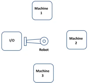
In this problem, there is an in-line robotic cell consisting of m-machines and a robot performing handling operations. The in-line robotic cell is depicted in Fig-ure 4.1. The problem is finding the processing times of the parts on machines that not only minimize the cycle time, but also simultaneously minimize the to-tal manufacturing cost. We consider cyclic scheduling as most of the studies in robotic cell literature do, and we focus on pure cycles. The definitions and assumptions presented in the previous chapter are used in this section. An addi-tional definition used in this section is presented as follows:

δ : Time taken by the robot to travel between two consecutive machines which is additive. Hence, the travelling time from machine i to machine j is equal to |i − j|δ.

CHAPTER 4. BICRITERIA SCHEDULING IN IN-LINE ROBOTIC CELLS24

Input buffer Machine₁ Machine ₂ Machine Machine Output buffer

Robot Linear Track

1

m − m

Figure 4.1: m-Machine In-Line Robotic Cell

4.1.2

Solution Procedure

In this section, the solution method of the bicriteria problem considered in this study is presented. First, the cycle times of proposed pure cycles Cm

1 and C2m

which are defined in Definitions 4.1 and 4.2 are determined when a processing time vector is given. After that, the lower bound of cycle time for a given processing time and number of machines is determined. Then, the processing time vector which results in the lower bound of total manufacturing cost for a given cycle time level is determined. After that, the nondominated solutions of Cm

1 and

Cm

2 for a given cycle time level are determined. For each cycle time level, the

nondominated solutions of Cm

1 and C2m are compared with the processing time

vector resulting in minimum total manufacturing cost for that cycle time level. It is observed that either Cm

1 or C2m results in the processing time vector which

minimizes total manufacturing cost for the specified cycle time regions. So, it is proved that either Cm

1 or C2m dominates the rest of pure cycles in the described

cycle time regions according to bicriteria objective of minimizing both cycle time and total manufacturing cost simultaneously. The proposed pure cycles are Cm

1

and Cm

2 which are defined by Gultekin et al. [12] as follows:

Definition 4.1. Cm

1 is the robot move cycle in an m-machine robotic cell with

the following activity sequence: L1LmUm−1Lm−1Um−2Lm−2. . . U2L2U1Um.

Definition 4.2. Cm

CHAPTER 4. BICRITERIA SCHEDULING IN IN-LINE ROBOTIC CELLS25

the following activity sequence: L1UmLmUm−1Lm−1. . . U2L2U1.

In the initial state of the cycle Cm

1 , the machines 1 and m are idle and the

rest of the machines 2 to m − 1 are already loaded with a part. In the initial state of the cycle Cm

2 , only machine 1 is idle and the rest of the machines 2 to m

are loaded with a part.

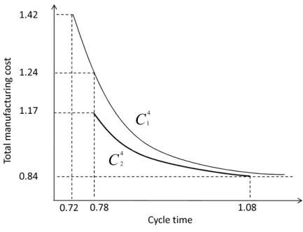
The controllable processing times increase the solution flexibility such that they result in at most equal cost to fixed processing times for a given cycle time level K. The following example is useful to see the contribution of controllable processing times, in order to decrease the total manufacturing cost, compared to fixed processing times for cycle Cm

2 . The total manufacturing cost of cycle C2m

with controllable processing times, which is studied in this study, is compared to the total manufacturing cost of Cm

2 in Gultekin et al. [12], where the

pro-cessing times on machines are assumed to be fixed and same for all machines. In this example, we refer to some lemmas described in the further parts of this study. Example 4.1 There is a 3-machine robotic cell. We will show that the cycle C3

2 with controllable processing times results in less cost than cycle C23 with fixed

processing times for the same cycle time level. Let ² = 0.2, δ = 0.1, PL _{= 2.0,}

PU _{= 4.0. Now, we will compare the processing time vector obtained from}

con-trollable processing times with the processing time vector obtained from fixed processing times, for C3

2.

The processing times are fixed and equivalent in the study of Gultekin et al. [12]. Let us take fixed processing time as P = PL= 2.0, for all machines. Now we

can state the processing time vector with fixed processing times as Pf ixed(C23) =

(2.0, 2.0, 2.0). The cycle time of Cm

2 is denoted by the following equation in

Gultekin et al. [12]: TCm

2 = 4m² + 2((m + 1)

2_{− 2)δ + max{0, P − ((4m − 4)² + 2(m − 1)(m + 2)δ)}}

For the given parameters the cycle time of C3

2 with fixed processing time P = 2.0

is calculated as: T_C3

CHAPTER 4. BICRITERIA SCHEDULING IN IN-LINE ROBOTIC CELLS26

For this cycle time level K = 5.2, the nondominated processing time vec-tor giving the minimum total manufacturing cost for cycle C3

2 is found by using

Lemma 4.5. The nondominated processing time vector (P∗

1, P2∗, P3∗) ∈ P∗(C23|5.2) is defined as follows: P∗_(C3 2|5.2) =     P∗ 1 P∗ 2 P∗ 3     =     min{PU_{, K − (4² + (2m + 2)δ)}} min{PU_{, K − (4² + (2m + 2)δ)}} min{PU_{, K − (4² + (2m + 2)δ)}}     =     min{4.0, 3.6} min{4.0, 3.6} min{4.0, 3.6}     This simply leads to,

P∗_(C3 2|5.2) =     3.6 3.6 3.6    

Now we can compare the processing time vectors for these two cases as:

Pf ixed(C23) =     P P P     =     2.0 2.0 2.0     <     3.6 3.6 3.6     =     P∗ 1 P∗ 2 P∗ 3     = P∗(C23|5.2)

Since the nondominated processing time vector of cycle C3

2 with controllable

processing times is greater than the processing time vector with fixed process-ing times, the cycle C3

2 with controllable processing times results in less total

manufacturing cost.

From now on, we find the cycle times, in Lemmas 4.1 and 4.2, and the set of nondominated points obtained from these two cycles, in Lemmas 4.4 and 4.5, re-spectively for cycle Cm

1 and C2m. Finally, the performances of these two prominent

cycles are compared to the other pure cycles, in Theorems 4.2 and 4.3. Hence, the sufficient conditions under which one of these two cycles dominates the rest of pure cycles are found.

In the following lemma, the cycle time of the first pure cycle Cm

1 is

deter-mined. When there is a given processing time vector, Lemma 4.1 determines the corresponding cycle time obtained from cycle Cm

1 . Conversely, for a specified

cycle time level, the highest processing times on machines that do not violate this cycle time level can be found. Since our aim is to determine the processing times

CHAPTER 4. BICRITERIA SCHEDULING IN IN-LINE ROBOTIC CELLS27

giving minimum manufacturing cost and since cost decreases as processing time increases, this lemma is useful in finding the efficient set of solutions for Cm

1 .

Lemma 4.1. The cycle time of Cm

1 for a given processing time vector is found

as follows: TCm 1 = 4m² + 2m(m + 1)δ + max{0, P1− ((4m − 6)² + 2(m 2_{− 2)δ), P} m− ((4m − 6)² + 2(m2_{− 2)δ), P} kmax− ((4m − 4)² + 2(m2− 1)δ)} kmax = argmax{Pi : i ∈ [2, . . . , m − 1]}.

Proof. Gultekin et al. [12] defined the cycle time of Cm

1 as the total time

re-quired for all of the robot activities and the waiting times in front of the machines and denoted the cycle time as follows:

TCm

1 = 4m² + (2m

2_{+ 2m)δ + w}

1+ w2+ . . . + wm (4.1)

For an m-machine cell, the robot travel time between consecutive machines (δ), the load/unload time of machines (²), and the number of machines (m) are con-stant. Thus, we only have to find the total waiting times in front of the machines to calculate the cycle time. The time between loading machine i and the arrival time of the robot in front of the machine i to unload it is denoted as vi. If

the processing time on machine i, Pi, exceeds vi, then the waiting time is the

difference between Pi and vi. Otherwise, the process on the machine is already

finished when the robot comes to machine i to unload it. Hence, the waiting time of machine i is defined as wi = {0, Pi− vi}. We borrow the below definitions of

vi from Gultekin et al. [12].

v1 = TCm 1 −(6²+(2m+4)δ +w1+wm) = (4m−6)²+(2m 2_{−4)δ +w} 2+. . .+wm−1. vm = TCm 1 −(6²+(2m+4)δ +wm) = (4m−6)²+(2m 2_{−4)δ +w} 1+w2+. . .+wm−1.

In addition, the vi definition for i ∈ [2, . . . , m − 1] is presented as:

vi = TCm

1 − (4² + (2m + 2)δ + wi) = (4m − 4)² + (2m

2_{− 2)δ + w}

1+ . . . + wm− wi.

If there is no waiting time on none of the machines, w1+ w2+ . . . + wm = 0.

If there is waiting time on machine 1, then: w1+ w2+ . . . + wm = P1− v1+

P

j6=1wj = P1− (4m − 6)² − (2m2− 4)δ + wm.

If there is waiting time on machine i where i ∈ [2, . . . , m − 1], then: w1+ w2+ . . . + wm = Pi− vi+

P

j6=iwj = Pi− (4m − 4)² − (2m2 − 2)δ.

CHAPTER 4. BICRITERIA SCHEDULING IN IN-LINE ROBOTIC CELLS28

w1+ w2+ . . . + wm = Pm− vm+

P

j6=mwj = Pm− (4m − 6)² − (2m2− 4)δ.

There are four different cases for the total waiting times and the sufficient condi-tions for these cases are determined as follows:

1. If Pi ≤ vi, ∀i ∈ [1, . . . , m], then wi = 0, for i = 1, . . . , m.

2. Else if Pkmax > vkmax , then wkmax = Pkmax − vkmax = Pkmax − (4m − 4)² −

(2m2_{− 2)δ −}P

i6=kmaxwi. Hence, w1+ w2+ . . . + wm = Pkmax− (4m − 4)² −

(2m2_{− 2)δ.}

3. Else if Pm > vm, then wm = Pm − vm = Pm− (4m − 6)² − (2m2− 4)δ −

P

i6=mwi. Hence, w1+ w2+ . . . + wm= Pm− (4m − 6)² − (2m2− 4)δ.

4. Else if only P1 > v1, then wm = 0 and w1 = P1−v1 = P1−(4m−6)²−(2m2−

4)δ −P_i6=1,mwi. Hence, w1+ w2+ . . . + wm = P1− (4m − 6)² − (2m2− 4)δ.

As a consequence, total waiting time is calculated as:

w1+ w2+ . . . + wm = max{0, P1− ((4m − 6)² + (2m2− 4)δ), Pm− ((4m − 6)² +

(2m2_{− 4)δ), P}

kmax − ((4m − 4)² + (2m2− 2)δ)}.

The cycle time of Cm

1 is obtained by replacing the total waiting time in the

equation (4.1) with this max function. In Lemma 4.2, the cycle time of Cm

2 is determined. When there is a given

processing time vector, Lemma 4.2 gives the corresponding cycle time. Similar to Lemma 4.1, Lemma 4.2 can be used to determine the largest feasible processing times for a given cycle time level.

Lemma 4.2. The cycle time of Cm

2 for a given processing time vector is found

as follows: TCm 2 = 4m² + 2((m + 1) 2_{− 2)δ + max{0, P} kmax− ((4m − 4)² + 2(m − 1)(m + 2)δ)}, kmax = argmax{Pi : i ∈ [1, . . . , m]}.

Proof. Gultekin et al. [12] defined the cycle time of the second pure cycle Cm 2 as follows: TCm 2 = 4m² + (2m 2_{+ 4m − 2)δ + w} 1+ w2 + . . . + wm. (4.2)

CHAPTER 4. BICRITERIA SCHEDULING IN IN-LINE ROBOTIC CELLS29

The total waiting time have to be found in order to calculate the cycle time of Cm

2 corresponding to a processing time. The waiting time on machine i is defined

as wi = {0, Pi− vi}. The definition of vi for all machines is identical for C2m and

it is presented by Gultekin et al. [12] as: vi = TCm

2 −(4²+(2m+2)δ+wi) = (4m−4)²+2(m−1)(m+2)δ+w1+. . .+wm−wi.

If there is no waiting time on none of the machines, then w1+ w2+ . . . + wm = 0.

If there is some waiting time on some machine i, then: w1+ w2+ . . . + wm= Pi− vi+

P

j6=iwj = Pi− (4m − 4)² − 2(m − 1)(m + 2)δ, ∀i.

There are two different total waiting time results and the sufficient conditions for these cases are determined as follows:

1. If Pi ≤ vi for ∀i ∈ [1, . . . , m], then wi = 0, for i = 1, . . . , m

2. Else if Pkmax > vkmax, then wkmax = Pkmax − vkmax = Pkmax − (4m − 4)² −

2(m − 1)(m + 2)δ −P_i6=kmaxwi. Hence, the total waiting time is as follows:

w1+ w2+ . . . + wm = Pkmax− ((4m − 4)² + 2(m − 1)(m + 2)δ).

So, w1+ w2+ . . . + wm = max{0, Pkmax− (4m − 4)² − 2(m − 1)(m + 2)δ} and the

cycle time is obtained by replacing the total waiting time in the equation (4.2) with this max function.

In the next theorem, the lower bound for the cycle time of pure cycles with controllable processing times is defined. The lower bound of cycle time for pure cycles is determined by using Theorem 4.1, when a processing time vector is given.

Theorem 4.1. For an m-machine robotic cell with controllable processing times, the cycle time of any pure cycle is no less than

Tcontr = max{4m² + 2m(m + 1)δ, 4² + (2m + 2)δ + max{Pi, i : 1, . . . , m}}. (4.3)

Proof. From the definition of pure cycles, we determine that the cycle time of a pure cycle has to be greater than or equal to two lower bounds. The first lower bound is obtained from the exact robot activity time and the second one is obtained from the given processing time vector. Since the robot has to perform an

CHAPTER 4. BICRITERIA SCHEDULING IN IN-LINE ROBOTIC CELLS30

exact set of robot activities, the total time required for these activities constitutes a lower bound. Thus, the first lower bound is obtained as follows: The set of robot activities can be analyzed in two groups, the first group consists of robot loading and unloading times. First, a part is taken from the input buffer (²) then loaded to one of the machines (²) after the processing on the machine is finished, the part is unloaded (²) and dropped to the output buffer (²). This makes a total of 4m² time units for a cycle. The robot travel times constitute the second group of robot activities. For any part, the robot takes the part from input buffer to output buffer ((m + 1)δ). Then, the robot travels from the output buffer to input buffer to take a new part or to complete the cycle ((m + 1)δ). This makes a total of 2m(m + 1)δ time units for a cycle. Consequently, the first lower bound, which is the total time required to complete the set of robot activities, makes a total of 4m²+2m(m + 1)δ.

The second lower bound is the minimum time between two consecutive load-ings of any machine. The minimum time needed to unload machine i after loading it is Pi time units. After the processing on the part is finished, it is unloaded (²),

the part is transferred to output buffer ((m+1−i)δ), and the part is dropped (²). After that, the robot travels to the input buffer to take a new part to make the consecutive loading of machine i ((m + 1)δ), takes a new part part, (²), brings the new part to machine i (iδ) and finally loads the machine (²). Hence, the minimum time required between two consecutive loadings of machine i is 4²+(2m+2)δ +Pi.

However there are m machines and the processing times on these machines may be different from each other, due to controllability. Thus, the cycle time has to be at least equal to the minimum time required between two consecutive load-ings of any machine in the cell. So, the second lower bound of the cycle time is 4² + (2m + 2)δ + max{Pi, i : 1, . . . , m}.

Our aim is to determine the processing time vector providing the minimum cost for a given cycle time level. The total manufacturing cost depends only on the processing times on machines. The manufacturing cost of a machine decreases as the processing time increases on that machine. A feasible processing time must satisfy PL_{≤ P}

i ≤ PU. Since PL constrains processing time from below and our

CHAPTER 4. BICRITERIA SCHEDULING IN IN-LINE ROBOTIC CELLS31

to involve PL_{in analysis as a constraint. A processing time vector is composed of}

processing times on machines constrained by two bounds. For any pure cycle, the processing time on any machine is bounded above by the processing time upper bound PU_{. In addition, from Theorem 4.1, processing times are bounded by cycle}

time level K. Consequently, for a given cycle time level, we can find the upper bounds of processing times for pure cycles that do not violate this cycle time level. After obtaining these two bounds for processing times on all machines, the upper bound of processing time vectors is determined for pure cycles. In other words, any pure cycle cannot have a greater processing time vector than the proposed processing time vector of the next lemma. Since this processing time vector is an upper bound for the processing time vectors obtained from pure cycles for a cycle time level K, it also results in the lower bound of total manufacturing cost that a pure cycle can result in. Let P(K) = (P1(K), . . . , Pm(K)) denote the upper

bound of processing time vectors. Now, P(K) for a given cycle time level K is found as follows:

Lemma 4.3. For a given cycle time level K, the upper bound of processing time vectors for pure cycles is represented as follows:

P(K) = (P1(K), . . . , Pm(K)), where Pi(K) = min{PU, K −(4²+(2m+2)δ)},∀i.

Proof. The two bounds constraining processing time vectors are found in the following cases.

1. The processing time on any machine is less than PU_{. This leads to:}

Pi(K) ≤ PU, ∀i.

2. In addition, the processing times on the machines cannot exceed a specific value, since otherwise the cycle time level K will be exceeded. Now, we find the upper bound of processing time on machine i, Pi, for the cycle time

level K. Theorem 4.1 determines the lower bound for the cycle time, when a processing time vector is given. The cycle time lower bound in Theorem 4.1 is presented as: