INTRADAY LEAD-LAG RELATIONSHIP BETWEEN WARRANTS AND
FUTURES CONTRACTS: A CASE OF ISE-30 STOCK INDEX
DENİZ AKÇALI
108673066
İSTANBUL BİLGİ ÜNİVERSİTESİ
SOSYAL BİLİMLER ENSTİTÜSÜ
BANKACILIK VE FİNANS YÜKSEK LİSANS PROGRAMI
NURGÜL CHAMBERS
2012
INTRADAY LEAD-LAG RELATIONSHIP BETWEEN WARRANTS AND
FUTURES CONTRACTS: A CASE OF ISE-30 STOCK INDEX
VARANT VE FUTURES SÖZLEŞMELERİ ARASINDAKİ GÜNİÇİ
ÖNCÜL-ARDIL İLİŞKİSİ :
DENİZ AKÇALI
108673066
Prof. Dr. Nurgül Chambers
:...
Yard. Doç. Cenktan Özyıldırım
:...
Mehmet Hakan Şengöz
:...
Tezin Onaylandığı Tarih
: ...
Toplam Sayfa Sayısı:120
Anahtar Kelimeler (Türkçe) Anahtar Kelimeler (İngilizce)
1)
Varant
1) Warrant
2)
Vadeli İşlem
2) Futures
3)
Gün içi Öncül-Ardıl
3) Lead-Lag
4)
Vektör Otoregresif
4) Vector Autoregression
iii
ABSTACT
The aim of this thesis is to investigate empirically the intraday lead-lag relationship between warrants and futures market as applied to those traded at the Istanbul Stock Exchange (ISE) and Turkish Derivatives Exchange (Turkdex). Focus is used an intuitive method to examine the intraday lead-lag relation, if any, in the high frequency intraday data of warrants and futures which have same underlying stocks index using parametric and nonparametric methods at 5-minutes regular time interval.
The data set for the study consists of the 5 minutes time interval closing values of the ISE 30 index futures traded at the Turkdex and ISE 30 index put and call warrants traded at ISE and issued by Deutsche Bank, which are considered from January 6, 2012 to February 29, 2012 period; from May 8, 2012 to June 29, 2012 period and from July 2, 2012 to August 31, 2012 for near month futures contracts, near month and mostly heavily traded put and call warrants.
As parametric methods, cross correlation functions and Granger causality model are used to investigate whether a short term relationship among the time exists or not and vector autoregressive model is used to examine the short-term relationship between future contracts and warrants. Impulse-response functions and variance decomposition methods are also used as complementary methods to show the effects of the change in the error terms of the variables in the study on the other variables. Counting method is used as non-parametric method and statistically significance of its results is tested by chi-square method.
We find that both parametric method's and non-parametric counting method's results shows that there is an evidence that futures contract market lead the
iv warrant markets in Turkey. On the contrary, warrants do not lead futures market. This result is statistically significant.
v
ÖZET
Bu çalışmanın amacı, dayanak varlığı İMKB-30 hisse senedi endeksi olan, İMKB’de işlem gören varant ve VOB’da işlem gören futures sözleşmeleri arasındaki gün içi öncül-ardıl ilişkisini araştırmaktır. Çalışmada, aynı dayanak varlığa sahip varant ve vadeli işlem sözleşmeleri arasındaki öncül-ardıl ilişkisinin 5’er dakikalık zaman aralıklarıyla temin edilen kotasyon verileri ile incelenmesine odaklanılmıştır.
Çalışmada, 06.01.2012-29.02.2012, 08.05.2012 ve 02.07.2012-31.08.2012 tarihleri için İMKB-30 endeksine dayalı vadeli işlem sözleşmeleri ile alım satım varantlarının kapanış fiyatları kullanılmış, en çok işlem gören varantlar ile varantların vadesine yakın vade sonu olan futures sözleşmeler seçilmiştir. Parametrik yöntemler kapsamında, çapraz korelasyon ve Granger Nedensellik Testleri ile Vektör Otoregresyon Modeli ile varantlar ve futures sözleşmeler arasındaki kısa dönemli ilişki analiz edilmiştir. Etki tepki fonksiyonları ile varyans ayrıştırma metotları uygulanmış ve hata terimindeki değişimler analiz edilmiştir. Parametrik olmayan sayma metodu uygulanmış, istatistiksel anlamlılığı Ki-Kare Testi ile ölçülmüştür.
Gerek parametrik gerekse parametrik olmayan yöntemlerin sonuçları, Türkiye’de futures sözleşmelerin işlem gördüğü piyasaların varant piyasasına öncülük ettiği yönünde bulgular sunmuştur. Diğer yandan, varant piyasasına öncülük ettiği yönünde bir kanıta rastlanmamıştır. Elde edilen sonuçlar istatistiksel olarak anlamlı bulunmuştur.
vi TABLE OF CONTENTS ABSTACT ... iii ÖZET ... v TABLE OF CONTENTS ... vi LIST OF TABLES ... ix LIST OF FIGURES ... xi 1.INTRODUCTION ... 13 2.LITERATURE REVIEW ... 15 3.WARRANTS ... 22 3.1. Definition of Warrant ... 22 3.2. Features of Warrants ... 22
3.2.1. Underlying Instruments of Warrants ... 22
3.2.2. Types of Warrants ... 23
3.2.3. Exercise Price of Warrants ... 24
3.2.4. Expiry Date and Exercise Style of Warrants ... 25
3.2.5. Conversion of Warrants ... 25
3.3. Value Term in Warrant Features ... 26
3.4. General Overview of Models Used for Valuation of Warrants ... 28
3.4.1. Black-Scholes-Merton European Call Option Model ... 28
3.4.2. Dilution-Adjusted Black-Scholes-Merton Model ... 29
3.5. Factors Influencing The Warrant Price ... 29
3.5.1. Price of the Underlying Asset of Warrant ... 30
3.5.2. Exercise Price of Warrant ... 30
3.5.3. Days to Maturity for Warrant ... 30
3.5.4. Volatility of Underlying asset ... 30
3.5.5. Market Interest Rate ... 30
3.5.6. Dividend of the company ... 30
vii
3.6.1. Advantages ... 31
3.6.2. Disadvantages ... 33
3.7. Comparison of Warrants and Options ... 34
3.7.1. Similarities ... 34
3.7.2. Differences ... 34
3.8. Turkish Warrant Market... 35
3.8.1 Legal Grounds for Turkish Warrant Market ... 35
3.8.2 Features of Warrants To Be Traded ... 36
3.8.3. Transaction Code of Warrants ... 37
3.8.4 Operation of Warrant Market ... 37
3.8.4 General Rules for Warrant Market Maker ... 39
3.8.6 Settlement and Conversion Transactions of Warrants ... 40
3.8.5 General Overview of The Warrant Market in Turkey ... 42
4.FUTURES CONTRACTS ... 47
4.1 Brief Information About Futures Contracts ... 47
4.2 Turkish Derivatives Exchange ... 48
4.3 Specifications of ISE-30 Future Contracts... 49
5.METHODOLOGY ... 50
5.1. Data ... 50
5.2. Parametric Method ... 51
5.2.1. Cross Correlation Function ... 51
5.2.2. Vector Autoregression Model ... 52
5.2.3. Granger Causality ... 52
5.2.4. Impulse Response Functions... 53
5.2.5. Variance Decomposition ... 54
5.3. Non-Parametric Counting Method ... 55
6.EMPRICAL RESULT ... 58
6.1. Descriptive Statistics ... 58
6.2. Unit Root Test ... 59
6.3. Cross Correlation Function ... 61
6.4. VAR Model ... 62
viii
6.6. Impulse Response Function ... 76
6.7. Variance Decomposition ... 83
6.8. Nonparametric Counting Method ... 84
7.CONCLUSION ... 89
REFERENCES ... 93
APPENDICES ... 99
A.Time Series of Natural Algorithm of Selected Future Contracts and Warrants ... 99
B.Descriptive Analysis of Return Series of Selected Future Contracts and Warrants ... 101
C.Times Series of Natural Logarithmic Return Series of Selected Future Contracts and Warrants ... 102
D.Frequency Distribution of Logarithmic Return Series of Selected Future Contracts and Warrants ... 104
E.Cross Correlation Functions Between Each Warrant And Future ... 106
F.Cross Correlogram Results of Each Pair of Warrant and Future Contract….. ... 109
G.Optimal Lag Length Selection Tables According to Akaike Information Criteria (AIC), Schwarz Information Criteria (SIC) and Hannan Quinn Criteria (HQ) ... 113
H.Variance Decomposition Tables Between Selected Futures and Warrants ... 117
LIST OF TABLES
Table 1. Numbers of issued warrants and investors and trading volume in Turkey's
warrants market ... 43
Table 2. Warrants Trading Volume and Numbers According to Investor Type in Turkey's warrants market ... 43
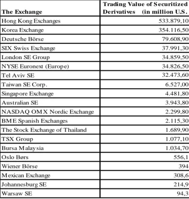
Table 3. Total Transaction Volume Rankings in Turkish Warrant Market ... 44
Table 4. Trading value of securitized derivatives in the worldwide exchanges in 2010 ... 45
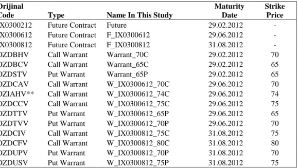
Table 5. List of Warrants and Futures Contracts Used in the Study ... 50
Table 6. ADF Test Results ... 60
Table 7. Results of Cross Correlation Analyses ... 62
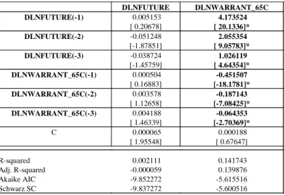
Table 8. VAR model results for DLFUTURE and DLWARRANT_70C ... 63
Table 9. VAR model results for DLFUTURE and DLWARRANT_65C ... 64
Table 10. VAR model results for DLFUTURE and DLWARRANT_65P ... 65
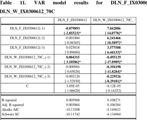
Table 11. VAR model results for DLN_F_IX0300612 and DLN_W_IX0300612_70C ... 66
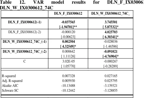
Table 12. VAR model results for DLN_F_IX0300612 and DLN_W_IX0300612_74C ... 67
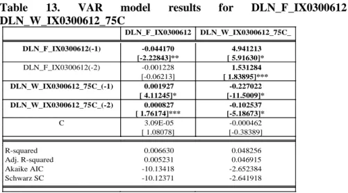
Table 13. VAR model results for DLN_F_IX0300612 and DLN_W_IX0300612_75C ... 68
Table 14. VAR model results for DLN_F_IX0300612 and DLN_W_IX0300612_65P ... 68
Table 15. VAR model results for DLN_F_IX0300612 and DLN_W_IX0300612_70P ... 69
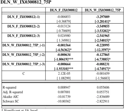
Table 16. VAR model results for DLN_F_IX0300812 and DLN_W_IX0300812_75C ... 70
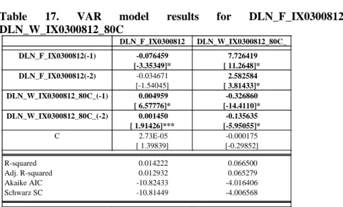
Table 17. VAR model results for DLN_F_IX0300812 and DLN_W_IX0300812_80C ... 71
Table 18. VAR model results for DLN_F_IX0300812 and DLN_W_IX0300812_70P ... 72
Table 19. VAR model results for DLN_F_IX0300812 and DLN_W_IX0300812_75P ... 73
Table 20. Granger cause test results for Jan 6 - Feb 29, 2012 period ... 74
Table 21. Granger cause test results for May 8 - Jun 29, 2012 period ... 74
Table 22. Granger cause test results for Jul 2 - Aug 31, 2012 period ... 75
Table 23. Results of Nonparametric Counting Method for Jan 6 - Feb 29, 2012 period ... 85
Table 24. Chi-square test of Nonparametric Counting Method for Jan 6 - Feb 29, 2012 period ... 85
Table 25. Results of Nonparametric Counting Method for May 8 - Jun 29, 2012 period ... 86
Table 26. Chi-square test of Nonparametric Counting Method for May 8 - Jun 29, 2012 period ... 86
Table 27. Results of Nonparametric Counting Method for Jul 2 - Aug 31, 2012 period ... 87
Table 28. Chi-square test of Nonparametric Counting Method for Jul 2 - Aug 31, 2012 period ... 88
Table 29. Descriptive statistics of natural logarithmic return series of selected futures and warrants index prices between Jan 6 - Feb 29, 2012 ... 101
x Table 30. Descriptive statistics of natural logarithmic return series of selected futures and warrants index prices between May 8 - Jun 29, 2012 ... 101 Table 31. Descriptive statistics of natural logarithmic return series of selected futures and warrants index prices between Jul 2 - Aug 31, 2012 ... 101 Table 32. Optimal lag selection test results for DLFUTURE and
DLWARRANT_70C ... 113 Table 33.Optimal lag selection test results for DLFUTURE and
DLWARRANT_65C ... 113 Table 34. Optimal lag selection test results for DLFUTURE and
DLWARRANT_70C ... 113 Table 35. Optimal lag selection test results for DLN_F_IX0300612 and
DLN_W_IX0300612_70C ... 114 Table 36. Optimal lag selection test results for DLN_F_IX0300612 and
DLN_W_IX0300612_74C ... 114 Table 37. Optimal lag selection test results for DLN_F_IX0300612 and
DLN_W_IX0300612_75C ... 114 Table 38. Optimal lag selection test results for DLN_F_IX0300612 and
DLN_W_IX0300612_65P ... 115 Table 39. Optimal lag selection test results for DLN_F_IX0300612 and
DLN_W_IX0300612_65P ... 115 Table 40. Optimal lag selection test results for DLN_F_IX0300812 and
DLN_W_IX0300812_75C ... 115 Table 41. Optimal lag selection test results for DLN_F_IX0300812 and
DLN_W_IX0300812_80C ... 116 Table 42. Optimal lag selection test results for DLN_F_IX0300812 and
DLN_W_IX0300812_70P ... 116 Table 43. Optimal lag selection test results for DLN_F_IX0300812 and
DLN_W_IX0300812_75P ... 116 Table 44. Variance Decomposition of DLFUTURE and DLWARRANT_70C .. 117 Table 45. Variance Decomposition of DLFUTURE and DLWARRANT_65C .. 117 Table 46. Variance Decomposition of DLFUTURE and DLWARRANT_65P ... 117 Table 47. Variance Decomposition of DLN_F_IX0300612 and
DLN_W_IX0300612_70C ... 118 Table 48. Variance Decomposition of DLN_F_IX0300612 and
DLN_W_IX0300612_74C ... 118 Table 49. Variance Decomposition of DLN_F_IX0300612 and
DLN_W_IX0300612_75C ... 118 Table 50. Variance Decomposition of DLN_F_IX0300612 and
DLN_W_IX0300612_65P ... 119 Table 51. Variance Decomposition of DLN_F_IX0300612 and
DLN_W_IX0300612_70P ... 119 Table 52. Variance Decomposition of DLN_F_IX0300812 and
DLN_W_IX0300812_75C ... 119 Table 53. Variance Decomposition of DLN_F_IX0300812 and
DLN_W_IX0300812_80C ... 120 Table 54. Variance Decomposition of DLN_F_IX0300812 and
DLN_W_IX0300812_70P ... 120 Table 55. Variance Decomposition of DLN_F_IX0300812 and
DLN_W_IX0300812_75P ... 120
LIST OF FIGURES
Figure 1. Popular underlying financial products for writing warrants ... 23
Figure 2. Time value and intrinsic value of a call warrant ... 27
Figure 3. Turkish Warrant Market Session Hours ... 38
Figure 4. Trading Volume of ISE-30 Index Futures Contracts ... 48
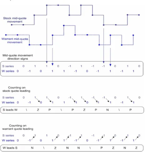
Figure 5. The algorithm of Kui (2007)'s counting methods to detect the lead-lag relationships between warrants and their underlying stocks ... 55
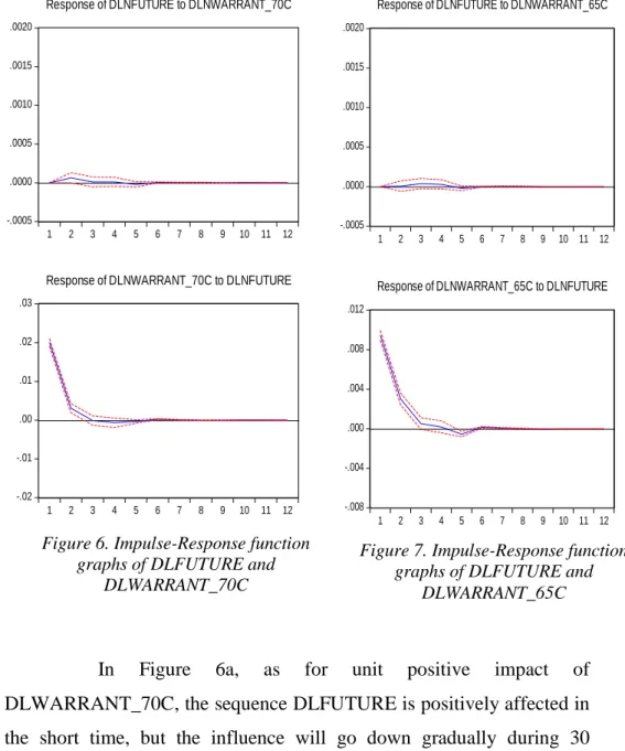
Figure 6. Impulse-Response function graphs of DLFUTURE and DLWARRANT_70C... 77
Figure 7. Impulse-Response function graphs of DLFUTURE and DLWARRANT_65C... 77
Figure 8. Impulse-Response function graphs of DLN_F_IX0300612 and DLN_W_IX0300612_70C ... 78
Figure 9. Impulse-Response function graphs of DLFUTURE and DLWARRANT_65P ... 78
Figure 10. Impulse-Response function graphs of DLN_F_IX0300612 and DLN_W_IX0300612_74C ... 79
Figure 11. Impulse-Response function graphs of DLN_F_IX0300612 and DLN_W_IX0300612_75C ... 79
Figure 12. Impulse-Response function graphs of DLN_F_IX0300612 and DLN_W_IX0300612_65P ... 80
Figure 13. Impulse-Response function graphs of DLN_F_IX0300612 and DLN_W_IX0300612_70P ... 80
Figure 14. Impulse-Response function graphs of DLN_F_IX0300812 and DLN_W_IX0300812_75C ... 81
Figure 15. Impulse-Response function graphs of DLN_F_IX0300812 and DLN_W_IX0300812_80C ... 81
Figure 16. Impulse-Response function graphs of DLN_F_IX0300812 and DLN_W_IX0300812_70P ... 82
Figure 17. Impulse-Response function graphs of DLN_F_IX0300812 and DLN_W_IX0300812_75P ... 82
Figure 18. Time series of natural logarithm of selected futures and warrants index prices between Jan 6 - Feb 29, 2012 ... 99
Figure 19. Time series of natural logarithm of selected futures and warrants index prices between May 8 - Jun 29, 2012 ... 100
Figure 20. Time series of natural logarithm of selected futures and warrants index prices between Jul 2 - Aug 31, 2012 ... 100
Figure 21. Time series of natural logarithmic return series of selected futures and warrants index prices between Jan 6 - Feb 29, 2012 ... 102
Figure 22. Time series of natural logarithmic return series of selected futures and warrants index prices between May 8 - Jun 29, 2012 ... 102
Figure 23. Time series of natural logarithmic return series of selected futures and warrants index prices between Jul 2 - Aug 31, 2012 ... 103
Figure 24. Frequency distributions of natural logarithmic return series of selected futures and warrants index prices between Jan 6 - Feb 29, 2012 ... 104
Figure 25. Frequency distributions of natural logarithmic return series of selected futures and warrants index prices between May 8 - Jun 29, 2012 ... 104
Figure 26. Frequency distributions of natural logarithmic return series of selected futures and warrants index prices between May 8 - Jun 29, 2012 ... 105
xii
Figure 27. Cross Correlation between DLFUTURE and DLWARRANT70C
between Jan 6 - Feb 29, 2012 ... 106 Figure 28. Cross Correlation between DLFUTURE and DLWARRANT65C
between Jan 6 - Feb 29, 2012 ... 106 Figure 29. Cross Correlation between DLFUTURE and DLWARRANT65P
between Jan 6 - Feb 29, 2012 ... 106 Figure 30. Cross Correlation between DLN_F_IX0300612 with
DLN_W_IX0300612_70C between May 8 - Jun 29, 2012 ... 106 Figure 31. Cross Correlation between DLN_F_IX0300612 with
DLN_W_IX0300612(74C) between May 8 - Jun 29, 2012 ... 107 Figure 32. Cross Correlation between DLN_F_IX0300612 with
DLN_W_IX0300612(75C) between May 8 - Jun 29, 2012 ... 107 Figure 33. Cross Correlation between DLN_F_IX0300612 with
DLN_W_IX0300612_65P between May 8 - Jun 29, 2012 ... 107 Figure 34. Cross Correlation between DLN_F_IX0300612 with
DLN_W_IX0300612_70P between May 8 - Jun 29, 2012 ... 107 Figure 35. Cross Correlation between DLN_F_IX0300812 with
DLN_W_IX0300812_75C between Jul 2 - Aug 31, 2012 ... 108 Figure 36. Cross Correlation between DLN_F_IX0300812 with
DLN_W_IX0300812_80C between Jul 2 - Aug 31, 2012 ... 108 Figure 37. Cross Correlation between DLN_F_IX0300812 with
DLN_W_IX0300812_70P between Jul 2 - Aug 31, 2012 ... 108 Figure 38. Cross Correlation between DLN_F_IX0300812 with
DLN_W_IX0300812_75P between Jul 2 - Aug 31, 2012 ... 108 Figure 39. Cross Correlogram between DLFUTURE and DLWARRANT65P .... 109 Figure 40. Cross Correlogram between DLFUTURE and DLWARRANT65C .... 109 Figure 41. Cross Correlogram between DLFUTURE and DLWARRANT70C .... 109 Figure 42. Cross Correlogram between DLN_F_IX0300612 and
DLN_W_IX0300612_70P ... 110 Figure 43. Cross Correlogram between DLN_F_IX0300612 and
DLN_W_IX0300612_75C ... 110 Figure 44. Cross Correlogram between DLN_F_IX0300612 and
DLN_W_IX0300612_74C ... 110 Figure 45. Cross Correlogram between DLN_F_IX0300612 and
DLN_W_IX0300612_65P ... 111 Figure 46. Cross Correlogram between DLN_F_IX0300612 and
DLN_W_IX0300612_70C ... 111 Figure 47. Cross Correlogram between DLNF_IX0300812 and
DLN_W_IX0300812_70P ... 111 Figure 48. Cross Correlogram between DLNF_IX0300812 and
DLN_W_IX0300812_75C ... 112 Figure 49. Cross Correlogram between DLNF_IX0300812 and
DLN_W_IX0300812_80C ... 112 Figure 50. Cross Correlogram between DLNF_IX0300812 and
13
1.INTRODUCTION
A warrant is a right to purchase or sell, within a specified period, a share of common stock at a specified price. The definition is so similar to that of the call options. The economic function of warrants is no different from options. These derivatives are leveraged securities that give investors the exposure to the underlying assets at a fraction of the cost, and the opportunity to enjoy geared returns when the market moves in favour, or to limit and hedge the risk of an existing portfolio in a falling market.
Despite their similarities, there are some important differences between call options and warrants. First, while the call option is issued by an individual, the warrant is issued by the firms. If a warrant is exercised, it increases the number of outstanding shares of the firm and thus dilutes the equity of the company while call options don’t increase share numbers when call options are exercised more elaborately. Second, while call options expire within several months, warrants typically have maturities of at least several years.
This thesis tries to give some information about development process of Turkish Warrant Market and address the question concerning the lead-lag relation between the index warrant and index futures which have same underlying asset. The objective of this study is to address the question of whether there is any lead-lag relationship between stock index warrants and stock index futures in Turkey or not.
This thesis contributes to the literature in three aspects. First, we analyze short term dynamics between future contracts and warrants via parametric methods. In this way, lead-lag relationship is investigated by cross correlation, granger causality method and vector autoregressive model with complementary analysis of it. Second, we represent a counting method
14 to study the lead‐lag relation between warrants and the underlying security’s futures in Turkey. This method is efficacious in examining the lead‐lag relation at the high frequency with a time resolution of 5 minutes. It is non‐parametric and the assumptions critical to the regression approaches are not needed.
The rest of the thesis is organized as follows. In Chapter One, we present an introduction. Chapter Two provides a literature review. In Chapter Three, we give some information about characteristics and background of the warrants and warrants market in Turkey. In Chapter Four, we present theoretical background about parametric methods: cross-correlation and vector autoregressive model and non-parametric counting method, and documents the data we use in our empirical study. Chapter Five provides an analysis of the lead-lag relation between index futures and index warrants on same underlying stock index - ISE 30 - in Turkey.
15
2.LITERATURE REVIEW
Several studies have provided theoretical models for the pricing of warrants. These include the works of Black and Scholes in 1973, and Galai and Schneller in 1978 and Lauterbach and Schultz in 1990.
Santoso (2000) has mentioned that Black and Scholes claimed that in many cases their model could be used as an approximation to estimate the warrant value. Black-Scholes (1973) first introduced pricing model of options. Kremer (1992) had claimed that the option pricing work of Black-Scholes is known to be motivated by prior research on warrant pricing. Merton (1973) used dividend adjustment to Black-Scholes formula and proposed that when the dividend is paid, stock price decreases. The pricing theories by Black and Scholes (1973) and Merton (1973) indicated that, the price of an option is dependent on its underlying security. Only after the stock price is known can the option price be determined. However, if material information is discovered earlier in the equity option market as a result of the trades by informed traders who want to take advantage of the leverage that options provide, then the option price may lead the underlying stock price. Lauterbach and Schultz (1990) had reached a conclusion that Black and Scholes warned early in 1973 that given the relatively long life of a warrant, the volatility of the underlying stock may be expected to change substantially.
Galai and Schneller (1978) proposed the concept of dilution effect of warrants on the value of firm. The empirical results showed that number of warrants issued would not effect the wealth of shareholders even if issuance of warrants may increase future cash flows, since they would be offset by dilution of number of shares increased as warrants were exercised. Shortly, they regarded a warrant as a diluted option of an identical firm without warrants outstanding. Both studies suggested that any call
option-16 pricing model with some minor modifications could be used to price warrants.
Other empirical studies on warrant pricing include the works of Lauterbach and Schultz (1990), Leonard and Solt (1990), and Hauser and Lauterbach (1997) on U.S. warrants and Schulz and Trautmann (1994) on German warrants. Leonard and Solt (1990) concluded that the Scholes model performs as well as more complicated adjusted Black-Scholes models for warrant pricing. They suggested that for dividend paying firms the dividend-adjusted Black-Scholes model is more accurate than the diluted adjusted one, when warrants are in-the-money or have a long maturity. Schulz and Trautmann, helped to justify option-like warrant valuation ignoring dilution effect. They have argued that dilution adjustment created double counting effects, because stock price has already incorporated dilution effects during the warrant’s life. On the other hand, Lauterbach and Schultz (1990), followed by Hauser and Lauterbach, presented evidence that suggests that the Black-Scholes model be outperformed by a model that assumes a constant elasticity of variance diffusion process for stock price. They constructed the model substituting the equity value into the stock price and adjusting the effect of dilution presented by Galai and Schneller (1978). Schwartz (1977) generalized the Black-Scholes formulation by employing a closed form solution to the differential equation subject to the appropriate boundary conditions that governs the value of a warrant.
Option pricing models that incorporate adjustments to the effect of potential dilution and changing volatility are might be more appropriate for valuing warrants. Santoso (2000) had claimed that several theoretical studies have provided such models, and several empirical researches have tested them based on warrants traded at developed markets, such as U.S. and Europe, as well as at the emerging markets.
In addition to possible dilution, Chan and Pinder (2000) had stated there are other reasons for the difference in prices between warrants
17 and options. They proposed that difference resulted from the credit risk of the issuer of the warrant, since warrants were usually issued by a third party, generally a financial institution. Additionally, they showed that warrant prices reflect the different levels of credit risk associated with warrant issuers in their studies.
Santoso (2000) investigates empirically the relative performance of pricing models commonly used for warrants traded at the Jakarta Stock Exchange. He focuses that warrant pricing models incorporating adjustment for dilution and changing volatility. His finding suggests that dilution adjustment improves the pricing performance of Black-Scholes-Merton model. It is also indicated that models that allow an inverse relation between stock price and volatility might promise superior pricing performance.
Santoso (2000) has mentioned that empirical research on warrants traded at emerging markets includes the work of Shastri and Sirodom (1995) and Kwok (1994). Shastri and Sirodom (1995) concluded that a constant elasticity of variance model outperformed Black-Scholes model in a study about the pricing of Thailand warrants. On the other hand, he had mentioned that Kwok (1994) confirmed the practical efficiency of Hong Kong traded warrant market using Black-Scholes model.
Many analysts, including Mayhew (1995), Easley et al. (1998), have examined the option and stock price behaviors under information asymmetry. They find that informed traders do trade actively in the option market and so, this finding is that, if more informed traders leverage on options to generate a return higher than the return from trading stocks, then the option price will move ahead of the stock price in impounding the information from the informed traders.
Stephan and Whaley (1990) investigated the intraday price change and trading volume relationship between stocks and options by using causality tests causality tests of observed and implied stock prices and found that price changes in the stock market lead the option market by
18 fifteen minutes. However, Manaster and Rendleman (1982) and Anthony (1988) had found a reverse relationship. Manaster and Rendleman (1982) had used daily closing data in their study and found that option market is leading stock prices for 1 day. Anthony (1988) had used daily data to examine by using causality tests to determine timing and direction of information flow. He argued that call options led underlying shares and underlying shares were taken 1 day to adjust price changes in the option. Chan et al. (1993) used a nonlinear multivariate model to compute implied stock prices, rather than an option pricing model and argued that stock price, rather than the transaction price, led the bid-ask midpoint. They have found that neither market led.
Kui (2007) suggests an intuitive method to examine the lead‐lag relation, if any, in the tick‐by‐tick data of covered warrants and their underlying stocks or underlying index futures. Kui find that the electronically traded warrants do not lead stocks or index futures; the movements in the warrants’ quotes provide little information about the quotes of the underlying stocks or index futures. Kui also shows that the stocks and index futures lead the warrants.
There are various studies that have analyzed the lead/lag relation between derivatives and the spot market. However, empirical studies examining the intraday patterns on warrant market is relatively scarce in Turkey, the absence of data in these markets may possibly be a reason for it. Abuk (2011) had claimed that the general consensus reveals that futures market is the leader of both options and and spot markets with little or no feedback. But, there is no consensus for the relation between options and spot markets. Finnerty & Park (1987) and Kawaller et al. (1987) are the first that investigate the temporal relation between index futures and the cash index markets. Both reach to the conclusion that futures market leads the spot market. Kawaller et al. (1987) found that index futures prices lead cash index prices up to 40 minutes although cash index of only one minute is observed at times. In these studies, the price discovery role of futures
19 market mostly had been explained by low transaction costs and high degree of leverage.
Stephan and Whaley (1990) investigated intraday lead-lag relationship between S&P 500 and money market index futures by using data broken into 5 minute intervals. They showed that futures market leads spot market about 5 and 10 minutes but there was no unidirectional effect between them. They also suggested that there was evidence that spot market led the futures market even though it was not a very strong effect respectively.
Frank De Jonga and Monique W.M. Donders (1996) had proposed that investigation of intraday lead-lag relationships between futures, options and underlying index with high frequency data and observations on the three series which are probably unequally spaced in time. They have showed that futures market led both options and the underlying asset’s spot market by using a regressive model which is modified according to covariances and correlations. They have mentioned that choosing a long unit time interval minimizing the number of missing observations and imputing zero returns for intervals in which no trading took place were the two ways to deal with that problem of unequally spaced observations. However, they also mentioned that these methods had 2 shortcomings. First, when a long unit time interval is chosen, trading cannot be very frequent, in which a lot of information is thrown away. Second, there is a risk in imputing zero returns for intervals in which no trading took place that it can create an error in the variables problem that will bias the covariance and correlation estimates toward zero. They have mentioned that in perfectly efficient market, all price movements were expected to be simultaneous and lead-lag relationship existed. They have interpreted the results of their study that quotes of cash index were due to infrequent trading. Moreover, they have claimed that futures market had leverage effect twice as large as in the option market and transaction costs are lower in futures market relative to the option market and the spot market.
20 The relationship between spot and derivatives markets is first studied by Ozen et al. (2009) in Turkey. Futures transactions from Turkish Derivatives Exchange (TURKDEX, VOB) and Istanbul Stock Exchange (ISE) national 30 spot index prices are examined with closing prices of 1.024 trading days for the period February 4, 2005 – February 27, 2009. Their study focused on the short and long run causal relationship on the basis of co-integration and then determines the direction of the relation by Granger causality applied over error correction mechanism. Long run results indicate bidirectional causality whereas a unilateral causality relationship from spot to futures market was determined.
Kapusuzoğlu and Tasdemir (2010) try to explain the impact of TURKDEX futures market on ISE national 100 index prices through market efficiency. Similar to the previous study of Ozen et al. (2009), co-integration and Granger causality are performed on the daily closing prices beginning from November 1, 2005 until June 30, 2009. Empirical study reveals that both TURKDEX derivatives and ISE spot markets are efficient in a weak form. What they find is on the contrary to the expected result of dominant futures market. The futures market price is found to be not effective on the spot market price and spot market is found to be leading futures market significantly. They have interpreted the results of their study that the derivative market in Turkey was not very efficient and increasing volume of transactions in futures contracts and development of the TurkDex would contribute positively to the efficiency.
Öztürk (2008) investigated of ISE-100 index and ISE30 index spot market returns and the returns of futures contracts’ based on these indices. He found in his study that for daily returns of variables there was a one way causality relationship from spot market to futures market.
Kayalıdere (2012) et. al. has aimed to analyze the interaction between derivatives and spot markets using ISE-30, TURKDEX-TL/Dollar futures contracts. Short and long term dynamics between market prices have been researched by the VAR (Vector Autoregressive Regression) Model and
21 it has been concluded that there was an effect from derivatives market to spot market for the latest years while there is an interaction from spot
22
3.WARRANTS
3.1. Definition of Warrant
Warrants are capital markets instruments that give the holders the right to buy or sell the underlying instrument or indicator at a predetermined price on, or before, a particular date, against a premium payment. This right is exercised by registered delivery or cash settlement and this right doesn’t mean an obligation for the holder.
Warrants, which are only under the responsibility of the issuer, are securitized options which are listed on a stock exchange and traded in the relevant market segment. They are traded in the secondary market and settled in the same way like the other securities.
Warrants are known as structured products which are not issued for financing purposes. They derive their value from another underlying instrument. Some warrants give holders the right to buy, or to sell the underlying instrument to the warrant issuer for a particular price according to the terms of issue. Alternatively, some of them such as index warrants provide holders with a cash payment relating to the value of the underlying instrument at a particular time.
3.2. Features of Warrants
Some key warrant features are described below. Warrants do not have standardized terms, since some of them appear in all warrant types and some do not.
3.2.1. Underlying Instruments of Warrants
Warrants can be issued over securities such as shares, a basket of different securities, a share price index, debt, currencies and commodities. Some warrants have higher risk/return profiles than others
23 that offer lower risk features such as capital guarantees. (http://www.macquarie.com.au).
Source: imkb.org.tr
Figure 1. Popular underlying financial products for writing warrants
As shown in the Figure 1 above, the underlying asset may be a single equity or a basket of equities. (For example, call warrant issued by Z bank, entitling the holder to buy the shares of ABC Incorp. at TL 6.00 on 20.12.2014.) If the underlying instrument of a warrant is a single equity or a basket of equities, “underlying asset” term is used, whereas in the case of warrants written on an index, the term “underlying indicator” is used. (For example, a put warrant issued by Z bank, which entitles the holder to sell the ISE-100 Index at 80,500 points on 20.12.2014)
Warrants over a basket of securities give exposure to the performance of a group of securities or a particular industry. The underlying instrument may be adjusted. if there is a corporate action or similar event and the disclosure document would explain when this may occur.
3.2.2. Types of Warrants
Investors use trading warrants to gain significant leveraged exposure to a variety of underlying assets in a rising or falling market. (http://www.asx.com.au/products/about-asx-warrants.htm). Some types of warrants can also be used to protect the value of an existing portfolio or
24 shareholding and they are called as investment warrants. Warrants can be classified as either call warrants or put warrants. Call warrants benefit from an upwards price movement in the underlying instrument whereas put warrants benefit from a downward price movement. Warrants that give the right to buy have the advantage of being at profit in the bull markets, whereas warrants that give the right to sell have the advantage to gain in the bear markets.
3.2.2.1. Call Warrants
A call warrant gives the right to buy the underlying asset from the issuer at a specified price, on or before a particular date. The buyer of a call warrant usually believes the value of the underlying asset will rise during the life of the warrant.
3.2.2.2. Put Warrants
A put warrant gives the right to sell the underlying asset to the issuer at a specified price, on or before a particular date. The buyer of a put warrant usually believes the value of the underlying asset will fall during the life of the warrant.
3.2.3. Exercise Price of Warrants
The amount of money which must be paid by the holder for a call warrant or by the warrant issuer for put warrant for the transfer of each of the underlying instrument(s) (not including any brokerage or other transfer costs) is known as exercise price. The exercise price is determined by the issuer prior to the issue of the warrant.
For call warrants; when the exercise price/level is below the spot price/level of the underlying instrument, the warrant is “in-the-money”, whereas it is above the spot price/ level of the underlying instrument, the warrant is “out-of-the-money”. When the exercise price/ level is equal to the spot price/level of the underlying instrument, the warrant is “at-the-money”.
25 For put warrants, these relationship is vice versa and it is negatively related with underlying asset’s price.
3.2.4. Expiry Date and Exercise Style of Warrants
The expiry date refers to the last date on which the right arising from the warrant can be exercised. Warrants can be either American style or European style exercise. European style means the warrant is exercised only on the expiry date of the warrant, while in the case of American style warrants, the warrant can be exercised at any time on or before the expiry date.
3.2.5. Conversion of Warrants
Conversion means the exercising of a warrant, in other words, using of a right arising from a warrant. Conversion may be realized by registered delivery or cash settlement and this is determined by the issuer. For call warrants written on equities and settled by registered delivery, the warrant holders have to pay to the issuer the amount calculated over the price specified in the prospectus, while he receives the equities by registered delivery. In the case of put warrants written on equities and settled by registered delivery, the warrant holder is obligated to sell the underlying equities to the issuer, while he receives the amount calculated on the basis of exercise price. (http://www.imkb.gov.tr)
The conversion ratio, which is determined by the issuer prior to the issue of the warrant, means the number of underlying equities that one warrant gives the holder to buy or sell or the number of warrants that must be exercised for the buy or sell one unit of the underlying equity. It stands for the number of warrants required to buy or sell 1 stock unit. For example, a conversion ratio of 4:1 means that 4 warrants entitle the holder to buy or sell 1 equity. The conversion ratio of a warrant may be affected following a corporate action by the underlying company, as a result of a bonus issue or capital reconstruction (www.macquarie.com.au). The conversion ratio
26 affects the price of the warrant on a per share basis, but not the leverage. A higher conversion ratio means a lower warrant price. While trading prices are quoted on a per warrant basis, the exercise price is quoted on a per underlying instrument (or share) basis. Because of these, being aware of the conversion ratio of a warrant series before investing is important.
3.3. Value Term in Warrant Features
The price of a warrant in can be considered in two parts: the time value and the intrinsic value. For reaching a breakeven point for the investment in warrant, it is expected that for every day the underlying asset is moving in the right direction as the expiration date is getting closer.
For call warrants, the intrinsic value is the financial gain that is received if the warrant is exercised. For all time when the price of the underlying asset is below the exercise price (when the warrant is out-of-the-money), the intrinsic value will be zero. The intrinsic value rises linear when the price of the underlying asset increases, no matter how long time it is to expiration. At the date of maturity the warrants value will consist of one hundred percent intrinsic value and zero percent time value (Eitman et al., 2004). The second part of the value is the time value. This value only exists if the price of the underlying asset has a potential to move closer to or further into the money. The time value is supposed to gain or lose the same value if the underlying asset is moving in either direction from the exercise price. This is only a proof of that the warrant price is calculated from models with principal based on an expected distribution of possible outcomes around the exercise price. The time value is by far the most discussed and debated one among investors (Gustafsson, 2005).
The intrinsic value is the sum of money the investor would receive if he converts his warrants today instead of on the expiration date
27 (this is except for European warrants). Resulting in the following formula for call warrants;
Intrinsic value = (Underlying Price – Exercise Price) / Parity Time value = Price of the warrant – Intrinsic Value
Source: Gustafsson, 2005
Figure 2. Time value and intrinsic value of a call warrant
The graph on the right shows what has happened to the time value and intrinsic values after some time passed after the graph on the left side, if all else are kept constant. This is called the convexity, or more general “the ice hockey stick”. The curved line is the total value of the warrant. Its shape is so because as time passes to maturity, there is a smaller chance that spot price will increase.The straight line that is straight until the exercise price and then rises linearly, is the intrinsic value line and it equals to zero up to exercise price (Gustafsson, 2005).
28 3.4. General Overview of Models Used for Valuation of Warrants
3.4.1. Black-Scholes-Merton European Call Option Model
The original Black-Scholes call option model that is adjusted for dividend by Merton is the simplest method used for pricing of warrants (Boonchuaymetta, 2007). The Black-Scholes pricing formula ise adjusted for dividend by Merton, which is as follows:
1 2 ( ) ( ) d d W Se N d Xe N d where W : Warrant price
S : Underlying Price (in generally stock or stock index)
d : Dividend yield
τ : Time to warrant expiration
X : Exercise price
r : Risk-free interest rate
N(x) : Cumulative standard normal distribution evaluated at x
σ : Volatility (yearly) of Underlying Price
2 1 ln 2 d Se r X d 2 1 d d
The resulting Black-Scholes model assumes that the dividend yield is certain and will not rise above the risk-free interest rate to induce early exercise. Black-Scholes model also assumes that volatility, defined as the instantaneous standard deviation of stock return, as well as risk-free interest rate, is constant over the life of the warrant (Santoso, 2000).
Black-29 Sholes pricing formula assumes that the financial product does not pay a dividend or interest, the option is European style, risk-free interest rate is fixed during the life of the option and yields of financial products are normally distributed (http://www.imkb.gov.tr).
3.4.2. Dilution-Adjusted Black-Scholes-Merton Model
Galai and Schneller (1978) showed conceptually how to consider the dilution effect. Interpreting them, Lauterbach and Schultz (1990) proposed three modifications to be made to an option pricing method when applied to warrant pricing:
Substitute underlying price S with S MW N
Consider the volatility σ as the volatility of S MW N
Multiply the result by N
NM
where W is the warrant price, N is the number of outstanding shares, and M is the number of outstanding warrants. N/(N+M) is known as the dilution factor. As a result, the formula tells that the warrant can be priced by adjusting the value of call option for the dilution that will occur at the time warrants are exercised (Suntraruk, 2007). Under the assumption that the firm has only one series of outstanding warrants, Galai and Schneller (1978) showed that the value of each stock warrant equals the value of an equivalent call option on the firm’s equity multiplied by an adjustment for dilution and their approach considers distribution of dividend not as an obligation so dilution asjustment can be applied whatever is the underlying process of the asset price (Lim, 2002).
30 3.5.1. Price of the Underlying Asset of Warrant
There is a positive correlation between the price of the underlying instrument of a call warrant, while this correlation is negative in the case of put warrants. As the price of the underlying asset increases, the price of call warrants increases and the price of put warrants decreases.
3.5.2. Exercise Price of Warrant
There is a negative correlation between the exercise price of a warrant and call warrants, while this correlation is positive in the case of put warrants. As the exercise price increases, the price of call warrants decreases and that of put warrants increases.
3.5.3. Days to Maturity for Warrant
There is a positive correlation between the days to maturity and both call and put warrants. As the days to maturity increase, the price of both call and put warrants increases.
3.5.4. Volatility of Underlying asset
There is a positive correlation between the volatility of the underlying asset and both call and put warrants. As the volatility of the underlying asset increases, the price of both call and put warrants increases.
3.5.5. Market Interest Rate
There is a positive correlation between the interest rate and call warrants, while this correlation is negative in the case of put warrants. As the interest rate increases, the price of call warrants increases and that of put warrants decreases.
3.5.6. Dividend of the company
There is a negative correlation between the dividend distributed by the company on whose equities the warrant is written and the price of
31 call warrants, while this correlation is positive in the case of put warrants. As dividends increase, the price of call warrants decreases and that of put warrants increases.
3.6. Advantages and Disadvantages of Warrants
3.6.1. Advantages
3.6.1.1. Leverage
Warrants offer high gearing with a small investment (premium) in the warrant in comparison to a direct investment in the underlying instrument. Most warrants offer some degree of leverage. This can range from negligible leverage to a high level of leverage, depending on the type of warrant. Some warrants, such as structured investment products effectively have no leverage and generally speaking, investment style warrants offer less leverage than trading style warrants. Leverage means that small percentage changes in one variable are levered up into larger percentage changes in another variable. Leverage is the ratio of spot price to the price of warrant multiplied by the parity. Also, the elasticity can be a complemantary of leverage, because it shows investor the sensitivity of a warrant is to price changes in the underlying asset. The elasticity describes how many percent the warrant should change in value if the underlying asset is changing by 1% (Gustaffson, 2005). However, this advantage can change to a disadvantage where the value of the underlying instrument moves against the warrant position. This is because an adverse movement in the underlying instrument will also result in a greater percentage decrease in the value of warrant, i.e. leverage works in both ways.
3.6.1.2. Speculation
A speculator is a trader who is prepared to bear more risk in return for an expected higher return. If a speculator believes that the value of a particular asset will rise in the future they could purchase the asset now in anticipation. An alternative would be to buy a deliverable call warrant
32 over the same asset. The difference between these and other alternatives is the cost of investment. Purchasing a leveraged warrant costs less than purchasing the underlying asset. There is however the risk that the warrant will be worthless at the expiry date.
3.6.1.3 Investment
Some warrants are structured as longer term investment-style products, for example installments. The benefits of investing in these types of products might be capital growth, income, capital protection or a combination depending on the nature of the product.
3.6.1.4. Hedging
Equity and index put warrants allow investors to protect the value of portfolio against falls in the market or in particular shares. Put warrants allow to locking in a selling price for the underlying instrument. Protecting position in these ways are called hedging, which means a transaction which reduces or offsets the risk of a current holding.
3.6.1.5. Limitation of Loss
The risk is limited since the maximum loss is the initial premium (price of the warrant) paid. If the value of the underlying instrument is less than the exercise price of the warrant at expiry then a call warrant will expire worthless. The maximum loss is the amount paid for the warrant. While entire investment can be lost in the warrants, that loss has to be compared to the size of the exposure the warrant holding gave, and what an equivalent exposure in the underlying instrument would have cost. However, they offer potentially unlimited profits, equivalent to the difference between the predetermined price of the warrant (strike price) and the price of the underlying instrument.
33 3.6.2. Disadvantages
3.6.2.1. Loss even if the choosing the right underlying asset
There is a risk of loss since price of call warrant can be affected negatively by any other factors even if price of underlying asset goes up.
3.6.2.2. Leverage effect
A two-sided leverage effect can be mentioned for warrants. Even if leverage is an important advantage for warrant as a result of limitless profit opportunity and loss amount is limited, loss ratio can be higher than the change in price.
3.6.2.3. Risk that issuer will not perform his obligations
For warrants, there isn’t a warranty against the probability that issuer will not perform his engagement, unlike the options that the obligation of the seller of option is guaranteed by the Exchange (Türkmen, 2012).
3.6.2.4. Limited time for maturity
Warrants are for limited time period unlike stocks and expire at the end of maturity.
3.6.2.5 Mergers and Acquisitions:
It’s generally seen on corporate warrant. If there are some news about the company on the market, holder of the warrant faces with the risk of losing his warrant premium. For example, at the time of investment, price of a stock is 7$ and exercise price is 10$. When a merger occurs, stock price will jump up to 9 $ and the price to be paid will be equal to this. As a result, warrant will not be used and it will be unvaluable (http://www.imkb.gov.tr). The performance of warrants depends on the performance of underlying asset. Because of the leverage effect, if the investor buys a warrant in a
34 market at which underlying asset’s price is going up, then the investor will gain a profit (Reilly, 1995).
3.7. Comparison of Warrants and Options
Differences and similarities can be listed as below: (http://www.ise.org)
3.7.1. Similarities
Warrants offer their holders the opportunity to gain exposure to the price fluctuations of the underlying asset, without owning such asset, like options. Like options, warrants are financial instruments, which entitle their holder to buy or sell a certain amount of underlying asset or indicator, at a predetermined price, on or before the expiry date. Neither warrants nor options provide control over the underlying asset until exercised. Both of them represent a right.
3.7.2. Differences
Options are contracts, whereas warrants are securities. Options are traded according to the principles of a futures market, whereas warrants are traded according to the principles of a spot (cash) market.
Options are standardized contracts. The features of them are determined by the stock exchanges on which they are traded. Unlike options, the terms of warrants are set by the issuer and the terms are more flexible than options, for example, warrants have not a just fixed expiry.
The selling party writes the option for options. On the other hand, there is a single issuer for issuers and he is the only responsible party for the right presented by warrants. Because the issuer is entirely responsible for the product, there are no margin calls or margining associated with trading warrants unlike options.
35 Market quotation of warrants is done in the same way with an initial public offering. However, options are just the matching up buyer with seller (Chan et al., 2011).
Warrants generally have longer maturities than options. For a warrant and an option whose underlying asset are the same (in other words, the stock of the same corporation) on the same valuation date, if the option has longer maturity and its exercise price is less than warrants, option can be more valuable than warrant. Vice versa is also valid (Veld, 1995) The main difference between warrants and options is that value of the firm rises up with the time that warrants beginning to trade depending on the underlying asset (Koziol, 2006).
3.8. Turkish Warrant Market
3.8.1 Legal Grounds for Turkish Warrant Market
The basic principles regarding the issue, issuers, registration, and trading of warrants are regulated by the Capital Markets Board of Turkey (CMB) by its Communiqué Series: III Number: 37 “Regarding the
Registration with the Capital Markets Board of Turkey and Trading of Intermediary Institutions’ Warrants at the Stock Exchange” according to the
Communiqué Article 16., warrants are traded on the Warrant Market on ISE, under the Corporate Products Market.
Also, the procedures and principles regarding the listing and trading of warrants on the ISE are stipulated by the ISE’s Circular Number: 318, dated Jan 5, 2010. According to this, if the right attached to warrant is related to securities, it’s called as “underlying security”, if it’s related to an index, then, it’s called as “underlying index”. Underlying asset can be a security index, single securities traded on ISE 30 or a basket of the equities that are included in ISE 30 index.
36 Acoording to Capital Markets Board’s regulations, the registration to the CMB has to be made within 3 months starting from the date of the decision of the issuer. CMB reviews the applications according to public disclosure requirements and registers the warrants. The ISE Settlement and the Central Registry Agency of Turkey allocates ISIN codes for the warrants issued in Turkey. For warrants to be issued by the intermediary institutions established abroad, the ISIN codes allocated abroad will be notified to the ISE, Takasbank and the Central Registry Agency of Turkey, by the issuer.
3.8.2 Features of Warrants To Be Traded
Warrants that give the investor the option to buy the issuer shares of the company itself or the common shares of other listed companies trading on the ISE are named as “call warrants”. If it gives the investor the opinion to sell, it’s called as “put warrant”. The first warrant started to be traded on Istanbul Stock Exchange (ISE) on August 13, 2010. The traded warrant qualifies as an "intermediary institution warrant", which is issued by banks and brokerage firms. Warrants are classified according to the way in which they can be exercised. An American-style warrant can be exercised at any time up to the expiry date. In contrast, a European option can only be exercised on the expiry date. For traders in the warrants, the difference between American and European is of little concern as the warrant issuers provide continuous bid and offer prices for their respective warrants.
In Turkey, warrants can be issued by non-resident or Turkish resident intermediary institutions which have been assigned a long-term rating grade corresponding to highest 3 level or above among investable level credit ratings assigned by credit rating agencies recognized by CMB. If the intermediary institution does not meet the rating condition, it has to guarantee its settlement obligations by an intermediary institution which fulfills the rating criterion. In this case, issuer and the guarantor institution are both responsible in the same way for meeting the obligation. If the credit
37 rating goes below the necessary rating, CMB prohibits the issuing of warrants and does not allow a new issue. Moreover, in this case, issued warrants continue to be traded as normal (Dumanlı, 2010). The maturity date of the warrants can vary between two months and five years. There can be more than one issuer on the same security, portfolio or ISE index. Warrants which have the same issuer, underlying asset, expiration, exercise price and type (call/put) are listed with the same ticker symbol. If there is any difference in any of the items specified, a separate ticker symbol should be created (each ISIN code requires a new ticker symbol to be created) (ISE Circular Letter Number:318, 2010).
3.8.3. Transaction Code of Warrants
Short and long transaction codes are used in warrants. Such codes are determined and determined by the ISE. Codes of warrants show some of their characteristics. According to the ISE Circular 318 for warrants, the short code is in alphanumeric order, and consists of 5 characters. For example, a warrant whose short code is “OZDCC”, the first two letter (“OZ”) shows the underlying asset and for this warrant, it is ISE-30 index. (whereas “US” means dollar rate, “AU” means gold). The third letter, “D”, shows the issuer, Deutcshe Bank. (It is “I” for Is Investment). The last two letters, “CC” shows that it is a call warrant, since the letters between “AA-OO” are for call warrants, “PP-ZZ” are for put warrants. Long code of warrants include 32 characters and shown on stock inquiry screen (Bulut, 2010).
3.8.4 Operation of Warrant Market
Since warrants are issued as a security, investors can make transactions right after signing the “risk form” contentiously just beginning from the date of issue even without asking to the issuer. Because of this principle, warrants, which have different characteristics/behaviors in terms
38 of pricing according to the products traded on Turkish Derivatives Exchange (Turkdex), are traded on ISE not on Turkdex.
Warrants are traded by “market making in multiple price - continuous auction system” (http://www.imkb.gov.tr). This system is operated by entry of buy/sell quotations by the market maker member in charge of the warrant and entry of buy/sell orders by members (including the market maker member) for such warrant. Trading hours and quotation hours in Turkey market can be seen from the figure below:
Source: http://turkborsa.net/belgeler/varant_brosur.pdf, p.3.
Figure 3. Turkish Warrant Market Session Hours
The first session is between 09:50-12:30 and the second session takes place between 14:20-17:30 hours. The time periods tagged as “I” are the opening session and time for collecting order. During these times, quotation and order entries are not done. For the time periods tagged as “II”, opening session price is determined, opening transactions are done and then quotations are entered. After 09:50 and 14:20 (in the periods tagged as “III”), orders are transmitted. Orders can be changed during the session and the market maker may also change the quotation during this time. No order entry is accepted for warrants before the market maker member enters a quotation. Orders are entered into the trading system according to price and time priority and then matched with the buy/sell orders and/or the quotations within the appropriate quotation interval (including quotation prices) (Bulut, 2010).
39 3.8.4 General Rules for Warrant Market Maker
In order to provide a liquid and well-regulated market, the market maker is required to give quotations continuously. A two-sided order that the market maker enters the ISE Stock Market Automated Trading System (System), which includes information about the price at which and the quantity of the warrant that he is ready to buy or sell. Currently, only covered warrants, which are issued by the financial institutions are traded on the Exchange. Warrants cannot be issued on any platform other than the exchange. According to ISE Circular Number 318, a market maker can act as the market maker of more than one warrant.
Members who are market makers in warrants have to deposit a collateral of called the Warrant Market Making Collateral (an amount of TL 500.000), in the name of the issuer whose market making they undertake (ISE Circular Letter Number:318, 2010). Market makers for warrants in Turkey have to give quotation at least minimum 250 lots and maximum 100.000 lots for every warrant of buying and selling quantities. After the first quotation, if the quantity at buy and sell party finishes completely as a result of trading, quotation price stays the same on the system, however, the quantity is seen as “zero”. At this situation, by the 3rd
minutes after the time beginning from the depletion of quantity, the market maker has to complete the quantity to the minimum quotation amount. But if he does not make any change, the system automatically assigns the quantity to the minimum requirement (Türkmen, 2012). According to ISE Circular Number 318, this assignment is made using the code of the market maker representative who entered the quotation and the account number. When quotation changes are made, the market maker can raise/reduce the price of buying/selling prices and quantities in the minimum and maximum ranges. These actions can also be done together at the same time (http://www.turkborsa.net).
According to the rules mentioned on the Circular Number 318 announced by the ISE, the price tick is applied as “1 kurus” at each price
40 level in case of order and quotation entries for warrants. A price tick of 1 “kurus” is applied when an order is entered in the default, official auction and wholesale markets of warrants. The difference between the bid and ask prices given by the market maker is called the spread which is at a minimum of one price tick. There is no limit for the maximum spread in warrants, and the market maker determines the quotation spread according to the price movements in the underlying stock, market liquidity of the underlying, the availability of derivatives on that underlying, the warrant’s conversion ratio, the general market situation, the specific warrant terms, the volatility, and the issuer. The purpose of the bid/ask spread is to cover transaction costs incurred by an issuer acting as hedging its warrant books. When determining the spread, issuers take the bid/ask spread of the underlying as a guideline. For example, if a structured warrant is quoted at S$ 0.53 / 0.54 and the conversion ratio is 10:1, the spread is equivalent to S$ 0.01 ($ 0.54 minus S$ 0.53), multiplied by ten. Seen in relation to the market ofrthe underlying share, this is a fair spread if the share is traded around S$ 0.1 spread (https://www.db.com).
3.8.6 Settlement and Conversion Transactions of Warrants “Settlement” refers to the change of possession of the warrants that are the subject of a trade, whereas the term “warrant conversion” refers to the transactions which are executed. Intermediary institution warrants are securities that impose responsibility on the issuer. The Exchange does not have any obligation and responsibility for this product. In case of any difficulty of payment which the issuer may experience upon the exercise, the risk completely rests with the investor. Any problems that may occur when the investor is not paid upon the exercise, not delivered the underlying assets which had to be delivered, the underlying assets which need to be purchased from the investor are not purchased, or in case of other liabilities, cannot be covered from the Guarantee Fund. However, the Guarantee Fund
41 can be utilized in settlement transactions arising from the trading of warrants that takes place on the ISE as with the stocks.
For index warrants in Turkey, reference price is the closing settlement price of the ISE-30 future contracts, which have the same maturity date with the warrants (Varant Kullanım Kılavuzu, The Economist Journal, 15 April 2012).The underlying asset’ exercise price that is used as indicator/reference price is preferred to be not sensitive to changes and a true reflector of the market condition. The ratio is 1:1000 for the price which is announced by TurkDex and the real index value that this price corresponds to. For warrants whose underlying asset is currency, the reference price is the ask price announced by Central Bank at 15.30 as the indicator of the currency in a day (ISE Circular Letter Number:318, 2010
In the conversion and expiration of warrants, the following are essential:
- whether the underlying asset is a stock, basket or index, - type (American or European type),
- nature (call or put),
- settlement method (cash settlement, book-entry delivery), - at profit, at loss or at breakeven
The warrant holder, holding the warrant on the expiry date after the close of the session, undertakes to fulfill the obligations indicated in the conversion conditions on the expiry date. On the expiration date, the warrant conversion is executed on the Central Registry System (CRS). The settlement of the trades realized on the expiry date must be completed (V+2 end of day) in order that the warrant holder’s rights are registered with the Central Registry Agency of Turkey. Therefore, the final holders for the warrant are determined on V+2. The associated rights may be used on V+3, the earliest (ISE Circular Letter Number:318, 2010). If warrant is at-the-money (in the case that the exercise price is less than the market price for a call warrant and vice versa for a put warrant), cash settlement ratio is