Başlık: State equation based closing simulationYazar(lar):MBONDE, Shaban; KOŞALAY, İlhanCilt: 57 Sayı: 2 Sayfa: 013-023 DOI: 10.1501/commua1-2_0000000087 Yayın Tarihi: 2015 PDF

(1)

DOI: 10.1501/commua1-2_0000000087 ISSN 1303-6009

STATE EQUATION BASED CLOSING SIMULATIONS

Shaban MBONDE1, İlhan KOŞALAY1

1

Ankara Univ, Faculty of Engineering, Electrical and Electronics Engineering Department Ankara, Turkey

E-mail : ikosalay@ankara.edu.tr

(Received: October 01, 2015; Accepted: October 20, 2015 )

ABSTRACT

This study investigates the transient behavior of power circuits with sinusoidal input. The circuit consists of two part; input part and load part. These two parts are connected with a circuit breaker switch. The circuit works in two modes; first mode is when the switch is open and second mode is when the switch is closed. This study analyses the circuit when the switch is closed. The analysis is done with different types of load that is highly inductive load, highly capacitive load and short circuit load. The analysis is done by forming state equations and those equations are solved numerically by using Matlab. The analysis and conclusion is performed by observing the behaviors of the graphs.

KEYWORDS: State equations, transient analysis, closing operation

1. INTRODUCTION

Closing operation of a transmission line or a inductive / capacitive circuit can produce transient overvoltage’s due to several factors. One of the most important factors, that have more influence on the peak value of voltage, can be assumed as the instant of closing [1]. For the transmission lines, the transient over voltages due to the switching of circuit are limited because of pre insertion resistors in the line circuit breakers [2, 3]. On the other side, using controlled closing can effectively limit the overvoltages and eliminate the need for closing resistors [4]. For an ideal condition, the circuit breaker (CB) contacts should touch completely when the voltage over the contacts is zero. But in real applications, the CB operating time may change. The variation of closing time of the CB contacts is assumed to change as a Gaussian distribution [5]. The value of the rate of decrease of dielectric strength should exceed the maximum derivative of the applied voltage for

(2)

14

proper operation of CB. The maximum pre-striking voltage is determined according to the statistical scatter of the contact’s speed [6].

The purpose of this paper is to create a simple and effective tool for investigation voltage changes due to the closing operations. The newly developed tool for closing transients is in good agreement with the practical applications. In this paper, a simulation analysis based on state equations is presented to find the closing transient over voltages and the other possible voltage variations.

2. STATE MODEL FOR THE SINGLE PHASE SWITCH OPENING AND CLOSING

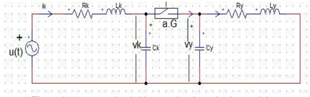
Figure 1 shows and proposes a circuit model for switching analysis for the power circuits.

Figure 1. A proposed switching transient investigation model If the switch is open a=0; a.G =0 and it means no conductivity. When the switch is closed a=1; a.G is very large, it means that circuit is closed. Source voltage is assumed pure sinus signal as U(t)=

V.sin( )

State model of the system is derived the circuit which is shown in figure1 and they are given in below,

. = - – u(t) (2.1) . = – a.G( ) (2.2)

. = (2.3) . =a.G ( ) - (2.4)

(3)

= + (2.5)

Output magnitudes of the system are mentioned in equation (2.6). Here; : Current passing through the switch and : Recovery voltage

= (2.6)

When the switch is closed a=1, a.G: Very large, = ; = In this situation both and can not be state variables at the same time. If we is chosen as a state variable equation (2.2) and 2.(4) can be written as shown below:

. = (2.7) . = (2.8) Adding equation (7) and (8) gives;

. = - (2.9) = - (2.10) For the closed switch condition, state equations become as below:

= + (2.11)

(4)

16

When the switch is closed, it can be investigated the below transient events using equation (2.11) and (2.12):

a) Energization of large inductive load: and are negligible b) Energization of large capacitive load: and are negligible. c) Short circuit current: = 0 ; , and are negligible.

From special cases a, b, and c above first or second order differential equation is obtained and analytical solution of the equation can be found. Since the circuit was operating in continuous in sinusoidal mode before the switch was closed, in the investigation of transient events when the switch is closed initial conditions is obtained as follows ( Here, : Respective angle when the switch is closed.).

= ; ; ( 2.13 )

= ( 2.14 )

= = (2.15 )

=0 ( 2.16 )

A graphical based interface is created in MATLAB environment to ease the analysis. This interface is shown in figure 2.

(5)

3. ANALYSIS OF HIGHLY INDUCTIVE LOAD

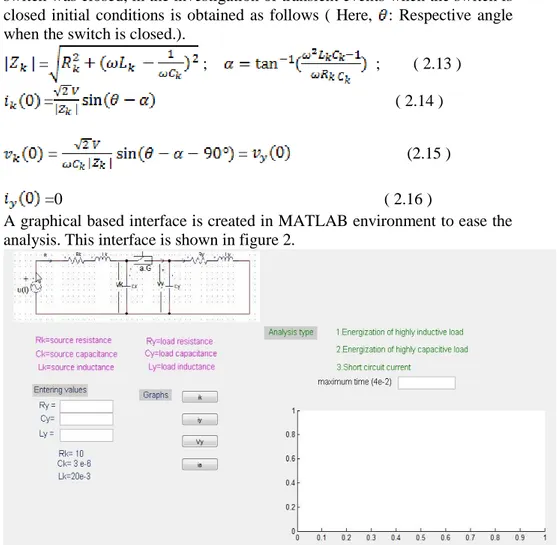
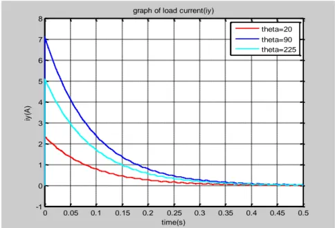
Graph of load current ( ) is again observed in three different values of . In this case load current shows a transient behavior before reaching its steady state. At the beginning the value of load current rise to a value higher than the maximum value when the steady state is reached.

Also for all values of this behavior is observed however for different values of the maximum value reached at the beginning is different (figure 3). 0 0.002 0.004 0.006 0.008 0.01 0.012 0.014 0.016 0.018 0.02 -0.03 -0.02 -0.01 0 0.01 0.02 0.03

graph of load current(iy)

time(s) iy (A ) theta=20 theta=90 theta=225

Figure 3. Load current for different values of during energization of highly inductive load.

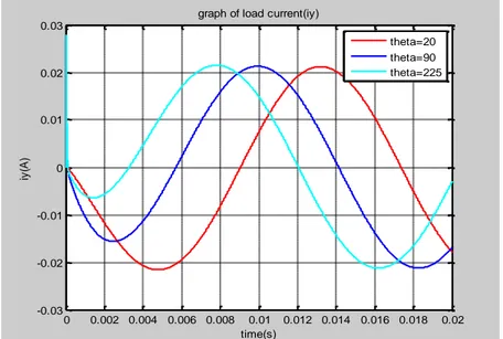
It is observed that when the value of is equal to the load current make the highest peak at the beginning compared to other values of . And figure 4 is the graph of the load current when the value of is equal to when drawn separately.

(6)

18 0 0.002 0.004 0.006 0.008 0.01 0.012 0.014 0.016 0.018 0.02 -0.03 -0.02 -0.01 0 0.01 0.02 0.03

time(s)

iy

(A

)

Figure 4. Load current during energization of highly inductive load when the value of

The initial variation of the current related to this condition is shown figure 5.

0 0.1 0.2 0.3 0.4 0.5 0.6 0.7 0.8 0.9 1 x 10-3 -0.015 -0.01 -0.005 0 0.005 0.01 0.015 0.02 0.025 0.03

time(s)

iy

(A

)

Figure 5. Load current during energization of highly inductive load when the value of zoomed at interval [0 - ].

(7)

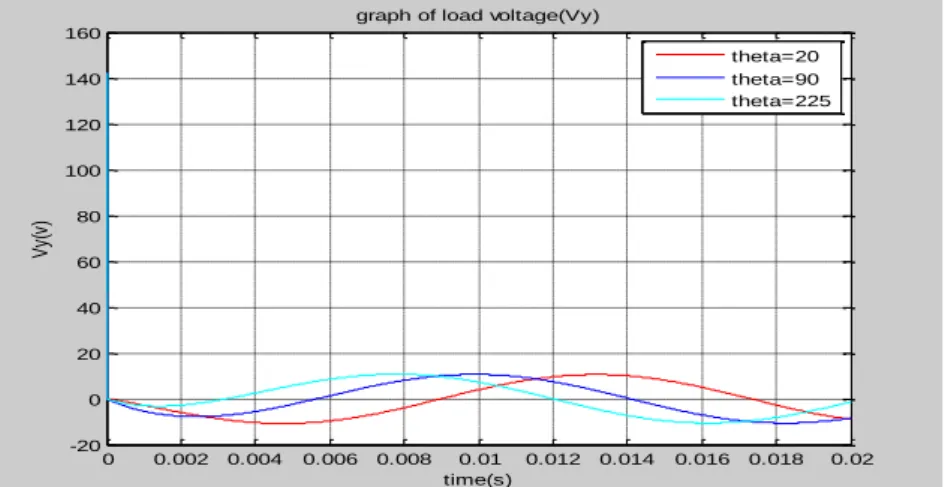
Similar to load current load voltage also shows a transient behavior at the beginning. The value of load voltage rises to a value greater than its steady state peak value. Different values of gives different values of initial peak voltage. And from observation of three value of the value has the highest initial peak value of the three. Figure 6 shows the graph of the load voltage for different values of when input peak voltage v=100V. when Load voltage during energization of highly inductive load for is zoomed in interval [0 ], peak value of the signal can be observed clearly as given figure 7.

0 0.002 0.004 0.006 0.008 0.01 0.012 0.014 0.016 0.018 0.02 -20 0 20 40 60 80 100 120 140 160

graph of load voltage(Vy)

time(s) V y( v) theta=20 theta=90 theta=225

Figure 6. graph of load voltage for different values of during energization of highly inductive load.

0 1 2 3 x 10-4 -20 0 20 40 60 80 100 120 140 160

time(s)

V

y(

v)

Figure 7. Load voltage during energization of highly inductive load for zoomed in interval [0 ].

(8)

20

4. ANALYSIS OF HIGHLY CAPACITIVE LOAD

When the capacitance of load capacitor ( ) is large, load resistance and inductance can be neglected. And the circuit acts as if it has only capacitor.

The load current shows the transient behavior before reaching its steady state, it at the time 0 the current rises to a higher value and from there is start falling slowly with sinusoidal ripples. When it reaches its steady state it continues with sinusoidal mode. Different values of makes the graph rise to the different initial values as shown in figure 8. The value rises to the highest value at the beginning and below is its graph. Continuous wave for the load current is given figure 9.

0 0.05 0.1 0.15 0.2 0.25 0.3 0.35 0.4 0.45 0.5 -1 0 1 2 3 4 5 6 7 8

time(s) iy (A ) theta=20 theta=90 theta=225

Figure 8. Graph of load current for different values of during energization of highly capacitive load.

(9)

0.645 0.65 0.655 0.66 0.665 0.67 0.675 0.68 0.685 -0.25 -0.2 -0.15 -0.1 -0.05 0 0.05 0.1 0.15 0.2 0.25

time(s)

iy

(A

)

Figure 9. Graph of load current during energization of highly capacitive load for zoomed in interval [0.6 0.7]

Unlike load current, load voltage does not start at 0V at time= 0 seconds instead it start at higher value and falls slowly to its steady state value. Different values of rises to a different value with giving the highest value of the three (figure 10). Graph of the load voltage during energization of highly capacitive load for is shown in figure 11.

0 0.05 0.1 0.15 0.2 0.25 0.3 0.35 0.4 0.45 -20 0 20 40 60 80 100 120 140

time(s) V y( v) theta=20 theta=90 theta=225

Figure 10. graph of the load voltage for different values of during energization of highly capacitive load.

(10)

22 0 0.1 0.2 0.3 0.4 0.5 0.6 -20 0 20 40 60 80 100 120 140 160

graph of load voltage(vy)

time(s)

V

y

(v

)

Figure 11. graph of the load voltage during energization of highly capacitive load for

Graph of the load voltage during energization of highly capacitive load for zoomed in interval [0.6 0.7] and it is given in figure 12.

0.65 0.655 0.66 0.665 0.67 0.675 0.68 0.685 0.69 -5 -4 -3 -2 -1 0 1 2 3 4 5

graph of load voltage(vy)

time(s)

V

y(

v)

Figure 12. graph of the load voltage during energization of highly capacitive load for zoomed in interval [0.6 0.7]

(11)

5. CONCLUSION

When the sinusoidal input is applied to the circuit, highly inductive load and highly capacitive load makes the circuit to show transient behavior before reaching its steady state. The transient behaviors are different for different types of loads. Depending on values of angle when the circuit is closed ( ), transient time can be short or long. During transient periods, overvoltage occurs most of the time. To analyze and examine this kind of overvoltage is not easy every time due to complex parameters. This study offers a simple and effective method to analyze closing transients and overvoltage which occurs because of transients.

REFERENCES

[1] J. A.Martinez-Velasco, Power System Transients, Parameter

Determination. Boca Raton, FL: CRC, Taylor & Francis Group, 2010.

[2] P. Mestas and M. C. Tavares, “Comparative analysis of control switching transient techniques in transmission lines energization maneuver,” presented at the Int. Conf. Power Syst. Transients, Lyon, France, Jun. 4–7, 2007.

[3] M. Sanaye-Pasand, M. R. Dadashzadeh, and M. Khodayar, “Limitation of transmission line switching overvoltages using switchsync relays,” presented at the Int. Conf. Power Syst. Transients, Montreal, QC, Canada, Jun. 19–23, 2005.

[4] K. M. C. Dantas,D. Jr. Fernandes, W. L. A. Neves, B. A. Souza, and L. C. A. Fonseca, “Mitigation of switching overvoltages in transmission lines via controlled switching,” presented at the IEEE Power Energy Soc. Gen. Meeting, Pittsburgh, PA, Jul. 20–24, 2008.

[5] U. Samitz, H. Siguerdidjane, F. Boudaoud, P. Bastard, J. P. Dupraz,M. Collet, J.Martin, and T. Jung, “On controlled switching of high voltage unloaded transmission lines,” in Proc. Elektrotech. Inf., Paris, France, Aug. 2002, vol. 119, no. 12, pp. 415–421.

[6] K. Frohlish, C. Hoelzl, M. Stanek, A. C. Carvalho, W. Hofbauer, P. Hoegg, B. L. Avent, D. F. Peelo, and J. H. Sawada, “Controlled closing on shunt reactor compensated transmission lines part I: Closing control device development,” IEEE Trans. Power Del., vol. 12, no. 2, pp. 734–740, Apr. 1997.