Adaptation of multiway-merge sorting algorithm to MIMD architectures with an experimental study

ADAPTATION OF MULTIWAY-MERGE SORTING

ALGORITHM TO MIMD ARCHITECTURES

WITH AN EXPERIMENTAL STUDY

A THESIS

SUBMITTED TO THE DEPARTMENT OF COMPUTER ENGINEERING AND THE INSTITUTE OF ENGINEERING AND SCIENCE

OF BILKENT UNIVERSITY

IN PARTIAL FULLFILLMENT OF THE REQUIREMENTS FOR THE DEGREE OF

MASTER OF SCIENCE

By

Levent Cantürk

April, 2002

ii

Prof. Dr. Cevdet Aykanat ( Advisor )

I certify that I have read this thesis and that in my opinion it is fully adequate, in scope and in quality, as a thesis for the degree of Master of Science.

Assoc. Prof. Dr. Özgür Ulusoy

I certify that I have read this thesis and that in my opinion it is fully adequate, in scope and in quality, as a thesis for the degree of Master of Science.

Asst. Prof. Dr. Attila Gürsoy

Approved for the Institute of Engineering and Science:

Prof. Dr. Mehmet B. Baray Director of the Institute

iii

ADAPTATION OF MULTIWAY-MERGE SORTING

ALGORITHM TO MIMD ARCHITECTURES

WITH AN EXPERIMENTAL STUDY

M.S. in Computer Engineering Supervisor: Prof. Dr. Cevdet Aykanat

April, 2002

Sorting is perhaps one of the most widely studied problems of computing. Numerous asymptotically optimal sequential algorithms have been discovered. Asymptotically optimal algorithms have been presented for varying parallel models as well. Parallel sorting algorithms have already been proposed for a variety of multiple instruction, multiple data streams (MIMD) architectures. In this thesis, we adapt the multiway-merge sorting algorithm that is originally designed for product networks, to MIMD architectures. It has good load balancing properties, modest communication needs and well performance. The multiway-merge sort algorithm requires only two all-to-all personalized communication (AAPC) and two one-to-one communications independent from the input size. In addition to evenly distributed load balancing, the algorithm requires only size of 2N/P local memory for each processor in the worst case, where N is the number of items to be sorted and P is the number of processors. We have implemented the algorithm on the PC Cluster that is established at Computer Engineering Department of Bilkent University. To compare the results we have implemented a sample sort algorithm (PSRS Parallel Sorting by Regular Sampling) by X. Liu et all and a parallel quicksort algorithm (HyperQuickSort) on the same cluster. In the experimental studies we have used three different benchmarks namely Uniformly, Gaussian, and Zero distributed inputs. Although the multiway-merge algorithm did not achieve better results than the other two, which are theoretically cost optimal algorithms, there are some cases that the multiway-merge algorithm outperforms the other two like in Zero distributed input. The results of the

iv

performance on a wide spectrum of MIMD architectures.

Keywords: Sorting, parallel sorting, algorithms, multiway-merge sorting, sorting in clusters.

v

ÇOK YÖNLÜ PARALEL BİRLEŞTİRME SIRALAMA

ALGORİTMASININ

DENEYSEL ÇALIŞMALARI İLE BİRLİKTE

ÇOKLU KOMUT ÇOKLU DATA MİMARİLERİNE

UYARLANMASI

Bilgisayar Mühendisliği, Yüksek Lisans Tez Yöneticisi: Prof. Dr. Cevdet Aykanat

Nisan, 2002

Elemanları sıralama problemi, hesaplamalarda muhtemelen üzerinde en çok çalışmış olan problemlerin başında gelmektedir. Bu konuda oldukça fazla optimum algoritmalar geliştirilmiştir. Bu algoritmalar birçok paralel model üzerinde denendi. Bunlar arasında tabi ki çoklu komut çoklu data (ÇKÇD) mimarileri için önerilen ve oldukça iyi çalışan algoritmalar da yer aldı. Bu çalışmamızda biz de, esasen ürün ağları için tasarlanmış çok yönlü birleştirme paralel sıralama algoritmasını ÇKÇD mimarilerine uygun hale getirdik. Çalışmamız, iş yükünün parallel makinalara dengeli dağıtılması, bilgisayarlar arasındaki iletişim yükünün azaltilması ve kendine has performans özellikleriyle oldukça başarılı bir uyarlamadır. Çok yönlü birleştirme sıralama algoritması, sıralanacak eleman sayısından bağımsız olarak sadece iki kere bütün bilgisayarlardan bütün bilgisayarlara kişisel iletişim ve iki kere de bilgisayardan bilgisayara iletişime ihtiyaç duymaktadır. Ek olarak, bu algoritma en kötü olasılıkla 2N/P kadar lokal belleğe ihtiyaç duymaktadır. Burada N sıralanacak eleman sayısını, P ise sıralamada kullanılacak işlemci sayısını temsil etmektedir. Algoritmayı Bilkent Üniversitesi Bilgisayar Mühendisliğinde kurulmuş olan dağıtık bellekli bilgisayar kümesi üzerinde programlayarak test ettik. Sonuçları karşılaştırma açısından bir tane örneklemeye dayalı paralel sıralama algoritmalarından (PSRS) bir

vi

kalite testi “uniformly”, “Gaussian” ve “Zero” olmak üzere uyguladık. Çok yönlü birleştirme algoritması diğer iki algoritmaya göre daha iyi sonuçlar elde etmemesine rağmen, “Zero” kalite testinde olduğu gibi bazı durumlarda da diğer algoritmaları geçmiştir. Deneylerin sonuçları raporda detaylı olarak sunulmuştur. Çok yönlü birleştirme algoritması en iyi sıralama algoritması olmamasına rağmen, bir çok ÇKÇD mimarisindeki bilgisayarda çalışabilecek ve kabul edilebilir performans verebilecek bir algoritmadır.

Anahtar sözcükler: Sıralama, paralel sıralama, algoritmalar, çokyönlü-birleştirme sıralaması, bilgisayar kümelerinde sıralama.

vii

I would like to express my special thanks and gratitude to Prof. Dr. Cevdet Aykanat, from whom I have learned a lot, due to his supervision, suggestions, and support during the past year. I would like especially thank to him for his understanding and patience in the critical moments.

I am also indebted to Assoc. Prof. Dr. Özgür Ulusoy and Assist. Prof. Dr. Attila Gürsoy for showing keen interest to the subject matter and accepting to read and review this thesis.

I would like to thank to my parents for their morale support and for many things.

I am grateful to all the honorable faculty members of the department, who actually played an important role in my life to reaching the place where I am here today.

I would like to individually thank all my colleagues and dear friends for their help and support especially to Bora Uçar and Barla Cambazloğlu.

viii

1 Introduction...1

1.1 Overview ...1

1.2 Outline of the Thesis ...2

2 Parallel Sorting...4

2.1 Motivation ...4

2.2 Parallel Architectures ...5

2.2.1 PC Clusters ...5

2.2.2 Bilkent University Beowulf PC Cluster ‘BORG’ ...6

2.3 The Sorting Problem ...8

2.4 Related Works ...8

2.4.1 Bitonic Sort Algorithm ...10

2.4.2 Odd-Even Merge Sort Algorithm ...12

2.4.3 Column Sort...14

2.4.4 Multiway-Merge Algorithm ...16

2.4.5 Parallel Sorting by Regular Sampling (PSRS) ...20

2.4.6 Hypercube Quicksort...23

3 Adaptation of Multiway-Merge Algorithm to MIMD Architectures...26

3.1 The Adapted Algorithm...26

3.2 A Complete Example ...32

3.3 Complexity Analysis ...35

3.4 Design Approach...38

4 Experimental Results and Analysis...40

4.1 Evaluating Algorithms ...40

4.1.1 Running Time ...40

4.1.2 Number of Processors...41

4.1.3 Cost...42

ix

5 Conclusion ...70 6 Appendices...79

x

2.1 The operations of steps 2 and 4 of columnsort. This figure is taken from [16]. For simplicity, this small matrix is chosen to illustrate the steps, even though its

dimensions fail to obey the Column Sort restrictions on r and s...14

2.2 The operations of steps 6 and 8 of Column Sort. This figure is taken from [16]. .15 2.3 A complete example for column sort...16

3.1 Initial unsorted N numbers distributed to P processors...27

3.2 Logical representation of step 2 for one processor, arrows ...28

3.3 Logical representation of step 3 for one processor, arrows indicate column wise reading order ...29

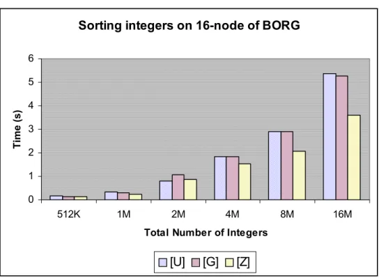
4.1 Comparison of different benchmarks, while sorting on 16 nodes of BORG with PSORT...47

4.2 Scalibility of sorting integers [U] with respect to problem size, for different numbers of processors using PSORT...48

4.3 Scalability in problem size for 16 nodes ...49

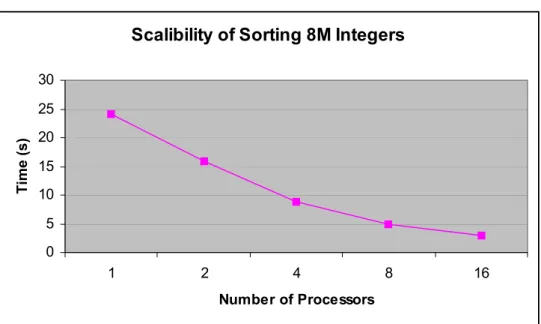
4.4 Scalibility of sorting 8M integers for different number of processors ...49

4.5 Speedup versus number of processors for different sizes of input [U]...51

4.6 Speedup versus number of processors for different sizes of input [G]...52

4.7 Speedup versus number of processors for different sizes of input [Z] ...52

4.8 Distribution of execution time by step on 16 nodes of BORG ...55

4.9 Distribution of execution time by step on 8 nodes of BORG ...55

4.10 Execution time versus number of uniformly distributed [U] inputs...60

4.11 Execution time versus number of Gaussian distributed [G] inputs ...61

4.12 Execution time versus number of zero distributed [Z] inputs ...62

4.13 Speed up versus number of uniformly distributed [U] inputs ...63

4.14 Speed up versus number of Gaussian distributed [G] inputs...64

xi

4.1 Total execution time (in seconds) for sorting 512K, 1M, 2M, 4M, 8M, 16M integers [U] with PSORT on various processors in the BORG PC cluster system. One processor data is obtained by running a sequential Quicksort algortihm on the input...45 4.2 Total execution time (in seconds) for sorting 512K, 1M, 2M, 4M, 8M, 16M

integers [G] with PSORT on various processors in the BORG PC cluster system. One processor data is obtained by running a sequential Quicksort algortihm on the input...45 4.3 Total execution time (in seconds) for sorting 512K, 1M, 2M, 4M, 8M, 16M

integers [Z] on with PSORT various processors in the BORG PC cluster system. One processor data is obtained by running a sequential Quicksort algortihm on the input...46 4.4 Speedup values of PSORT for different input [U] sizes on various number of

processors...50 4.5 Speedup values of PSORT for different input [G] sizes on various number of

processors...50 4.6 Speedup values of PSORT for different input [Z] sizes on various number of

processors...50 4.7 Efficiency of PSORT for various numbers of processors on different input [U]

sizes...53 4.8 Efficiency of PSORT for various numbers of processors on different input [G]

sizes...53 4.9 Efficiency of PSORT for various numbers of processors on different input [Z]

sizes...54 4.10 Total execution time (in seconds) for sorting 512K, 1M, 2M, 4M, 8M, 16M

integers [U] with Hyperquicksort on various processors in the BORG PC cluster system. One processor data is obtained by running a sequential Quicksort algorithm on the input...57

xii

system. One processor data is obtained by running a sequential Quicksort algorithm on the input...57 4.12 Total execution time (in seconds) for sorting 512K, 1M, 2M, 4M, 8M, 16M

integers [Z] with Hyperquicksort on various processors in the BORG PC cluster system. One processor data is obtained by running a sequential Quicksort algorithm on the input...58 4.13 Total execution time (in seconds) for sorting 512K, 1M, 2M, 4M, 8M, 16M

integers [U] with PSRS on various processors in the BORG PC cluster system. One processor data is obtained by running a sequential Quicksort algorithm on the input...58 4.14 Total execution time (in seconds) for sorting 512K, 1M, 2M, 4M, 8M, 16M

integers [G] with PSRS on various processors in the BORG PC cluster system. One processor data is obtained by running a sequential Quicksort algortihm on the input...59 4.15 Comparison of total execution times (in seconds) for sorting 512K, 1M, 2M,

4M, 8M, 16M integers [U] with PSORT, PSRS, and QSORT on various processors in the BORG PC cluster system. One processor data is obtained by running a sequential Quicksort algortihm on the input...60 4.16 Comparison of total execution times (in seconds) for sorting 512K, 1M, 2M,

4M, 8M, 16M integers [G] with PSORT, PSRS, and QSORT on various processors in the BORG PC cluster system. One processor data is obtained by running a sequential Quicksort algortihm on the input...61 4.17 Comparison of total execution times (in seconds) for sorting 512K, 1M, 2M,

4M, 8M, 16M integers [Z] with PSORT, PSRS, and QSORT on various processors in the BORG PC cluster system. One processor data is obtained by running a sequential Quicksort algortihm on the input. NA means Not Applicable ...62 4.18 Comparison of speedup values for different input [U] sizes on various number of processors for PSORT, PSRS, QSORT algorithms ...63

xiii

4.20 Comparison of speedup values for different input [Z] sizes on various number of processors for PSORT, PSRS, QSORT algorithms ...65 4.21 Comparison of efficiencies for various numbers of processors on different input [U] sizes for PSORT, PSRS, QSORT algorithms...67 4.22 Comparison of efficiencies for various numbers of processors on different input [G] sizes for PSORT, PSRS, QSORT algorithms...68 4.23 Comparison of efficiencies for various numbers of processors on different input [Z] sizes for PSORT, PSRS, QSORT algorithms ...68 6.1 Data obtained from the experiments for sorting integers [U] on BORG with

PSORT. ...79 6.2 Row data obtained from the experiments for sorting integers [G] on BORG with PSORT...80 6.3 Row data obtained by the experiments for sorting integers [Z] on BORG with

xiv PC : personal computer

SISD : single instruction single data stream SIMD : single instruction multiple data stream MISD : multiple instruction single data stream MIMD : multiple instruction multiple data stream

MSIMD : multiple- single instruction multiple data stream AAPC : all to all personalized communication

ACU : arithmetic control unit O : asymptotic big OH

N : number of elements to be sorted P : number of processors

MPI : message passing interface PVM : parallel virtual machine

BORG : 32 node distributed memory MIMD PC-cluster of Bilkent University Pi : ith processor

ai : ith eelement of a sequence

xv

σ : the time required for either injecting or receiving one word data from network.

Tcomp : computation time Tcomm : communication time

Tseq : time of the best sequential algorithm [U] : uniformly distributed data

[G] : Gaussian distributed data [Z] : zero filled data

PSRS : parallel sorting with regular sampling PSORT : multiway-merge parallel sorting algorithm QSORT : Hyperquicksort

Chapter 1

1 Introduction

1.1 Overview

This thesis is devoted to the study of one particular computational problem and the various methods proposed for solving it on a parallel computer system. The chosen problem is that of sorting a sequence of items and is widely considered as one of the most important problems in the field of computing science. This work, therefore, is about parallel sorting.

Unlike conventional computers, which have more or less similar architectures, a host of different approaches for organizing parallel computers have been proposed. For the designer of parallel algorithms (i.e., problem-solving methods for parallel computers), the diversity of parallel architectures provides a very attractive domain to work in.

PC clusters are based on a recent technology and they apply supercomputer solutions to common hardware, saving a lot of money. The task for the parallel machine is divided among the cluster nodes and the communication among processors is performed through a local network. A PC cluster is really a parallel machine and it can be programmed with the same techniques used for supercomputers. The advantage of this solution is the extreme cheapness of

hardware components: with very low cost it is possible to buy a cluster with higher performance than a workstation, i.e. paying less money.

Although there has been an increasing interest in computer clusters, there are not enough efficient parallel algorithms developed for cluster systems. Therefore adaptation of parallel algorithms for MIMD architectures like cluster systems and testing their performances appears to be an interesting problem for research. This work covers research on the new algorithms for Sorting in the lights of the new trends in parallel computing like PC clusters.

We adapted a general algorithm for the problem of sorting a sequence of items on MIMD parallel computers like PC clusters. Whatever the input size, it requires only two all-to-all-personalized communication AAPC and two point-point communications. Its expected asymptotical running time is about O( log( ))

P NP N

, where N is the number of items to be sorted and P is the number of processors used for sorting. What is more, we present and support the efficiency and scalability of multiway-merge algorithm with experimental results on a Beowulf PC cluster system. We have implemented one parallel sample sort algorithm and one parallel quicksort algorithm on the same cluster for comparing these three algorithms.

1.2 Outline of the Thesis

This work describes a parallel sorting algorithm for the problem of sorting a sequence of items on MIMD parallel computers with an experimental work on PC clusters. There have been various parallel algorithms proposed for the specific problem “sorting” on a variety of parallel architectures. The algorithms differ on the architectures where they are executed. It means that most of them depend on the special properties of the architectures on which they run.

In the second chapter of the thesis, a definition of the sorting problem is introduced. What is more, related work is given for a detailed understanding of the concepts underlying the algorithm we presented in the following chapter. In order to maintain a complete understanding edge, we briefly overviewed some important algorithms for parallel sorting. We tried to simplify the explanations of the algorithms and support with full examples.

In third chapter, our implementation of parallel sorting algorithm (which is the adaptation of multiway-merge algorithm to MIMD architectures) is described in details. A complete example is presented for a better understanding. Besides The complexity analysis of the adapted algorithm is also covered in this chapter. Lastly, a design approach, which is used in the implementation, is explained.

In the fourth chapter, the experimental results that are obtained by implementation of the algorithm on a PC cluster are reported. In addition, the important criteria for evaluating a parallel algorithm are overviewed to follow the theme presented in the chapter. A comparison of the multiway-merge algorithm with PSRS (Parallel Sorting by Regular Sampling) and Hyperquicksort is presented. The results are supported with appropriate graphics.

Chapter 2

2 Parallel Sorting

2.1 Motivation

With the growing number of areas in which computers are being used, there is an ever-increasing demand for more computing power than today’s machines can deliver. Today’s applications are required to process enormous quantities of data in reasonable amounts of time, because usage of computers is increasing dramatically in our daily life. In addition, the capacities of memories and storage devices are increased very fast. Thus, there is a need for extremely fast computers. However, it is becoming apparent that it will very soon be impossible to achieve significant increases in speed by simply using faster electronic devices, as was done in the past three decades.

Using a parallel computer is an alternative route to the attainment of very high computational speeds. In a parallel computer where there are several processing units, or processors, the problem is broken into smaller parts, each of which is solved simultaneously by a different processor. This way the solution time for a problem can be reduced dramatically by assembling hundreds or even thousands of processors. Especially when the rapidly decreasing cost of computer components is considered the attractiveness of this approach becomes more apparent.

Recently, there has been an increasing interest in computer clusters. A number of different algorithms have been described in the literature on parallel computation for sorting on MIMD computers. Therefore adaptation of parallel algorithms for MIMD architectures like cluster systems appears to be an interesting problem for research. This work covers research on the new algorithms for Sorting in the lights of the new trends in parallel computing like PC clusters.

2.2 Parallel Architectures

Using a parallel computer is an alternative route to the attainment of very high computational speeds. Unlike the case with uniprocessor computers, which generally follow the model of computation first proposed by von Neumann in the mid-1940s, several different architectures exists for parallel computers. SISD (Single Instruction Single Data), SIMD (Single Instruction Multiple Data), MISD (Multiple Instruction Single Data), MIMD (Multiple Instruction Multiple Data) are four main classifications of parallel architectures. More about parallel architectures could be found on various sources [8, 9, 11, 12, 13, 14, and 36].

In this part we will present a short introduction to the recent technology of PC (Server) Clusters and the BORG, the cluster system on which we are working.

2.2.1 PC Clusters

PC Clusters are piles of powerful PC or Alpha servers running the best available processors generally interconnected through a very high speed, low latency communication network. By working in parallel, they can provide huge amounts of computing power. Of course software has to be tuned to benefit from this architecture. Clustering technology offers by far the best price/performance ratio and can beat costly vector computers by an order of magnitude on many problem classes.

To date, supercomputer clusters can include mono or multiprocessor nodes, Intel, AMD and Alpha microprocessors, according to computing needs. High speed network can be chosen among Myrinet, SCI, Gigabit Ethernet, or simple Ethernet network, according to application and cost/performance objectives. Main features include easy-to-use administration graphical user interface, remote power on/off, remote boot of all or part of the cluster nodes, batch queuing of sequential and parallel jobs for optimal use of available power, intuitive user interface, full execution environment for MPI and OpenMP compliant parallel programs, performance monitoring tools, debuggers.

PC clusters are based on a recent technology and they apply supercomputer solutions to common hardware, saving a lot of money. The task for the parallel machine is divided among the cluster nodes and the communication among processors is performed through a local network.

A PC cluster is really a parallel machine and it can be programmed with the same techniques used for supercomputers. The advantage of this solution is the extreme cheapness of hardware components: with very low cost it is possible to buy a cluster with higher performance than a workstation, paying less money. Then a cluster is very scalable, and you can set up it with few PCs up to hundreds of nodes, building a machine comparable with medium-low parallel supercomputers. Performance being equal with supercomputers and workstations, PC clusters can reach price ratios up to 10-15 times lower.

2.2.2 Bilkent University Beowulf PC Cluster ‘BORG’

In this section, ‘BORG’ computer system is introduced. Because of increasing interest on cluster systems in Parallel Computing encouraged us to test the multiway-merge sorting algorithm on BORG. This short introduction will help better understanding and interpretation of the results in Chapter 4.

BORG, the cluster in Bilkent University, is made up of a group of personal computers interconnected by a non-blocking 100 Mbit switch. The nodes of the cluster have no monitor, neither keyboard, but they have powerful processors and good RAM memory. All PCs in the cluster are set up with Linux operative system and some standard tools for parallel programming (PVM [26] and MPI [23] libraries), also used on supercomputers.

As a base model Beowulf is applied in BORG. Beowulf is a kind of high-performance massively parallel computer built primarily out of commodity hardware components, running a free-software operating system like Linux, interconnected by a private high-speed network. It consists of a cluster of PCs or workstations dedicated to running high-performance computing tasks. The nodes in the cluster don't sit on people's desks; they are dedicated to running cluster jobs. It is usually connected to the outside world through only a single node. More information about Beowulf can be found in [25].

Specifically BORG is a Pentium-based pile-of-PCs of 32 machines, each with the following:

• GenuineIntel 400 MHz Pentium II CPU with 512KB cache size • 128 MB SDRAM

• 13 GB IDE disk

• 100 Mbit Ethernet cards

• Debian GNU/Linux woody distribution (3.0)

The experimental results in Chapter 4 were obtained by executing the algorithms on this system.

2.3 The Sorting Problem

Sorting is probably the most well studied problem in computing science due to practical and theoretical reasons. It is often said that 25-50% of all the work performed by computers consists of sorting data. The problem is also of great theoretical appeal, and its study has generated a significant amount of interesting concepts and beautiful mathematics. A formal definition is given as follows in [14]. Definition 1.1 The elements of set A are said to satisfy a linear order < if and only if

(1) for any two elements a and b of A, either a < b, a = b, or b < a; and (2) for any three elements a, b, and c of A, if a < b and b < c, then a < c. The linear order < is usually read “precedes”.

Definition 1.2 Given a sequence S = {x1, x2, …, xn} of n items on which a linear order is defined, the purpose of sorting is to arrange the elements of S into a new sequence S’ = { x1’, x2’, …, xn’} such that xi’ < xi+1’ for i = 1, 2, …, n – 1.

2.4 Related Works

Sorting is used in many applications and many of the algorithms in computer science depend on sorting. They require sorted data, since they are easier to manipulate than randomly ordered data. Simply if computer world would be thought as a world of zeros and ones, the only distinguished property of these are their orderings. Hence rearrangement of the ordering, sorting, has an important role in computer science. There are many asymptotically optimal algorithms found in this area. After parallel computing takes attention of scientists, parallelism of sorting was an interesting topic. Therefore today there are lots of parallel sorting algorithms offered for many varieties of parallel architectures [27]. Detailed information could be obtained from [14] which is a summary of the known parallel sorting algorithms proposed till 1985 and

following sections for later works. Since most of the famous sorting algorithms are well known, only the algorithms related with multiway-merge algorithm are covered in this section.

Most of the parallel sorting algorithms are based on the ideas in [2] of Batcher. The ideas in [2] form a basis even for today's works about parallel sorting. As mentioned in [1], algorithms that take the intuition from the ideas presented by Batcher applied to variety of parallel architectures like the shuffle-exchange network [30], the grid [10, 31], the cube-connected cycles [32], and the mesh of trees [33]. What is more, PSRS from [19, 20], and a series of works by D. Bader and et al [7] are considerable studies that could able to achieve the optimum algorithms. We can split these algorithms in two groups as Li and Sevick [38] did; the single–step algorithms and the multi-step algorithms. In the former one data, is moved only once between processors. PSRS [19, 20], sample sort [7, 39, 41] and parallel sorting by overpartitioning [38] could be classified in this group. Irregular communication requirements and difficulties in load balancing are disadvantages of the algorithms that fall into this group. The latter one -multi-step algorithms- may require multiple rounds of communication in order to obtain better load balancing. Bitonic sort [2], Column Sort [15, 16], SmoothSort [40], Hyperquicksort [18, 42], B-Flashsort [43], and Brent’s sort [44] fall into the second category. We have selected one sample algorithm from each group and implemented them in our cluster system BORG with MPI to compare with the multiway-merge algorithm.

In order to summarize famous algorithms in parallel sorting and to follow the work presented here much better, we reviewed related sorting algorithms in literature in the next following sections with a complete example for each. Batchers [2] Bitonic Sort and Odd-Even Merge Sort are important for the concept of parallel sorting. Leightons [15, 16] Column Sort is also crucial for understanding the Multiway-Merge Sort [1], and also for the adapted algorithm. PSRS and Hyperquicksort are covered since they are the selected algorithms for comparison.

2.4.1 Bitonic Sort Algorithm

One of the two efficient sorting algorithms of Batcher [2] is Bitonic Sorting. The algorithm sorts some special kind of sequence called bitonic sequences. A bitonic sequence [18, 1, 14] is a sequence of elements (a1, a2, …, an ) which satisfies either following properties:

( 1 ) there exists an index i, 1 ≤ i ≤ n, such that (a1, a2, …, ai ) is monotonically increasing and (ai+1, ai+2, …, an ) is monotonically decreasing, or

( 2 ) there exists a cyclic shift of indices so that (1) is satisfied, i.e. any rotation of a sequence which satisfies (1).

For instance, (2, 3, 5, 7, 9, 8, 4, 0) is a bitonic sequence, since it first increases and then decreases. On the other hand (1, 4, 8, 6, 5, 9) is not a bitonic sequence, because the last element 9 violates the property (1). (7, 8, 3, 1, 5) is also a bitonic sequence, because it is a cyclic shift of (5, 7, 8, 3, 1) which first increases and then decreases.

A monotonically increasing sequence can always be obtained from a bitonic sequence by applying recursively the bitonic split algorithm. A bitonic split is defined as the operation of splitting a bitonic sequence into two bitonic sequences. The

bitonic split algorithm is as follows.

Consider A = (a1, a2, …,an ) as a bitonic sequence such that a1 ≤ a2 ≤ …, ≤ an/2-1 and

an/2 ≥ an/2+1 ≥ …, ≥ an then the following subsequences A1 and A2 will give two

bitonic subsequences of A.

A1 = (min[a1, an/2], min[a2, an/2+1],…, min[an/2-1, an] ) and

A2 = (max[a1, an/2], max[a2, an/2+1],…, max[an/2-1, an] ).

EXAMPLE: Simulation of a merge operation on bitonic sequence of n = 16 element, that requires log216 bitonic splits.

Initial sequence: 4, 6, 8, 9, 10, 11, 14, 16, 80, 70, 60, 50, 40, 30, 20, 3 Split 1: 4, 6, 8, 9, 10, 11, 14, 3, 80, 70, 60, 50, 40, 30, 20, 16 Split 2: 4, 6, 8, 3, 10, 11, 14, 9, 40, 30, 20, 16, 80, 70, 60, 50 Split 3: 4, 3, 8, 6, 10, 9, 14, 11, 20, 16, 40, 30, 60, 50, 80, 70 Split 4: 3, 4, 6, 8, 9, 10, 11, 14, 16, 20, 30, 40, 50, 60, 70, 80

Sorting a sequence of length n elements by repeatedly merging bitonic sequences of increasing length is called bitonic sort. Since any subsequence with two elements is a bitonic sequence, the algorithm starts from the subsequences of length two, and then length of four, and goes like that. In each intermediate stage the adjacent bitonic sequences are merged in increasing and decreasing order respectively. The sequences obtained in the intermediate steps are also bitonic sequences, because concatenations of increasing and decreasing sequences are also bitonic sequences. The Bitonic Sorting Network was the first network that is capable of sorting n elements in O(log2_{n) time.}

EXAMPLE: Simulation of Bitonic Sorting on a sequence of n = 8 elements. The intermediate merges are omitted for simplicity; however the final bitonic merge is simulated in details for clarity.

X : increasing order

X: decreasing order

Initial sequence: 0, 3, 2, 6, 4, 1, 5, 7 Bitonic Merging sequences of length two: 0, 3, 2, 6, 4, 1, 5, 7 Result: 0, 3, 6, 2, 1, 4, 7, 5 Bitonic Merging sequences of length four: 0, 3, 6, 2, 1, 4, 7, 5 Result: 0, 2, 3, 6, 7, 5, 4, 1 Bitonic Merging sequences of length eight: 0, 2, 3, 6, 7, 5, 4, 1

Final merge in details: 0, 2, 3, 6, 7, 5, 4, 1

Split 1. 0, 2, 3, 1, 7, 5, 4, 6 Split 2. 0, 1, 3, 2, 4, 5, 7, 6 Split 3. 0, 1, 2, 3, 4, 5, 6, 7

Sorting algorithms based on this method are called bitonic sorters and there are many papers about generalization of bitonic sorters in the literature. [3], [4], [5], [34].

2.4.2 Odd-Even Merge Sort Algorithm

Odd-Even Merge Sort [13, 10] is one of the oldest and most famous algorithms in parallel computing. Let A be a sequence of n keys to be sorted. The odd-even merge sort algorithm [2] applies the odd-even merge algorithm repeatedly to merge two sequences at a time. Initially it forms n/2 sorted sequences of length two each. Next, it merges two sequences at a time so that at the end n/4 sorted sequences of length four each will remain. This process of merging continued until only two sequences of length n/2 each are left. Finally, these two sequences are merged. The odd-even merge algorithm can be ruled simply as follows.

Step 1. Assume we want to merge two sorted sequences A and B, where

A= a1, a2, …, an and B = b1, b2, …, bn . In the first step, two sequences are partitioned

in to two subsequences like Aodd = a1, a3, a5, …, an-1 and Aeven = a2, a4, a6, …, an.

Similarly B is partitioned into two sequences Bodd = b1, b3, b5, …, bn-1 and

Beven = b2, b4, b6, …, bn.

Step 2. Aodd and Beven are merged and Aeven and Bodd are merged recursively. Let call the results as O= o1, o2, …, on and E = e1, e2, …, en , respectively.

Step 3. Combine the sequences O and E and generate a new sequence C by taking one element from O and one element from E until all elements are exhausted. Hence C will be o1, e1, o2, e2, …, on, en .

Step 4. Finally, starting from element 2, sorting the subsequences of length two successively in C, will give the result of merging the initial sequences A and B.

Although [15] uses this algorithm, there are many variations of the odd-even merge in the literature. For example, in [17] step 2 is changed as recursively merging Aodd with Bodd and Aeven with Beven to yield corresponding results O and E. In step 4, they sort the subsequences of length two successively in C starting from the second element.

EXAMPLE: Simulation of Odd-Even Merge algorithm. Let us consider the problem of merging two sorted sequences A and B, where A = 0, 2, 3, 6, 8, 10, 12,13 and B = 1, 4, 5, 7, 9, 11, 14, 15

Step 1. Aodd = 0, 3, 8, 12 and Aeven = 2, 6, 10, 13 Bodd = 1, 5, 9, 14 and Beven = 4, 7, 11, 15

Step 2. O = 0, 3, 4, 7, 8, 11, 12, 15 and E = 1, 2, 5, 6, 9, 10, 13, 14 Step 3. C = 0, 1, 3 , 2, 4, 5, 7, 6, 8, 9, 11, 10, 12, 13, 15, 14

Step 4. C = 0, 1, 3 , 2, 4, 5, 7, 6, 8, 9, 11, 10, 12, 13, 15, 14 Result = 0, 1, 2, 3, 4, 5, 6, 7, 8, 9, 10, 11, 12, 13, 14, 15

EXAMPLE: Simulation of Odd-Even Merge Sort on a sequence of n = 8 elements. Initial sequence: 1, 3, 7, 6, 2, 0, 4, 5

forms n/2 sorted sequences of length 2: 1, 3, 6, 7, 0, 2, 4, 5 odd-even merge of successive sequences: 1, 3, 6, 7, 0, 2, 4, 5 finally merge the 2 last sequences: 0, 1, 2, 3, 4, 5, 6, 7

Like the Bitonic Sort, Odd-Even Merge Sorting Network was one of the first network that is capable of sorting n elements in O(log2n) time. Although it is one of the oldest parallel algorithms, it is still one of the most widely used and important algorithms in parallel sorting.

2.4.3 Column Sort

In this section, we review the Leightons Column Sort [15], which plays an important role in the adapted algorithm, and also in the following Multiway-merge Algorithm.

As in many algorithms, there are many variations of Column Sort in the literature. The simplest version of Column Sort presented by Leighton in [15] is a seven phase algorithm that sorts N items into column major order in an r x s matrix. Steps 1, 3, 5, and 7 are all the same: sort each column individually. The only exception is the sorting in Step 5. In Step 5, adjacent columns are sorted in reverse order, however in other steps sorting is in the same order (smallest-first) for all columns. Each of Steps 2, 4, and 6 permutes the matrix entries. In Step 2, the matrix is transposed by picking up the items in column-major order and setting them down in row-major order (preserving the r x s shape, illustrated in Figure 2.1). As Leighton stated, the reverse permutation in the Step 2 is applied, picking up items in row-major order and setting them down in column-major order. Step 6 consists of two steps of odd-even transposition sort to each row. Column Sort is always sorts N items into column-major order provided that r ≥ s2_.

Figure 2.1 The operations of Steps 2 and 4 of columnsort. This figure is taken from [16]. For simplicity, this small matrix is chosen to illustrate the steps, even though its dimensions fail to obey the Column Sort restrictions on r and s.

As in [16] and [37] one other famous version of column sort is an eight phase algorithm. Steps 1, 3, 5, 7 are similar with the previous, just sorting the columns individually in smallest-first order without any exception i.e. even in Step 5 the ordering is same. Step 2 and 4 are also same as in previous. In Step 6, each column is shifted down by r/2 positions. This shift operation empties the first r/2 entries of the leftmost column, which are filled with keys of -∞, and it creates a new column on the right, the bottommost r/2 entries of which are filled with keys of ∞. In another words, top half of each column is shifted into the bottom half of that column, and the bottom half of each column is shifted into the top half of the next column. In Step 8, the reverse permutation of Step 6 is applied. Step 6 and 8 are illustrated in Figure 2.2.

Figure 2.2 The operations of Steps 6 and 8 of Column Sort. This figure is taken from [16].

EXAMPLE: Simulation of Column Sort on a sequence of N = 8 elements with r = 4 and s = 2.

After writing the elements in r x s, 4 x2 array:

Figure 2.3 A complete example for column sort

2.4.4 Multiway-Merge Algorithm

In this section, we will present the previous related works with the topic of sorting, especially the multiway- merge sorting algorithm that in fact gives the spirit of this thesis, in [1]. 3 2 1 5 6 0 7 4 Initial array 1 0 3 2 6 4 7 5 Step 1. Sort columns

1 3 6 7 0 2 4 5 Step 2. Transpose 0 2 1 3 4 5 6 7 Step 3. Sort columns

0 4 2 5 1 6 3 7 Step 4. Transpose 0 7 1 6 2 5 3 4 Step 5. Sort columns

0 6 1 7 2 4 3 5 Step 6.1. Odd-even transp.

0 6 1 4 2 7 3 5 Step 6.2. Odd-even transp.

0 4 1 5 2 6 3 7 Step 7. Sort columns

In [1] the well known odd-even merge sorting algorithm, originally due to Batcher[2] is generalized and its application on product networks are presented. In addition, they developed a new multiway-merge algorithm that merges several sorted sequences into a single sorted sequence. By using their multiway-merge algorithm they obtained a new parallel sorting algorithm that they claimed probably the best deterministic algorithm, which can be found in terms of the low asymptotic complexity with a small constant in product networks. Therefore, adaptation of that algorithm for MIMD architectures was an interesting research. In [1], the application of the multiway-merge sorting algorithm to some special product networks is covered. Efe and Fernandez give the asymptotic analysis of the algorithm for Grid, Mesh-Connected Trees (MCT), Hypercube, Petersen Cube, Product of de Brujin, and Shuffle-Exchange Networks in [1]. For Grid and Mesh-Connected Trees they obtained a bound O (N), which is optimal. For other product networks they also obtained quite optimal asymptotical bounds.

In the sorting algorithm [1], they applied the proposed multiway-merge operation recursively to the sorted subsequences. In the paper, the multiway-merge algorithm is defined as follows.

Assume we consider to merge N sorted subsequences, Ai = (a0, a1, …, am-1), for

i = 0, 1, …, N-1, into a large sorted sequence N’.

Step 1. Initially, the algorithm requires the distribution of each sorted sequence Ai

among N sorted subsequences Bi, v, for i = 0, 1, …, N-1 and v = 0, 1, …, N-1. This is

equivalent to writing the keys of each Ai on a m/N by N array in snake order and then

reading the keys column-wise to obtain each Bi, v.

Step 2. The N subsequences Bi, v found in column v are merged into a single sorted

sequence Cv for v = 0, 1, …, N-1. This step is handled in parallel for all columns by a

m is at least N3. For the columns whose length is less than N3 like N2 a sorting algorithm is used instead of a recursive call to merge.

Step 3. The sequences Cv for v = 0, 1, …, N-1 are interleaved into a single sequence

D = (d0, d1, …, dmN -1), by reading the columns Cv’s in row-major order starting from

the top row.

Step 4. To clean the ‘dirty area’ (i.e. unsorted portion), D is divided into m/N subsequences of N2 consecutive keys each. These subsequences are called as Ez,

where z = 0, 1, …, m/N – 1. Next, these subsequences are sorted in alternate orders, that is, sequence is sorted in nondecreasing order for even z and in nonincreasing order for odd z. Then two step odd-even transposition is applied between the sorted sequences in the vertical direction. In the first transposition, the elements in the rows z and z + 1 are compared and the smallest is stored in row z, while the largest is stored in the z+1th row for even z values. The second transposition is application of the same to the odd z values. Lastly, the final subsequences Ez’s are sorted in alternate

orders as in previous one. The whole sorted sequence N’ is just concatenation of the sequences Ez’s in snake-order.

Lemma 1[1]: “When sorting an input sequence of zeros and ones, the sequence D obtained after the completion of Step 3 is sorted except for a dirty area which is never larger than N2.”

Proof of this Lemma is also presented in [1].

EXAMPLE: Simulation of multiway-merge algorithm. Assume we merge N=3 sorted subsequences , Ai = (a0, a1, …, am-1), for i = 0, 1, …, 2 and m = 9 into a large

Initial sequences: A0 = 0, 2, 5, 5, 6, 7, 8, 9, 9 A1 = 0, 2, 3, 6, 6, 7, 7, 8, 9 A2 = 1, 2, 4, 5, 6, 6, 7, 8, 9 After Step1: B0 = 0, 7, 8, 2, 6, 9, 5, 5, 9 B1 = 0, 7, 7, 2, 6, 8, 3, 6, 9 B2 = 1, 6, 7, 2, 6, 8, 4, 5, 9 After Step 2: C0 C1 C2 0 2 3 0 2 4 1 2 5 6 6 5 7 6 5 7 6 6 7 8 9 7 8 9 8 9 9 After Step 3: D : 0, 2, 3, 0, 2, 4, 1, 2, 5, 6, 6, 5, 7, 6, 5, 7, 6, 6, 7, 8, 9, 7, 8, 9, 8, 9, 9 For Step 4: E0 : 0, 2, 3, 0, 2, 4, 1, 2, 5 E1 : 6, 6, 5, 7, 6, 5, 7, 6, 6 E2 : 7, 8, 9, 7, 8, 9, 8, 9, 9 After sort alternate order

E0 : 0, 0, 1, 2, 2, 2, 3, 4, 5 E1 : 7, 7, 6, 6, 6, 6, 6, 5, 5 E2 : 7, 7, 8, 8, 8, 9, 9, 9, 9

After odd-even transitions and sort alternate order E0 : 0, 0, 1, 1, 2, 2, 3, 4, 5

E1 : 7, 7, 6, 6, 6, 6, 6, 5, 5 E2 : 7, 7, 8, 8, 8, 9, 9, 9, 9

2.4.5 Parallel Sorting by Regular Sampling (PSRS)

One of the famous algorithm among the recent parallel sample sorting algorithms is parallel sorting by regular sampling offered by X.Li et al [19, 20] in 1996. This algorithm is suitable for a diverse range of MIMD architectures. The time complexity of PSRS is asymptotic to O( n

p n

log ) when _{n≥ p}3_{, which is cost optimal [20] . It has} a good theoretical upperbound on the worst case load balancing among other sample sort algorithms. If we assume there is no duplicate keys, it has proven that in PSRS no processor has to work on more than 2n/p data elements if _{n≥ p}3_.

The algorithm consists of four phases; a sequential sort, a load balancing phase, a data exchange and a parallel merge. In order to sort n numbers (with indices 1, 2, 3, …, n) the algorithm uses p processors (1, 2, 3, …, p), so as in previous algorithms initially the data n is distributed over p processors. Basically we assume each processor has its random portion of the data already stored within them.

Phase 1. In parallel, each processor sorts their contiguous block of n/p items that is assigned to them. A sequential quicksort or merge sort can be used here. Expected runtime of the quicksort algorithm is O(nlogn), but may have a worst case of O(n2). If this is a problem, an algorithm with a worst case of O(nlogn), such as merge sort, can be used. After local sorting, processors select the samples that represent the locally sorted blocks. Here in this part, processors select the elements at local indices 1, n/p+1, 2n/p+1, …, (p-1)n/p+1, to form the samples. These p elements are called regular samples of the local elements and represent the value distribution at each processor. Therefore collection of these p elements from p processors will give the regular sample of the initial n numbers to be sorted. This process is called regular sampling load balancing heuristic.

Phase 2. This phase consists of pivot finding and local partitioning according to the pivots. In order to find pivots each processor sends the local regular samples which are potential candidates of the pivots, to a specific processor. The designated processor sorts the regular samples and selects the elements with indices p + p/2, 2p + p/2, 3p + p/2, …, (p-1) + p/2. These selected (p-1) elements forms the pivots. These pivots are distributed to each processor. Upon receiving the processors, each processor forms p partitions (s1, s2, s3, …,sp) from their sorted local blocks according

to the pivots.

Phase 3. Processors apply the total exchange algorithm for their p partitions. In other words, each processor i keeps the ith partition si itself and assigns the j

partitition sj to the jth processor. As an example, processor 3 keeps the 3rd partition

itself and gathers all the 3rd partitions of other p-1 processors, while sending its remaining partitions to the appropriate processors.

Phase 4. In this phase, each processor merges its p partitions in parallel. Since the partitions are already sorted, P-way merge algorithm will give a whole sorted sequence. After completion of phase 4, any element in processor i is greater than any element in processor j where i > j and within each processor n/p elements are sorted among themselves. So the concatenation of all local lists will give the final n element sorted list.

The implementation details and experimental results are explained in later chapters.

EXAMPLE: Simulation of PSRS on a sequence of n = 27 elements with p = 3 processors [42].

Initial unsorted sequence:

8, 23, 15, 3, 12, 22, 6, 21, 0, 9, 26, 11, 4, 20, 14, 2, 16, 24, 19, 18, 13, 7, 5, 1, 17, 25, 10

The elements are distributed to the processors evenly: P1 = 8, 23, 15, 3, 12, 22, 6, 21, 0

P2 = 9, 26, 11, 4, 20, 14, 2, 16, 24 P3 = 19, 18, 13, 7, 5, 1, 17, 25, 10

PHASE 1

Each processor sort its local elements (n/p = 27/3=9) with a sequential sorting algorithm. Then they select, in parallel, their local regular samples.

P1 = 0, 3, 6, 8, 12, 15, 21, 22, 23 Local regular samples: 0, 8, 21 P2 = 2, 4, 9, 11, 14, 16, 20, 24, 26 Local regular samples: 2, 11, 20 P3 = 1, 5, 7, 10, 13, 17, 18, 19, 25 Local regular samples: 1, 10, 18

PHASE 2

Local regular samples are gathered and sorted (p2 = 9 elements). Two (p-1) pivots are selected and distributed to the processors. Each processor generates three partitions according to the pivots.

Gathered Regular Sample: 0, 8, 21, 2, 11, 20, 1, 10, 18 Sorted Regular Sample : 0, 1, 2, 8, 10, 11, 18, 20, 21

Pivots : 8, 18

P1 = 0, 3, 6, 8, 12, 15, 21, 22, 23 P2 = 2, 4, 9, 11, 14, 16, 20, 24, 26 P3 = 1, 5, 7, 10, 13, 17, 18, 19, 25

PHASE 3

Total exchange algorithm on the partitions.

P1 = 0, 3, 6, 8, 2, 4, 1, 5, 7 P2 = 12, 15, 9, 11, 14, 16, 10, 13, 17, 18 P3 = 21, 22, 23, 20, 24, 26, 19, 25

PHASE 4

Each processor merges its new p partitions after total exchange. P1 = 0, 1, 2, 3, 4, 5, 6, 7, 8

P2 = 9, 10, 11, 12, 13, 14, 15, 16, 17, 18 P3 = 19, 20, 21, 22, 23, 24, 25, 26 Final sorted array:

0, 1, 2, 3, 4, 5, 6, 7, 8, 9, 10, 11, 12, 13, 14, 15, 16, 17, 18, 19, 20, 21, 22, 23, 24, 25, 26

2.4.6 Hypercube Quicksort

Quicksort is one of the most common sorting algorithms for sequential computers because of its simplicity, low overhead and optimal average complexity. Quicksort is often the best practical choice for sorting because its very efficient on the average that is, its expected running time is Θ(nlogn) for sorting n numbers. Although its worst case running time is Θ(n2), it also uses the advantages of inplace algorithms and performs well even in virtual memory environments. Of course, there are variety of parallel versions of such a famous algorithm in the literature [39, 46, 47, 48]. They are similar in the main idea, but differ in the architectures they run, selection of the pivots, or some parallel specific concepts like load balancing etc. In this section we present one of the parallel formulations of the quicksort algorithm [18, 42].

As it is known, Quicksort is a diviede&conquer paradigm algorithm. The simple algorithm to sort an array A[p, r] given in [45] is as follows:

Divide : The array A[p,r] is partitioned into two nonempty sub arrays A[p,q] and A[q+1, r], such that each element in the former is less than or equal to each element in the latter. The index q is computed as a part of this partitioning process.

Conquer: The two subarrays A[p, q] and A[q+1, r] are sorted recursively by calling Quicksort.

Combine: The entire array A[p, r] is sorted, since the subarrays are sorted in place, so work for combine step.

One of the basic ways of parallelizing of Quicksort is running of the recursive calls in parallel processors. Since sorting of the subarrays are two completely independent subproblems, they can be solved in parallel. Three distinct parallel formulations of Quicksort : one for a CRCW PRAM, one for a hypercube, and one for a mesh is presented in [18]. In this section, we are briefly focused on HyperQuick1 sort algorithm which we have implemented in BORG for comparison purposes. Hypercube Quicksort, as it is understood from its name, uses advantage of topological properties of a hypercube. The hyperquicksort algorithm works as follows. Let n be the number of elements to be sorted and p=2d be the number of processors in a d-dimensional hypercube. Initially we assume, as it is a convention in most algorithms in this work, the n numbers are evenly distributed to each processor. So each processor gets a block of n/p elements. At the end, elements in processor i is less than or equal to the elements in processor j where i < j. The algorithm starts by selecting a pivot element, which is broadcast to all processors. After receiving the pivot, each processor partitions its local elements into two blocks according to the pivot. All the elements smaller than the pivot are stored in one part and all the elements larger than the pivot are kept in other sub block. A d-dimensional hypercube can be decomposed into two (d-1) dimensional subcubes such that each processor in one subcube is connected a processor in other subcube. The corresponding processors could separate the subcubes according to the pivot by keeping smaller elements in one (d-1) subcube and sending the larger elements to the processors in the other subcube. Thus the processors connected along the dth communication link exchange appropriate blocks so that one retains elements smaller than the pivot and the other retains elements larger than the pivot. The proposed algorithm in [18] for this communication is, each processor with a 0 in the dth bit (the most significant bit) position of the binary representation of its processor label retains the smaller elements, and each processor with a 1 in the dth bit retains the larger elements. After

this step, each processor in the (d-1)-dimensional hypercube whose dth label bit is 0 will have elements smaller than the pivot and each processor in the other (d-1)-dimensional hypercube will have elements larger than the pivot. This procedure is performed recursively in each subcube, splitting the subcubes further. After d such splits – one along each dimension- the sequence is sorted with respect to the global ordering imposed on the processors. Finally, each processor sorts its local elements by using sequential Quicksort.

One important point in this algorithm is the selection of the pivot, because a bad selection of the pivot will yield poor performance. Since at each recursive step the elements are distributed according to the pivot, if the pivot does not split almost equally the elements, then this will result with a poor load balancing. What is more, the performance will degrade further at each recursive step. For example during the ith split partitioning a sequence among two subcubes with a bad pivot may cause the elements in one subcube more than the others (load imbalance). There are numerous ways of selecting the pivot. It can be the first element of a randomly selected processor or average of the average of the elements in the processors, or average of a randomly picked sample and etc. The important point here is whatever the method is; the pivot should divide almost equally the numbers to be sorted. A good approximation for a good pivot is selection of the medians at each processor for each subcube and then taking the average or median of them again. Thus the median for each processor will give a good approximation for the elements in that processor and collection of the medians of each processor will give a good sample space for that subcube in order to divide the elements evenly.

As stated in [18], the hypercube formulation of Quicksort is depends on the pivot selection. If pivot selection is good, then its scalability is relatively good. If the pivot selection is bad (worst case) then it has an exponential isoefficiency function. On the other hand, mesh formulation of Quicksort has an exponential isoefficiency function and is practical only for small values of p.

Chapter 3

3 Adaptation of Multiway-Merge

Algorithm to MIMD

Architectures

3.1 The Adapted Algorithm

This section develops the basic steps of the multiway-merge sorting algorithm. According to the problem definition of the sorting, the multiway-merge algorithm is expected to rearrange the sequence of keys (for the clarity, keys are assumed to be integers, but not necessarily) such that the resulting sequence follows the definition of a sorted sequence. As explained in [1] and [6], if an algorithm is able to sort any sequence of zeros and ones and based on compare-exchange operations, it can sort any items.

A sorted sequence [1] is defined as a sequence of keys (a0, a1, …, an-1) such

that a0 ≤ a1 ≤ … ≤ an-1. For clarity, let’s assume Pi denotes the ith processor and Ai

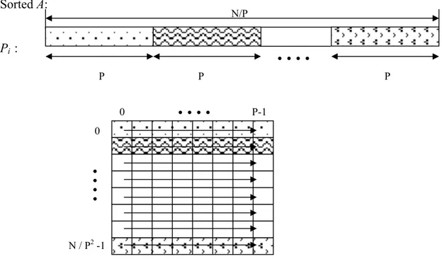
Initially we have N numbers to be sorted, and P processors available. We will assume N/P is some power of P, so each processor gets some power of Pk-1 elements where N= Pk and k > 2. Like in similar works, the number of processors P is a power of two. To start the algorithm, it is supposed that N/P numbers are distributed evenly to the processors and stored as a sequence Ai(a0, a1, …, aN/P-1) in each processor. The

output consists of the elements in non-descending order arranged amongst the processors so that the elements at each processor are in sorted order and no element at processor Pi is greater than any element at processor Pj , for all i < j.

Figure 3.1 Initial unsorted N numbers distributed to P processors

Step 1. Each P processor sorts its sequence A containing N/P numbers in parallel, using a sequential sorting algorithm like Quicksort. Here Quicksort is preferred due to its storage requirements since Quicksort is an inplace algorithm and performs very well if the whole array resides on the memory. Therefore this step requires Θ(N/P log(N/P)) expected running time. On the other hand, if memory is not a concern than usage of merge sort offers an O (N/P log(N/P)) as an upper bound for the worst case.

Step 2. Each P processor puts the sorted A containing N/P numbers into a local 2D array N/P2 by (N/P2 x P) in row-major or snake order. [1] Used snake order in the algorithm, because the orderings in snake order is more suitable for the structure of product networks. For our case, since we have two options that are

P0 : A0 PP-1 : AP-1 P1 : A1 P2 : A2 P3 : A3 • • • 0...N /P 0...N /P 0...N /P 0...N /P 0...N /P • • • P nu mb er o f pro cesso rs

feasible, in the rest of the algorithm, we preferred the row-major order. This step is illustrated in Figure 3.2 below. In the implementation of the algorithm, this should not be interpreted to imply the physical organization of data in a two dimensional array. Actually, step 2 and 3 could be handled by just rearrangement of indices of a one dimensional array.

Sorted A: Pi :

Figure 3.2 Logical representation of step 2 for one processor, arrows

indicate row-major order

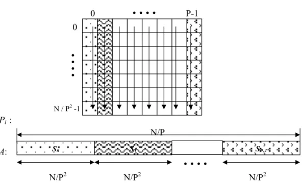
Step 3. Every processor reads its local 2D array column by column and generates P subsequences S0, S1, …, SP-1. Such that each contains N/ P2 numbers as

shown in Figure 3.3. The resulting sequences S0, S1, …, SP-1 are sorted

subsequences, since the elements within a subsequence are in the same relative order as they appeared in A which is already sorted after the result of the sorting algorithm in Step 1.

N / P2_-1 0 • • • • P-1 0 • • • • P P P • • • • N/P

Pi :

A:

Figure 3.3 Logical representation of step 3 for one processor, arrows indicate column wise reading order

Step 4. Every processor applies the total exchange (AAPC) algorithm on A with message size N/P2. That is the processors exchanges the generated subsequences S0, S1, …, SP-1 among each other in a way that Si is send to the

processor Pi. For example, processor P0 keeps S0 itself sends S1 to processor

P1, S2 to processor P2, and so on, while receiving S0 of P1 from processor P1,

S0 of P2 from processor P2, …, S0 of PN-1 from processor PN-1. The resulted

sequence A accumulated in each processor AAPC with message size m = N/ P2.

Step 5. Each processor sorts A, which is resulted from the total exchange in Step 4, using an appropriate sequential sorting algorithm. Here, P-way merge sort, where P is the number of processors, is one of the appropriate sorting algorithms, since the p subsequences S0, S1, …, SP-1 are sorted subsequences.

Or another alternative which I used in my implementation can be merging subsequences two by two for logP steps in a binary tree fashion. This step requires O(N/P logP) time.

N / P2 _-1 0 • • • • _P-1 0 • • • • N/P S0 S1 SP-1 N/P2 • • • • N/P2 N/P2

Step 6. In this step processors divide A into subsequences S0, S1, …, SP-1 of length N/

P2. That is simply Si gets the elements a_i*N/P2, a_(i*N/P2₎₊₁,..., a_i*N/P2_+N/P2₋₁. For

example, S0 gets the elements (a0, a1, …, a_N/P2₋₁), S1 gets the elements

(a_{N/ P}2,a_N/P2₊₁, …, a_2N/P2₋₁) and so on.

Step 7. Again P processors apply the total exchange (AAPC) algorithm on A with message size m = N/ P2. Therefore in this step, processors exchange their subsequences S0, S1, …, SP-1 among each other.

Step 8. Every processor sorts its N/P numbers stored in A using a sequential sorting algorithm parallel. As the same reasons with the Step 5 P-way merge sort can be used here, too.

Step 9. According to Lemma 1 in [1] we know that after Step 8, the "dirty area" (i.e. unsorted portion) is P2 length from each ends of the A. “Dirty area” is defined as the sorted subsequences within the processors whose elements may be away from their original places in the resulted sorted sequence at most P2 distance. Since every processor sorted their elements in the Step 8, only the elements at the ends of the A, may not be in the correct places for the final sorted result, because they may belong to the previous or next P2 elements. As Lemma 2 in [1] points out, if the dirty area falls into a place outside these P2 elements, then the sorting in Step 8 had to be already cleared the dirty area. This is figured out below Figure.

For one processor

P2 N / P

P2

To clear the dirty area, neighboring processors exchange the first and last P2 elements with each other while keeping their own copy, except the first and last processors. The first processor needs only to exchange its last P2 elements, and the last needs only to exchange the first P2 elements. Now, individual processors have all the potential elements that should reside on them in the result set. To make the algorithm more efficient, since we know the dirty areas are 2P2 length from ends with coming P2 elements from the neighbors, we do not need to be sort all the array. What is more, these 2P2 length subsequences are combinations of two P2 length sorted subsequences. Therefore applying merge algorithm in increasing order until obtaining the first P2 elements (just for P2 _{iterations) is enough for each processor to obtain their last P}2 _elements. On the contrary case, that is for the first P2 _{elements, applying the merge} operation in decreasing order for P2 _{iterations and getting the first P}2 _elements in the reverse order will be enough to obtain correct first P2 _{elements. So this} step requires only O(P2) time, where P is the number of processors.

Since the input is evenly distributed among the processors and the processors are assigned by almost equal amount of work at each stage of the algorithm,

load balancing of the multiway-merge algorithm is evenly distributed.

A similar approach to multiway-merge algorithm is applied for simple sorting algorithms on parallel disk systems in [17].

P2

P2 P2 P2 P2

Dirty Area Dirty Area

N / P

• • •

3.2 A Complete Example

A more sophisticated example can be obtained with N = 256 and P = 4 for observing the details in cleaning the dirty area, but for simplicity we used N = 64 numbers with P = 4 number of processors.

Initial array N = 64. Let the numbers to be sorted are:

31, 16, 3, 21, 27, 7, 6, 52, 9, 10, 11, 12, 13, 14, 15, 2, 62, 18, 40, 20, 4, 22, 23, 24, 38, 26, 5, 28, 29, 30, 1, 32, 58, 34, 35, 36, 64, 25, 59, 19, 44, 42, 43, 41, 45, 46, 47, 48, 49, 50, 51, 8, 53, 54, 55, 63, 57, 33, 39, 60, 61,17, 56, 37.

After distributing the N numbers equally to the processors, we obtain:

index 0 1 2 3 4 5 6 7 8 9 10 11 12 13 14 15 P0 : 31 16 3 21 27 7 6 52 9 10 11 12 13 14 15 2 P1 : 62 18 40 20 4 22 23 24 38 26 5 28 29 30 1 32 P2 : 58 34 35 36 64 25 59 19 44 42 43 41 45 46 47 48 P3 : 49 50 51 8 53 54 55 63 57 33 39 60 61 17 56 37

After Step 1, sorting own data:

index 0 1 2 3 4 5 6 7 8 9 10 11 12 13 14 15

P0 : 2 3 6 7 9 10 11 12 13 14 15 16 21 27 31 52

P1 : 1 4 5 18 20 22 23 24 26 28 29 30 32 38 40 62

P2 : 19 25 34 35 36 41 42 43 44 45 46 47 48 58 59 64

After Step 2, write data in 2D array: P0, P1, P2, P3, 2 3 6 7 1 4 5 18 19 25 34 35 8 17 33 37 9 10 11 12 20 22 23 24 36 41 42 43 39 49 50 51 13 14 15 16 26 28 29 30 44 45 46 47 53 54 55 56 21 27 31 52 32 38 40 62 48 58 59 64 57 60 61 63

After Step 3, read 2D array and generate P subsequences.

index 0 1 2 3 4 5 6 7 8 9 10 11 12 13 14 15

P0 : 2 9 13 21 3 10 14 27 6 11 15 31 7 12 16 52

P1 : 1 20 26 32 4 22 28 38 5 23 29 40 18 24 30 62

P2 : 19 36 44 48 25 41 45 58 34 42 46 59 35 43 47 64

P3 : 8 39 53 57 17 49 54 60 33 50 55 61 37 51 56 63

After Step 4, Total Exchange (AAPC)

index 0 1 2 3 4 5 6 7 8 9 10 11 12 13 14 15

P0 : 2 9 13 21 1 20 26 32 19 36 44 48 8 39 53 57

P1 : 3 10 14 27 4 22 28 38 25 41 45 58 17 49 54 60

P2 : 6 11 15 31 5 23 29 40 34 42 46 59 33 50 55 61

After Step 5, Sorting with successive merge operations index 0 1 2 3 4 5 6 7 8 9 10 11 12 13 14 15 P0 : 1 2 8 9 13 19 20 21 26 32 36 39 44 48 53 57 P1 : 3 4 10 14 17 22 25 27 28 38 41 45 49 54 58 60 P2 : 5 6 11 15 23 29 31 33 34 40 42 46 50 55 59 61 P3 : 7 12 16 18 24 30 35 37 43 47 51 52 56 62 63 64

After Step 6, generating subsequences

index 0 1 2 3 4 5 6 7 8 9 10 11 12 13 14 15

P0 : 1 2 8 9 13 19 20 21 26 32 36 39 44 48 53 57

P1 : 3 4 10 14 17 22 25 27 28 38 41 45 49 54 58 60

P2 : 5 6 11 15 23 29 31 33 34 40 42 46 50 55 59 61

P3 : 7 12 16 18 24 30 35 37 43 47 51 52 56 62 63 64

After Step 7, Total Exchange (AAPC)

index 0 1 2 3 4 5 6 7 8 9 10 11 12 13 14 15

P0 : 1 2 8 9 3 4 10 14 5 6 11 15 7 12 16 18

P1 : 13 19 20 21 17 22 25 27 23 29 31 33 24 30 35 37

P2 : 26 32 36 39 28 38 41 45 34 40 42 46 43 47 51 52