Breakpoint refinement of genomic structural variation using split read analysis

BREAKPOINT REFINEMENT OF GENOMIC

STRUCTURAL VARIATION USING SPLIT

READ ANALYSIS

a thesis submitted to

the graduate school of engineering and science

of bilkent university

in partial fulfillment of the requirements for

the degree of

master of science

in

computer engineering

By

Balanur ˙I¸cen

September 2019

Breakpoint Refinement of Genomic Structural Variation Using Split Read Analysis

By Balanur ˙I¸cen September 2019

We certify that we have read this thesis and that in our opinion it is fully adequate, in scope and in quality, as a thesis for the degree of Master of Science.

Can Alkan (Advisor)

C¸ i˘gdem G¨und¨uz Demir

Aybar Can Acar

Approved for the Graduate School of Engineering and Science:

ABSTRACT

BREAKPOINT REFINEMENT OF GENOMIC

STRUCTURAL VARIATION USING SPLIT READ

ANALYSIS

Balanur ˙I¸cen

M.S. in Computer Engineering Advisor: Can Alkan

September 2019

Genomic variations that vary from single nucleotide polymorphisms (SNPs), small INDELs to structural variations (SVs) are discovered to have significant pheno-typic effects on individuals. Among these genomic variations, SVs are changes that affect more than 50 nucleotides of DNA. SVs are linked to the sources of many genetic diseases such as autism, schizophrenia and chronic myelogenous leukemia. Accurate and precise characterization of these structural variants not only enables us to diagnose genetic diseases that are previously correlated with them but also it provides more reliable information to pursue higher levels of research in the genomic research pipelines. There are many SV detection tools that aim to find the approximate locations of SVs in genome, a further step in the pipeline is to refine those breakpoints of variants by a closer and more fo-cused examination. By this means, genotyping step of structural variations would be faster using k-mer based alignment-free methods and more accurate since locations of SVs will be known with 15 base pair resolution compared to 300 -500 base pair long confidence intervals. Moreover, further steps in the genomic pipelines based on the results of SV detection algorithms would have more definite data to build up on. In this thesis, we propose BROSV (Breakpoint Refinement of Structural Variation), a breakpoint refinement algorithm to obtain better res-olution on SV breakpoints with split read analysis and local assembly methods using Illumina short reads and BWA alignment tool. Implementation is available at https://github.com/BilkentCompGen/brosv.

¨

OZET

AYRIK OKUMA Y ¨

ONTEM˙I ˙ILE YAPISAL

VARYASYONLARIN KOPMA NOKTALARININ

RAF˙INE ED˙ILMES˙I

Balanur ˙I¸cen

Bilgisayar M¨uhendisli˘gi, Y¨uksek Lisans Tez Danı¸smanı: Can Alkan

September 2019

Yapılan ara¸stırmalarda tek n¨ukleotid polimorfizmi (TNP), baz ¸cifti ek-leme/¸cıkarmaları (indel) ve yapısal varyasyonlardan (YV) olu¸san genetik varyasy-onların bireylerde bir¸cok fenotipik etkileri oldu˘gu g¨ozlemlenmi¸stir. Bu genetik varyasyonlar arasından 50 n¨ukleotid ve daha fazlasını etkileyenler YV olarak ad-landırılır. YV’ler otizm, ¸sizofreni ve miyeloid l¨osemi gibi bir¸cok kalıtsal hastalı˘ga yol a¸cmaktadır. Bu varyasyonların do˘gru ve hassas bir ¸sekilde karakterize edilmesi sebep oldukları hastalıkların te¸shisine olanak sa˘glarken aynı zamanda genomik ara¸stırmaların daha ¨ust seviyede yapılması i¸cin g¨uvenilir bilgi sa˘glar. YV’lerin genomdaki yakla¸sık yerini bulmayı ama¸clayan bir¸cok YV tespit algoritması bulun-maktadır. Genomik ara¸stırmalardaki bir sonraki adım daha odaklı ve yakından bir incelemeyle YV’lerin kopma (ba¸slangı¸c/biti¸s) noktalarının rafine edilmesidir. Yakla¸sık 300 - 500 baz ¸cifti uzunlu˘gunda g¨uven aralıkları yerine kopma nokta-ları 1 - 5 baz ¸cifti ¸c¨oz¨un¨url¨ukte bilindi˘ginde, YV’lerin genotipleme a¸saması ¸cok daha hızlı ve hatasız olacaktır. B¨oylece YV tespit algoritmalarının sonu¸clarını baz alan genomik ara¸stırmaların daha sonraki a¸samaları da ¸calı¸smalarını daha kesin ve g¨uvenilir bir veri ile s¨urd¨urebileceklerdir. Bu tezde, kısa okuma teknolo-jisi ve ayrık okuma y¨ontemini kullanarak YV kopma noktası rafine eden BROSV algoritmasını sunuyoruz.

Anahtar s¨ozc¨ukler : Yapısal varyasyon, kopma noktası rafine edilmesi, ayrık okuma.

Acknowledgement

First and foremost, I would like to express my sincere gratitude to my supervisor Asst. Prof. Can Alkan, who has guided me through my graduate studies. The work presented in this thesis is only possible with his support, patience, under-standing and extensive knowledge. Aside from my advisor, I would like to thank my thesis committee: Assist. Prof. C¸ i˘gdem G¨und¨uz Demir and Assist. Prof. Aybar Can Acar for their time and consideration.

I would like to thank T ¨UB˙ITAK for financially supporting this project (T ¨UB˙ITAK Project 215E172).

I would like to thank my office mates from EA 507, especially Z¨ulal Bing¨ol for their support, encouragement and all the coffee. They made my time in the office enjoyable. I would also like to thank all members of Bilkent Bioinformatics and Computational Genomics Group, especially Ezgi Ebren and Arda S¨oylev for answering my questions and helping me along the way whenever I needed. I am also grateful for my friends Nurdan Tatar and Zeynep Ate¸s for always being on my side during this process.

I would like to express my deepest gratitude to my aikido teacher Tayfun Evyapan. He encouraged me to confront myself and helped me to grow physically, mentally and spiritually. I am thankful for all of my friends I know through aikido; especially Efekan K¨okc¨u, Mustafa C¸ olak, ˙Irem Han and Sarp Ba¸saraner. They always inspire me and with their company Bilkent felt like home.

I must express my inmost gratitude to my fianc´e, Halil, for supporting me with his never ending love and patience. He always brings me up when I feel down and keeps me going when I’m doubtful.

Finally, I owe the greatest of gratitude to my parents M¨ucahide and Hasan and my loving grandmother Hayriye for their unconditional love and support.

Contents

1 Introduction 1

1.1 Background . . . 2

1.1.1 Sequencing . . . 2

1.1.2 Sanger Sequencing . . . 2

1.1.3 Human Genome Project . . . 3

1.1.4 High Throughput Sequencing . . . 3

1.1.5 Short Read Sequencing . . . 4

1.1.6 Read Mapping . . . 4

1.1.7 Structural Variation . . . 5

1.1.8 Sequence Signatures for SV Detection Methods . . . 5

1.1.9 State-of-the-art SV discovery tools . . . 10

2 BROSV Algorithm to Refine Breakpoint of SVs using Split Read

CONTENTS vii

2.1 Motivation . . . 13

2.2 Challenge . . . 14

2.3 Mapped short read data . . . 15

2.4 Predicted SV records . . . 15

2.5 Processing alignments and predicted SV records . . . 16

2.5.1 Determining read fragment size . . . 16

2.5.2 Extracting confidence intervals for SV breakpoints . . . 16

2.5.3 Extracting signaling reads in confidence intervals . . . 17

2.6 Assembly of Signaling Reads . . . 19

2.7 Breakpoint loci from split alignments . . . 19

2.8 Majority voting on candidate locations . . . 20

3 Results 24 3.1 Simulated Data . . . 24

4 Discussion and Future Work 34 4.1 Local Assembly for Refinement . . . 34

4.2 Multiple Sequence Alignment . . . 35

4.3 Local Assembly for Novel Insertions . . . 35

CONTENTS viii

4.5 Genotyping . . . 36

4.6 Application to Real Datasets . . . 37

A Glossary 46

List of Figures

1.1 Read pair signatures for different types of SV. Adapted from [1]. . 7

1.2 Split read signatures for different types of SV. Adapted from [1]. . 9

1.3 NovelSeq, local assembly based SV detection tool. Adapted from [2]. . . 10

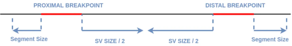
2.1 Confidence intervals are extended by segment size to left and right at proximal and distal breakpoints respectively to cover other ends of signaling discordant read pairs. They are also extended by half of the variant size inwards to cover the entire SV region. . . 17

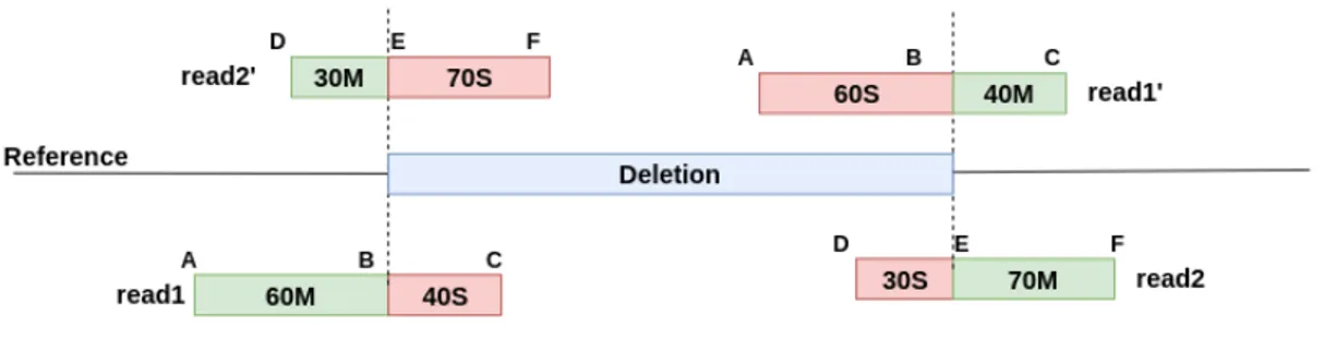
2.2 Calculation of breakpoint location from clipped alignments for deletions and inversions. Each soft/hard clipped read in a con-fidence interval signals an SV breakpoint. Indicated breakpoint location can be calculated as the position where clipped region ends and matched region starts. If clipped region comes first, indi-cated breakpoint location is the start position of alignment. Oth-erwise, ie. matched region comes first, indicated location is length of matched sequence forward from start of the alignment. . . 21

LIST OF FIGURES x

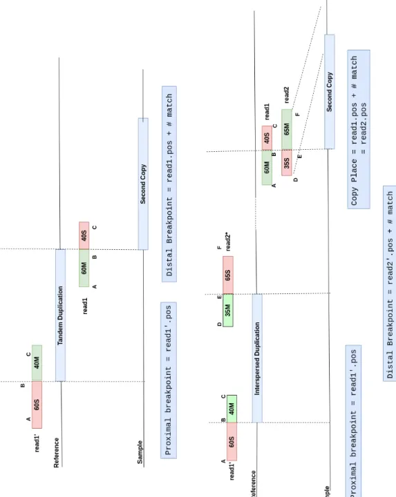
2.3 Calculation of breakpoint location from clipped alignments for du-plications. While read 1 and read 2 represents the one split align-ment of those reads, other split alignalign-ment of that reads are indi-cated as read 1’ and read 2’. Original locations of reads are shown projections at the sample genome. . . 22

2.4 Clustering and majority voting of candidate breakpoint locations. We extract signaling split reads from extended SV confidence in-tervals. Each split read signals to a candidate breakpoint location that is calculated from its CIGAR string. Then, within each clus-ter, we vote candidate locations by the reads supporting to it. Finally, we predict candidate location with the highest support as the final breakpoint. . . 23

3.1 Size distribution of confidence intervals of proximal breakpoints. Y axis shows the confidence interval size of each TARDIS prediction. X axis corresponds the final refinement result of BROSV for each prediction. . . 30

3.2 Size distribution of confidence intervals of distal breakpoints. Y axis shows the confidence interval size of each TARDIS prediction. X axis corresponds the final refinement result of BROSV for each prediction. . . 31

3.3 Number of deletion breakpoints refined by using top ranked and second ranked candidate location in majority voting. . . 32

3.4 Number of inversion breakpoints refined by using top ranked and second ranked candidate location in majority voting. . . 32

List of Tables

1.1 Read pair signatures and corresponding SV types. For duplications insert size depends on the distance between copies. For inversions insert size depends on the variant size. All read pair signatures

can signal a translocation depending on insert size. . . 7

3.1 Size distribution of variants in simulated data for each SV type. . 25

3.2 Refinement performance of BROSV for deletions using simulated data. . . 26

3.3 Refinement performance of BROSV for inversions using simulated data. . . 26

3.4 Refinement performance of BROSV for tandem duplications using simulated data. . . 27

3.5 Refinement performance of BROSV for interspersed duplications using simulated data. . . 27

3.6 Overall performance of BROSV for TARDIS predictions. . . 28

3.7 Overall performance of BROSV for DELLY predictions. . . 28

LIST OF TABLES xii

3.9 Precision, recall and F1 scores of BROSV on simulated data. . . . 29

3.10 Example tie cases in majority voting. In voting step, some can-didate locations get similar high split read support. Each row represents a candidate location for an SV breakpoint. While first row represents the top ranked location, second row represents the second ranked candidate location etc. True location for each ex-ample SV breakpoint is shown in bold. BROSV selects top ranked candidate location in our current setting. Although in these cases, actually second ranked locations reflect the true genomic loci of the breakpoint. . . 33

Chapter 1

Introduction

Genome is the hereditary material in a living organism, a complete set of its DNA. For humans, size of the whole genome is 3 billion base pairs organized in 22 autosomal chromosome pairs and two sex chromosomes, 46 chromosomes in total. Each DNA sequence consists of a permutation of 4 bases; Adenine (A), Thymine (T), Guanine (G), and Cytosine (C). 99.9% of genomic material is shared among humans. Remaining 0.1% differentiates individuals from each other [3]. These differences can be in different sizes and shapes. SNPs (single nucleotide polymorphism) is a change that affects only one base pair. Indels are deletions or insertions that affect less than 50 base pairs. These two categories of variants are more common in the genome and relatively easier to detect. Structural variations (SV) are changes in the DNA that are longer than 50 base pairs [1]. SVs can be copy number variations; deletions, insertions, duplications or they can be balanced rearrangements; inversions and translocations [4]. Some SVs are known to be the cause of genetic diseases like autism, schizophrenia, obesity, bipolar disorder and cancer [5, 6, 7, 8, 9, 10]. While SV discovery is important for genomic research pipelines, it has many difficulties due to repeats in the human genome, limitations of sequencing and read mapping technologies [11, 4, 12]. There are different approaches for SV discovery each one having different advantages and limitations (See Subsection 1.1.5 for details). In this thesis, we present BROSV a breakpoint refinement tool for imprecise SVs using split read analysis. First, we

provide detailed background information about stages of SV discovery pipeline, different SV discovery methods and some related tools to understand the need and significance of BROSV.

1.1

Background

1.1.1

Sequencing

Sequencing is the task to identify the order of the bases that forms a DNA molecule. These bases are adenine (A), thymine (T), cytosine (C), guanine (G) and they are the chemical building blocks of the genome. Sequencing turns a DNA molecule into a string that is a permutation of these 4 letters. This string is used to study whether a DNA sequence contains a gene, regulatory information or a change that could cause a disease. There is no available technology to read a chromosome from start to end. There are several methods for DNA sequencing and all sequencers have limitations in terms of read length, error rate, speed and cost. Earliest approaches for sequencing are Gilbert [13] and Sanger [14] meth-ods. Sanger sequencing is based on chain termination method and was used by the Human Genome Project. It produces long fragments (1000 base pairs) with high accuracy but it is slow and expensive. High throughput sequencing (HTS) [15] is the current sequencing method that is widely used for genomic pipelines because it provides high throughput and speed at a much cheaper cost. These methods are described in the following sections with more detail.

1.1.2

Sanger Sequencing

Sanger sequencing is regarded as the first successful application of genomic se-quencing. It had been the most popular tool for 40 years until the arrival of Illumina, second generation sequencers. It is based on chain termination method where while DNA polymerase replicates a DNA strand, a dideoxy nucleotide

(ddNTP), a nucleotide lacking a 3’ hydroxyl group, joins instead of a dNTP (deoxynucleotide), and terminates the reaction. Then, the molecules ending with ddNTPs with different lengths are sorted with capillary gel electrophoresis. Since starting point of each molecule is same, fluorescent tag on each ddNTP can iden-tify the bases in the nucleotides by their order [14, 16]. Sanger sequencing re-mained relevant for sometime since it produces DNA reads longer than 1000 nucleotides with low error rate. However, it is still more expensive and time con-suming for whole genome sequencing projects than second generation sequencing tools like Illumina. Yet, it is still valid for smaller projects and verification of results obtained by new sequencing technologies.

1.1.3

Human Genome Project

The Human Genome Project (HGP) was a multinational research project to identify, sequence and map all the genes in the human genome. HGP was led by a group of international scientists and took 14 years and cost around 3 billion dollars [17, 18]. The HGP has discovered around 20,500 human genes and provided us with a detailed source to study the structure, organization and function of human genes. It used Sanger sequencing method and DNA of 7-8 individuals to create a consensus. Reference human genome spans 99% of the DNA with >99% accuracy and it is updated regularly by adding genomes of other individuals for major alleles and resolving repeat and gap regions. Most recent version of reference genome at the time of this thesis is GRCh38 and released in 2013.

1.1.4

High Throughput Sequencing

High throughput sequencing (HTS) also referred as next generation sequencing, is a term to describe a set of different modern sequencing methods such as Illumina, Roche 454, and Ion Torrent. They allow thousands to millions of sequencing re-actions to run at once in parallel compared to Sanger sequencing which is limited in throughput [15]. This is the most important and common feature of HTS

platforms. They are also faster and cheaper than traditional methods. Due to the parallel nature of the technique, HTS platforms generate larger datasets and provide a more comprehensive insight for genomics studies [19]. Since the Human Genome Project, the cost of sequencing a human genome decreased drastically. While Whole-Genome Sequencing (WGS) with Sanger sequencing costs a few mil-lion dollars, sequencing a person’s genome with an Illumina NovaSeq costs around $1000 and takes 2 days. This improvement provides us with the opportunity of more rapid and affordable results.

1.1.5

Short Read Sequencing

Raw sequence that comes out of a sequencing machine is called a read [20]. HTS platforms like Illumina produce short reads that are 100 - 150 nucleotides long. A test donor DNA is shredded into small fragments and selected by a preset size. These fragments are copied by polymerase chain reaction (PCR) when the amount of input DNA is low. By attaching fluorescently marked bases to the fragment from both ends with DNA polymerase, bases in the sequence are determined since each type of base beams a different light. This technique can sequence until 150 base pairs before its quality degrades. Illumina platform provides reads with low error rate and it is rather cheap. Downside of studies that uses short read technology is that they are insufficient to resolve ambiguities in repeat and complex SV regions of the genome [21, 22].

1.1.6

Read Mapping

Read mapping or alignment is the first step of many bioinformatic pipelines and most common process applied on HTS data. The aim is to find the correct ge-nomic location of relatively short DNA sequences (reads) in the reference genome. Read mapping problem has several difficulties. First of all, the human genome is very repetitive, 50% of the genome consists of repeats [21]. So, determining which copy of the repeat the read originated from is not possible. Also, due to

sequencing errors, SNPs and indels that possibly occur in reads, alignments will have mismatches, complicating the process even more [23]. Lastly, since there are millions to billions of reads in HTS data, memory and time requirement is high. Hence, finding an optimal alignment using Smith-Waterman local alignment al-gorithm is not feasible, several heuristics are adopted by read mapping tools. One approach is hash based seed and extend algorithms such as mrFAST [24], mrsFAST [25], FASTHash [26], NovoAlign [27]. Another and a faster approach is based on Burrows-Wheeler Transform and Ferragina-Manzini Index based al-gorithms like Bowtie [23], Bowtie2 [28], BWA [29].

1.1.7

Structural Variation

Genomic structural variations (SVs) are the changes in the DNA that affect more than 50 base pairs. SVs come in many different flavors, such as copy number vari-ants; deletions, duplications, insertions, or balanced rearrangements; inversions and translocations. While copy number variants changes the amount of the DNA, balanced rearrangements only affect the organization of the genome. Structural variations that affect only one chromosome are called intrachromosomal events; otherwise they are called interchromosomal events that affect a pair of chromo-somes. Duplications and translocations can be interchromosomal events.

1.1.8

Sequence Signatures for SV Detection Methods

In order to detect structural variations, ideally we need one test DNA (the donor) and the reference DNA without any variation (ground truth). The aim is to find the differences (SVs) of the donor DNA from the reference. By comparing these two fully assembled genomes, SVs would be revealed. However, we only have the correctly assembled reference genome (¿99% accuracy). Due to the limitations of the current technologies, we have millions to billions of reads for the donor instead of an assembled one piece DNA. Therefore, we depend on the sequence signatures, irregular cases when reads are aligned to the reference, to discover

SVs. Insert size is the distance between the two ends of a paired end read and we mainly utilize this information in sequence signatures for SV detection. In the following section 4 main signatures; read pair, read depth, split read and assembly are explained in detail. All these signatures are based on read mapping task where billions of reads are aligned to the reference genome. irregularities in read alignment are utilized to detect SVs.

1.1.8.1 Read Pair

Read pair analysis used on the paired end sequencing data where ends of a frag-ment map to opposite strands of the DNA. Normally, one end of the fragfrag-ment maps to forward strand while the other one maps to the reverse strand within an expected insert size, length of the DNA fragment read pair originated from. These reads are called concordant reads. On the other hand, in SV regions of the genome, reads map to reference genome discordantly. There are different classes of discordant reads (See Figure 1.1). If only one end of the fragment is mapped to the reference, it is called one end anchored read (OEA). Ends of a discordant fragment can map in wrong orientation such as +/+, −/− or −/+ where + rep-resents forward, − reprep-resents reverse strand. If the ends of a fragment maps to the reference farther or closer than expected, read pair is also called discordant. All these signatures indicate the existence of a different type of variant. Table 1.1 shows the meanings of different read pair signatures.

Read pair analysis can predict deletions, insertions, inversions and duplica-tions. Size and breakpoint resolution of its predictions are bounded by insert size of the data used. There are many SV callers that utilize read pair signature such as BreakDancer [30], GenomeSTRiP [31], VariationHunter [32], HYDRA [33] and so on.

Figure 1.1: Read pair signatures for different types of SV. Adapted from [1].

Table 1.1: Read pair signatures and corresponding SV types. For duplications insert size depends on the distance between copies. For inversions insert size depends on the variant size. All read pair signatures can signal a translocation depending on insert size.

Mapping Strands Insert Size Variants

+ − > µ + 3σ Deletion, Interspersed Duplication < µ − 3σ Insertion

+ +

See above Inverted Duplication, Inversion − −

1.1.8.2 Read Depth

Read depth is a simple method used to detect copy number variants. Read depth or coverage is calculated by counting the number of reads that is mapped to a specific location in the genome. Read depth method uses irregularities in this information to predict variants. It assumes a Poisson (random) distribution for read depth. In reality, depth is biases against the regions with high or low GC density since these regions are less likely to get sequenced. This issue is addressed and corrected statistically in several detection tools using read depth analysis [24, 34]. If read depth is less than expected value (µ − 3σ) at a region, it indicates the existence of a deletion. Similarly, if read depth is greater than expected value, this signals a duplication. While this analysis is used to detect copy number variants and confirm predictions made by other SV detection techniques, it has its shortcomings. For example; in complex regions of the genome, read depth signals are not reliable due to mapping ambiguity. Also when standard deviation is high, it is hard to differentiate homozygous variants from heterozygous ones. mrCaNaVaR [35], SegSeq [36], CNVnator [34], and RDXplorer [37] are some CNV callers that employ read depth analysis.

1.1.8.3 Split Read

Split read analysis uses reads that map to variant breakpoints. When a read is originated from an SV breakpoint, part of the read maps normally and remaining section, clipped part, maps to a different location depending on the SV type. For example, clipped part maps further away for deletions, it maps closer for inser-tions, maps to reverse strand for inversions and so on (See Figure 1.2). Split read method is generally used with long reads to detect variants. It is not very suitable for short read technologies, since shorter sequence length increases map-ping ambiguity. Pindel [38], SRiC [39] and SPLITREAD [40] are SV detection tools based on split read analysis. However, split read method is usually used in combination with other signatures for SV discovery. It is also useful to refine SV breakpoints.

Figure 1.2: Split read signatures for different types of SV. Adapted from [1].

1.1.8.4 Assembly

Sequence assembly is the task of aligning and combining the smaller pieces of DNA to reconstruct the original, longer DNA sequence. Longer sequences are better at resolving ambiguous regions of the genome and offer higher chance of detecting SVs, since they can cover sequences supporting both ends of SVs, making alignment task easier to in complex regions. However, it is not a trivial task to apply at a genome-wide scale due to its computational complexity and significant memory requirements. Instead, local assembly can be a good trade-off to detect SVs by using reads originally aligned to a mutual location of interest for assembly. This targeted approach reduces computational requirements of the problem and increases the usability of the assembly method. Some of the tools that utilizes sequence assembly for SV detection are Pamir [41], PopIns [42], NovelSeq [2] and SvABA [43].

Figure 1.3: NovelSeq, local assembly based SV detection tool. Adapted from [2].

1.1.9

State-of-the-art SV discovery tools

SvABA is a tool for structural variation analysis by using local assembly. It performs local assembly on reads that deviates from reference genome to get con-sensus contigs. It forms discordant read clusters based on their possible alignment loci. Each cluster is assembled using String Graph Assembler (SGA) [44]. Then, the assembled contigs are realigns to reference using BWA-MEM to detect vari-ants. While gapped alignments produces candidate indels, contigs with multipart alignments indicate potential SVs. While SvABA exhibits high sensitivity and accuracy for indels and SVs from various sizes, its performance relies heavily on high coverage data, ie. there should be sufficient reads around a variant to build an accurate assembly [43].

novoBreak also uses local assembly for SV breakpoint detection. It is based on genome-wide classification and filtering strategy to find novo k-mers, k-mers having novel information on variant region [45]. After finding novo k-mers, it

clusters reads having the same set of novo k-mers. Each cluster is assembled into contigs using SSAKE [46]. These contigs are aligned to reference to infer breakpoints and associated variants. Most important improvement novoBreak offers over other approaches is the k-mer identification and classification strategy because it reduces the number of reported SV breakpoints and uses computational power on the more likely candidate SVs.

DELLY utilizes read pair and split read signatures to detect SVs. It clusters paired-end reads using an undirected graph. Each read pair is represented as a node. Nodes (read pairs) signaling the same SV has an edge between them. Difference between predicted variant sizes is represented as edge weights. In this setting, DELLY assume each SV is a fully connected component in the graph and it employs maximum clique heuristics to cluster the graph. Later, it uses this clusters (predicted SVs) and split read analysis to get a better breakpoint resolution [47]. While DELLY achieves high precision, it can not sustain its performance for larger variants. Moreover, it does not characterize interspersed duplication.

LUMPY is a probabilistic SV discovery tool that employs read pair and split read signatures concurrently. It transforms these alignment signals into probabilistic distribution that reflect the irregularity of a location in the genome, possibility of being a breakpoint [48]. Even though it shows high precision, it has lower sensitivity for long variants compared to other tools. And it is not able to detect interspersed duplications.

TARDIS is a SV discovery tool that utilizes read pair, read depth and split read signatures. It applies maximum parsimony problem on SV discovery in a fact that it tries to minimize the number of reported variants indicated by given discordant and split read set [49, 50]. Similar to various discovery tools TARDIS forms valid clusters using discordant read pairs and split reads until no additional read pair can be added without violating its validity [51]. Then, it uses read depth information to assign weights to clusters and eliminate likely false positive signals. TARDIS achieves better specificity and comparable sensitivity to state of the art discovery tools. It reports confidence intervals 300 - 500 base

pair long for large SVs. With BROSV, we aim to improve breakpoint resolution of tools like TARDIS. As proof-of-concept, we use TARDIS input/output data for our experiments. BROSV can be incorporated with another SV discovery tool to refine breakpoints and detect false positives signals.

Chapter 2

BROSV Algorithm to Refine

Breakpoint of SVs using Split

Read Analysis

2.1

Motivation

Connection between genomic variants and genetic diseases have been discovered by several studies. For example, duplication 17p11.2 causes Potocki-Lupski Syn-drome that results in developmental delay, heart defects, dental and skeletal ab-normalities in infants [52, 53]. Deletion of same region lead to Smith-Magenis Syndrome that causes intellectual disability, delayed language skills, distinctive facial features [54]. Williams Syndrome is caused by deletion of several genes from chromosome 7 including CLIP2, ELN, and LIMK1 [55]. This condition is characterized by mild to moderate intellectual disability or learning prob-lems, unique personality characteristics, distinctive facial features, and heart and blood vessel (cardiovascular) problems. Furthermore, there are studies that sup-port SV causaion of autism, schizophrenia, obesity, bipolar disorder and cancer [5, 6, 7, 8, 9, 10]. Therefore, precise and accurate characterization of structural variants can widen our understanding on many genetic diseases and enable us

to develop personalized treatments. Since the start of the 1000 Genome Project (1000 GP) [56], plenty of tools are developed to characterize variants thanks to newly available HTS data. For example, 19 different algorithms were developed and used in the pilot phase of the 1000 GP [57]. HTS technology provided re-searchers with the opportunity of rapid development because it has considerably low cost and time requirement compared to earlier technologies such as array CGH, SNP microarrays and Sanger sequencing. Despite there are several SV dis-covery algorithms assisting us to understand genetic disorders, there is still a need for better and detailed annotation of SVs. Since most of the tools offer imprecise SV predictions providing only confidence intervals for variant location, a bet-ter resolution would help in the validation and genotyping steps of the pipeline. BROSV offers a closer look into SVs with a targeted split read analysis.

2.2

Challenge

Exact discovery of variant breakpoints is not a trivial task due to limitations of sequencing platforms and the repetitive and complex nature of the human genome. First of all, breakpoints of complex SVs like duplications and inversions are located at repeat regions [58, 59]. Reads that originated from these regions have multiple possible locations with the same alignment score when mapped to a reference genome [22]. For short read technologies, it is not possible to pinpoint which copy of the repeat that the read originated from. This issue hinders SV discovery tools from presenting reliable results in these regions [21]. With the help of long read technologies that span longer sequences of DNA, the read mapping ambiguity problem is ameliorated [60, 61]. But it is still problematic to find exact location of variants because of their high error rate. This problem can be tackled with high coverage data, yet the high cost of the technology makes it impractical. Read depth technologies are also able to detect duplications but they too have low breakpoint resolution [34].

2.3

Mapped short read data

Paired end sequencing is a process where DNA fragments are read from both sides, generating read pairs which are known to be close to each other in the chromosome. When these pairs are mapped to a reference genome, their align-ment information can be used in analysis for SV detection. Furthermore, detailed statistical analysis of high coverage data can signal exact start and end points of a variant. BROSV employs this information to analyze aligned short read data (SAM/BAM files [20]) discover abnormalities in insert size or orientation around reported SV events to verify and refine their breakpoints.

2.4

Predicted SV records

BROSV is oblivious to the SV caller and can use any VCF [20] or BED [62] file as input. However, in this thesis, we focus on using TARDIS as the dedicated SV caller to refine breakpoints of reported SVs and validate its predictions. Most SV discovery tools are unable to report the exact location of a predicted SV due to limitations of the used methods such as read pair, read depth analysis. Therefore, they report confidence intervals instead of one precise start/end position for the predicted variant (Figure 3.1 and Figure 3.2). BROSV utilizes this information to find exact breakpoints and eliminate possible false positives in predictions of a given tool.

2.5

Processing alignments and predicted SV

records

2.5.1

Determining read fragment size

Read fragment size is the length of the original fragment read by sequencer, dis-tance between the two ends of the paired end read. It is expected to follow a Gaussian distribution. Since each sample would have a different mean and vari-ance, we calculate these values from a subset of reads (1 million reads by default). Reads in this subset are randomly selected among concordant reads of the sam-ple. Concordant read means that both ends of the pair are mapped in correct orientation and within expected insert size. In this case, their corresponding flags would be set.

2.5.2

Extracting confidence intervals for SV breakpoints

SV discovery tools usually report confidence intervals instead of precise locations for variant breakpoints. If it is provided in input VCF file, we extract these con-fidence intervals for each record. Then, we extend the start of proximal interval and the end of distal interval by segment size to cover both ends of the discordant pair (Figure 2.1). Segment size is defined as the distance between the outer ends of paired end reads. We further extend the end of proximal interval and the start of distal interval by half of variant size to cover the entire region. We need to cover both ends of the discordant pair in case we choose to perform assembly for breakpoint refinement. We also need to cover whole SV region to report deleted, inverted or more importantly inserted region for novel sequence insertions.

Figure 2.1: Confidence intervals are extended by segment size to left and right at proximal and distal breakpoints respectively to cover other ends of signaling discordant read pairs. They are also extended by half of the variant size inwards to cover the entire SV region.

2.5.3

Extracting signaling reads in confidence intervals

In genome regions without any SV events read pairs map concordantly which means both ends of the pair map in correct orientations within expected insert size. However, in SV regions read pairs align in a discordant manner. Either only one end maps to the reference, which are called one end anchored reads (OEA) or none of the ends maps to the reference which are called orphan reads. Read pairs may also map in unexpected orientation. For example; both ends can map to forward strand or both may map to reverse strand or the read that map to reverse strand comes before the read maps to forward strand. All of these cases contribute as a signal to the existence of an SV event. When a read originates directly from a breakpoint location, it splits in alignment. While a part of the read maps normally to the reference, the remaining part maps somewhere else or in an unexpected orientation depending on the SV type. Similar to read pair analysis each case signals the existence of a different type of SV. In order to refine the exact location of a breakpoint, we extract the discordant split reads as shown in Algorithm 1. Same reads may also be soft clipped or hard clipped in the confidence interval. BROSV scans through the input BAM file and extracts and labels the discordant split reads that are in the confidence interval of a candidate variant and meet the sequence signatures of that specific SV event. Each signaling BAM record, discordant split read, is labeled with the unique ID of the corresponding confidence interval.

Algorithm 1 Determine if read signals a variant

1: _{procedure Is-Signaling(read, svType)} 2: if read is not SP LIT then

3: return F ALSE 4: end if

5: if svT ype is interspersed duplication then

6: if read.dir is reverse, mate.dir is f orward, read.pos < mate.pos then

7: return T RU E

8: end if

9: if read.dir is f orward, mate.dir is reverse, read.pos > mate.pos then

10: return T RU E

11: end if

12: if read.dir is reverse, mate.dir is reverse then

13: return T RU E

14: end if

15: end if

16: if svT ype is tandem duplication then

17: if read.dir is reverse, mate.dir is f orward, read.pos < mate.pos then

18: return T RU E

19: end if

20: if read.dir is f orward, mate.dir is reverse, read.pos > mate.pos then

21: return T RU E

22: end if

24: if svT ype is deletion then

25: if insertSize > averageInsertSize + 3 ∗ variance then

26: Return T RU E 27: end if

28: if read.dir is f orward, mate.dir is reverse read.pos < mate.pos then

29: return T RU E

30: end if

31: if read.dir is reverse, mate.dir is f orward read.pos > mate.pos then

32: return T RU E

33: end if

34: end if

35: if svT ype == inversion then

36: if read.dir is f orward, mate.dir is f orward then

37: return T RU E

38: end if

39: if read.dir is reverse, mate.dir is reverse then

40: return T RU E

41: end if

42: end if

43: return F ALSE

44: end procedure

2.6

Assembly of Signaling Reads

Each confidence interval corresponds to a cluster. In addition to split reads ex-tracted from these intervals, discordant read pairs signaling to that specific variant type are also extracted for assembly. Each cluster then assembled using String Graph Assembler (SGA) [44] tool. Our initial intention was to realign resulting contigs to targeted reference genome or to apply multiple sequence alignment to find exact SV breakpoints. Due to poor assembly results using short reads [1], we leave this approach for future work.

2.7

Breakpoint loci from split alignments

After extracting clipped alignments from confidence intervals, we perform split read analysis for each breakpoint. We first obtain the length of the longest

continuous matched sequence from CIGAR field of the alignment. CIGAR is a string field provided in the SAM/BAM file to describe how the read aligns to the reference. It includes multiple operations like insertion, deletion, match, mismatch, soft-clipped, etc. with their length. For example, a CIGAR string 55M1I24M20S means that 55 matched, 1 inserted, 24 matched and 20 soft clipped bases are following each other in the read alignment. Depending on the confidence interval (proximal or distal) and whether the clipped sequence comes before or after the continuous matched sequence, we calculate indicated breakpoint location (See Figure 2.2 and 2.3). Then, this information is embedded in the BAM record as additional field with LBP/RBP tags, indicating left breakpoint and right breakpoint for later use. In order to use a split alignment to support a breakpoint location, we expect there to be at least 10 bases long continuous matched sequence. Split alignments that fail to match this criterion are discarded since a shorter sequence match can be the result of ambiguous mapping.

2.8

Majority voting on candidate locations

We sort the BAM file with LBP/RBP tag by confidence interval id using samtools [20].Then we scan through each confidence interval in the sorted file. For each confidence interval representing an SV breakpoint, we store candidate locations indicated by each record in a map as location and number of support pairs. BROSV selects the location with highest number of support as final predicted location of the corresponding breakpoint. A prediction is considered valid if it has at least 5 split alignments supporting it by default. Finally, we write valid predictions to output VCF file with predicted breakpoint location, type of breakpoint as left (proximal), right (distal), copy (location of other copy for duplications), and number of supporting reads for that location.

Figure 2.2: Calculation of breakpoint location from clipped alignments for dele-tions and inversions. Each soft/hard clipped read in a confidence interval signals an SV breakpoint. Indicated breakpoint location can be calculated as the posi-tion where clipped region ends and matched region starts. If clipped region comes first, indicated breakpoint location is the start position of alignment. Otherwise, ie. matched region comes first, indicated location is length of matched sequence forward from start of the alignment.

Figure 2.3: Calculation of breakpoint location from clipped alignments for du-plications. While read 1 and read 2 represents the one split alignment of those reads, other split alignment of that reads are indicated as read 1’ and read 2’. Original locations of reads are shown projections at the sample genome.

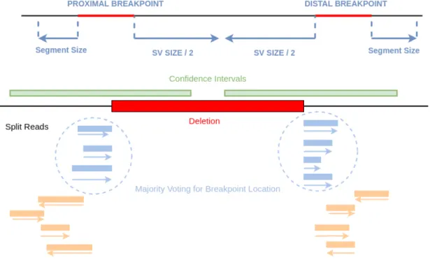
Figure 2.4: Clustering and majority voting of candidate breakpoint locations. We extract signaling split reads from extended SV confidence intervals. Each split read signals to a candidate breakpoint location that is calculated from its CIGAR string. Then, within each cluster, we vote candidate locations by the reads supporting to it. Finally, we predict candidate location with the highest support as the final breakpoint.

Chapter 3

Results

In this chapter, we evaluate the performance of BROSV using simulated data. We used 3 SV discovery tools, namely TARDIS, DELLY and LUMPY to discuss refinement performance of BROSV. We compared the number of false positives, false negatives and number of correctly refined predictions for these tools. While for DELLY and LUMPY our experiments are limited with deletions, inversions and tandem duplications, for TARDIS we also evaluate performance on inter-spersed duplications. Since there is no available tool for breakpoint refinement using HTS data, we compared our results with truth files of simulated data.

3.1

Simulated Data

We used VarSim [63] and CNVSim [50] to generate our simulation data. Even tough VarSim simulates deletions, inversions and tandem duplications by insert-ing known SVs to a reference sequence, it does not support simulation of inter-spersed duplications. Therefore, we used CNVSim, a recently developed sim-ulator for direct and invert interspersed duplications. CNVSim selects variant sizes uniformly between 500 bps and 10 Kbp and the distance between copies for interspersed duplications are selected uniformly between 5,000 bps and 50 Kbp

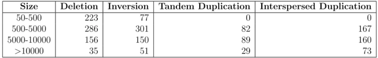
[50]. Second copy can be either on left or right at the predetermined random distance. CNVSim ensures that there is no assembly gap at the selected region and that the regions are non-overlapping. Table 3.1 illustrates the variant size distribution of simulated data for each SV type. For interspersed duplications, 200 of the simulated variants are inverted and remaining 200 are direct.

Table 3.1: Size distribution of variants in simulated data for each SV type.

Size Deletion Inversion Tandem Duplication Interspersed Duplication

50-500 223 77 0 0

500-5000 286 301 82 167

5000-10000 156 150 89 160

>10000 35 51 29 73

Table 3.2 shows the refinement performance of BROSV for deletions on simu-lated data. There are 527 imprecise deletions reported by TARDIS. Since we try to refine TARDIS SV predictions, it should be the point of reference. Each row shows percentange and the number of correctly predicted breakpoints for both proximal (left) and distal (right) breakpoints within allowed error margin. For example; first row shows number of breakpoints predicted with no error. Simi-larly, next row shows correct predictions within 1 base away from true location of SV breakpoint. Likewise, Table 3.3, Table 3.4 and Table 3.5 illustrates the refinement performance of BROSV for inversions, tandem duplications and in-terspersed duplications respectively. In Table 3.5 extra column (copy) stands for the prediction results for the location of the second copy.

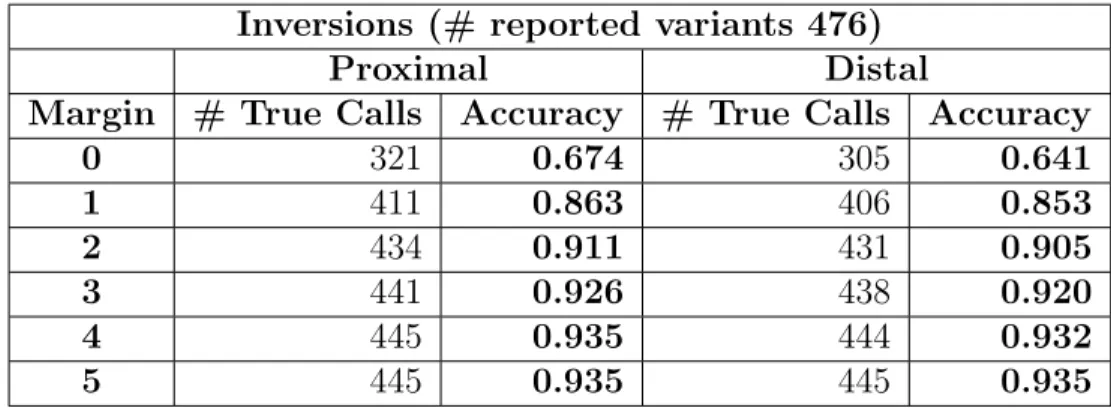
As seen in Table 3.2, BROSV refines 527 imprecise TARDIS deletion pre-dictions. Out of 457, breakpoints of 445 imprecise variants are correctly refined to 5 base pair resolution. Similarly, 445 of 476 inversions, 168 of 178 tandem repeats and 333 of 348 interspersed duplications that BROSV reported are cor-rectly refined with 5 base pair error margin (See Table 3.3, 3.4, 3.5). In other words, BROSV achieves 0.97, 0.93, 0.94, 0.95 refinement precision for deletions, inversions, tandem and interspersed duplications respectively.

Table 3.2: Refinement performance of BROSV for deletions using simulated data. Deletions (# reported variants 457)

Proximal Distal

Margin # True Calls Accuracy # True Calls Accuracy

0 322 0.705 348 0.761 1 410 0.897 415 0.908 2 430 0.941 435 0.951 3 438 0.958 445 0.973 4 442 0.967 446 0.975 5 445 0.973 446 0.975

Table 3.3: Refinement performance of BROSV for inversions using simulated data.

Inversions (# reported variants 476)

Proximal Distal

Margin # True Calls Accuracy # True Calls Accuracy

0 321 0.674 305 0.641 1 411 0.863 406 0.853 2 434 0.911 431 0.905 3 441 0.926 438 0.920 4 445 0.935 444 0.932 5 445 0.935 445 0.935

Table 3.2, 3.3, 3.4 and 3.5 also reveals that almost all of the refined breakpoints are within 1 base pair error margin. After that only a few new breakpoints contribute to the existence results. This is notable because even if we allow 5 base pair error margin for experimentation purposes, distribution of the results concentrates heavily on 0-1 error, fulfilling the promise of exact breakpoints.

Table 3.6 shows the overall performance of BROSV for TARDIS predictions. We report the number of SVs in simulated data, total number of calls made by TARDIS and BROSV, number of true positives, false negatives and false positives for each SV type. Note that upper limit for total number of calls made by BROSV is total number of calls made by TARDIS. For BROSV true positive

Table 3.4: Refinement performance of BROSV for tandem duplications using simulated data.

Tandem duplications (# reported variants 178)

Proximal Distal

Margin # True Calls Accuracy # True Calls Accuracy

0 120 0.674 127 0.713 1 157 0.882 157 0.882 2 167 0.938 166 0.932 3 168 0.944 168 0.944 4 168 0.944 168 0.944 5 168 0.944 169 0.949

Table 3.5: Refinement performance of BROSV for interspersed duplications using simulated data.

Interspersed Duplications (# reported variants 348)

Proximal Distal Copy

Margin # True Calls Accuracy # True Calls Accuracy # True Calls Accuracy

0 239 0.687 259 0.744 248 0.713 1 313 0.899 311 0.893 318 0.913 2 324 0.931 324 0.931 333 0.956 3 330 0.948 327 0.940 336 0.965 4 333 0.956 333 0.956 336 0.965 5 333 0.956 333 0.956 336 0.965

(TP) indicates the number of correctly refined variants. A variant is considered as refined if BROSV improved its breakpoint resolution up to 5 base pairs. We also reported false positives (FP) and false negatives (FN) for original TARDIS predictions and for BROSV refinement results. A false positive for BROSV means that even if it reports an SV breakpoint for specified SV type at a location, reported SV either does not exist, or its type is different, or its location is off more than 5 base pairs. Note that for BROSV false negative (FN) implies that the breakpoints of the predicted variant cannot be refined up to 5 base pair resolution with adequate support. The reported FN count is bounded by the SV discovery tool’s recall rate. In other words, BROSV ’s FN count is accumulated on TARDIS’s FN count because it is not possible to refine an SV if it is not

Table 3.6: Overall performance of BROSV for TARDIS predictions.

TARDIS BROSV

True calls # calls TP FN FP # calls TP FN FP

Deletion 700 574 572 128 2 457 454 256 3

Inversion 579 492 472 107 20 476 463 116 13

Tandem duplication 200 203 193 7 10 178 169 31 9

Interspersed duplication 400 399 388 12 11 348 339 61 9

reported by the SV caller.

BROSV refines 457 of 572 deletions, 463 of 472 inversions, 169 of 193 tandem repeats, and 339 of 388 interspersed duplications among imprecise TARDIS pre-dictions up to 5 base pair breakpoint resolution. It is a significant improvement when we consider the information in the Table 3.6, Figure 3.1 and 3.2 together. On one hand, we have confidence intervals between 300-500 base pairs, meanwhile BROSV offers exact breakpoints for significant number of those predictions. It is useful to remark that majority of reported exact breakpoints are off at most 1 base pair from their true genomic location (See Figure 3.1 and 3.2).

Table 3.7: Overall performance of BROSV for DELLY predictions.

DELLY BROSV

True calls # calls TP FN FP # calls TP FN FP

Deletion 700 922 627 73 295 742 502 198 240

Inversion 579 692 491 88 201 480 338 241 142

Tandem duplication 200 393 195 5 198 363 168 32 195

Table 3.8: Overall performance of BROSV for LUMPY predictions.

LUMPY BROSV

True calls # calls TP FN FP # calls TP FN FP

Deletion 700 773 587 113 186 652 477 223 175

Inversion 579 458 455 124 3 445 442 137 3

Tandem duplication 200 380 189 11 191 354 165 35 189

Table 3.7 and Table 3.8 shows the total number of predictions made by DELLY, LUMPY and BROSV, number of true positives, false negatives and false posi-tives for each SV type. Unlike TARDIS, these tools do not support interspersed duplication discovery. They also have high false discovery rate and high num-bers of false positives. As described earlier, TP for BROSV means number of correctly refined variants, FP indicates number of incorrrectly refined variants or FPs of DELLY/LUMPY that could not be eliminated. Finally, FN for BROSV represents that sufficient support for refinement could not be provided for that imprecise variant. It is bounded by recall of discovery tool whose predictions are employed.

BROSV correctly refines 502 of 627 deletions, 338 of 491 inversions and 168 of 195 tandem repeats among imprecise DELLY predictions. It also eliminates reasonable number of false positive calls, especially for inversions (See Table 3.7). For LUMPY predictions, while BROSV refines 477 of 587 deletions , 442 of 455 inversions and 165 of 189 tandem repeats, it does not offer a considerable improvement on number of false positives. Note that we take the SV caller’s (DELLY or LUMPY) TP count as the point of reference since best possible refinement performance would be refining all variants correctly reported by the SV caller.

Table 3.9: Precision, recall and F1 scores of BROSV on simulated data.

TARDIS DELLY LUMPY Precision Recall F1 score Precision Recall F1 score Precision Recall F1 score Deletion 0.993 0.780 0.873 0.676 0.801 0.733 0.732 0.827 0.776 Inversion 0.973 0.981 0.977 0.704 0.688 0.696 0.993 0.971 0.982 Tandem duplication 0.949 0.885 0.916 0.463 0.862 0.602 0.466 0.873 0.608 Interspersed duplication 0.974 0.874 0.921 - - -

-Table 3.9 presents the precision, recall and F1 scores of BROSV for TARDIS, DELLY and LUMPY predictions. Recall values are equal to T P

T P +F N where FN

is the difference between number of false negatives of the SV caller and BROSV since BROSV is only responsible for the variants reported by the SV caller. Precision values for TARDIS predictions are better than other tools’ since DELLY and LUMPY have much higher numbers of false positives than TARDIS and BROSV cannot eliminate their false positives. In this sense, its performance is highly dependent on the SV callers performance. Moreover, precision of tandem

Figure 3.1: Size distribution of confidence intervals of proximal breakpoints. Y axis shows the confidence interval size of each TARDIS prediction. X axis corre-sponds the final refinement result of BROSV for each prediction.

duplications for DELLY and LUMPY calls are around 46% as a result of their high false positive counts. BROSV needs to employ stricter criteria for signaling read selection to discard false positive calls for duplications. One solution may be adoption of read pair analysis to obtain more reliable evidence. Another solution can be sequence assembly by using both split reads and other discordant reads.

Figure 3.1 and 3.2 shows the size distribution of confidence intervals for TARDIS deletion predictions before and after BROSV refinement for proximal and distal breakpoints respectively. Y axis demonstrates the size of confidence intervals for initial TARDIS predictions and X axis show the size of error mar-gin after BROSV refinement for each correctly refined variant. While TARDIS generally offers confidence intervals between 200-400 base pairs, with BROSV refinement exact breakpoints are known with 5 base pair error margin.

Figure 3.2: Size distribution of confidence intervals of distal breakpoints. Y axis shows the confidence interval size of each TARDIS prediction. X axis corresponds the final refinement result of BROSV for each prediction.

Finally, in majority voting step, there are cases where few candidate locations get similar split read support. Table 3.10 presents some examples for tie scenarios in voting. In our current setting, BROSV only favors the location with the highest split read support. As a result, cases presented in Table 3.10 are discarded. The information provided by those split reads supporting the candidate location with the second highest votes is not utilized, that in fact indicates the true genomic location of the breakpoint in question.

Figure 3.3 and Figure 3.4 illustrates the number of correctly refined break-points (with 0 error margin) for deletions and inversions (TARDIS predictions) respectively when top ranked and second ranked candidate location is chosen. For deletions, 322 proximal and 348 distal breakpoints are refined when top ranked location is chosen. Additionally, only 3 proximal and 1 distal breakpoints are refined when second ranked location is chosen. However, for inversion, second ranked candidate locations offer more improvement. While 320 proximal break-points are refined by choosing top ranked locations, 68 more breakbreak-points are

Figure 3.3: Number of deletion breakpoints refined by using top ranked and second ranked candidate location in majority voting.

Figure 3.4: Number of inversion breakpoints refined by using top ranked and second ranked candidate location in majority voting.

Table 3.10: Example tie cases in majority voting. In voting step, some candidate locations get similar high split read support. Each row represents a candidate location for an SV breakpoint. While first row represents the top ranked location, second row represents the second ranked candidate location etc. True location for each example SV breakpoint is shown in bold. BROSV selects top ranked candidate location in our current setting. Although in these cases, actually second ranked locations reflect the true genomic loci of the breakpoint.

SV type Chromosome Position # votes

Deletion 1 37557419 8 37557420 5 5 12820338 7 12820330 6 12 7968671 10 7968677 7 Inversion 16 85190144 15 85190143 13 16 85187345 14 85187346 13

correctly located when we consider second ranked locations. Moreover, on top of 309 distal breakpoints refined with top ranked candidate locations, 96 additional distal breakpoints are refined by choosing second ranked locations. In total, 388 proximal and 405 distal breakpoints are correctly refined by utilizing the top and second ranked candidate locations in majority voting for inversions.

Chapter 4

Discussion and Future Work

In this thesis, we present BROSV a breakpoint refinement algorithm for genomic structural variation. While current SV discovery tools using HTS data are able to detect all kinds of SVs accurately, they usually disregard the task of finding the exact breakpoint location of the predicted variants. BROSV can pinpoint the true location of SV breakpoints using any discovery tools predictions with high precision for all sizes of variants. It also eliminates the reasonable numbers of false positive calls for TARDIS and DELLY. However, its validation performance is limited for LUMPY, namely, it is not able to eliminate false predictions. Another issue with BROSV is that since it uses only split read analysis and does not make use of read pair information, breakpoints of some predicted SVs cannot be refined with adequate support. As a result, it increases the number of false negatives. We address these issues in the following sections with possible future directions for BROSV.

4.1

Local Assembly for Refinement

In order to utilize read pair information in regions of SV events, we can extract discordant read pairs from confidence intervals for each SV as well as split reads.

By performing local assembly on reads in each interval, then realigning the result-ing contigs to the relevant part of the reference genome, we can refine breakpoints for imprecise SV calls. Also this approach can provide a better performance on false positive elimination since resulting contigs would cover a wider region of genome that will reduce mapping ambiguity. Even tough we tried local assembly in our experiments, we were unable to obtain a meaningful results due to low quality and short contigs. This approach can be revisited with a higher coverage data.

4.2

Multiple Sequence Alignment

Similar to the local assembly method, multiple sequence alignment can also be used to utilize read pair information. Multiple sequence alignment is the task of aligning two or more related sequences with each other. We can extract discordant read pairs and split reads from confidence intervals forming clusters. Then for each cluster, multiple sequence alignment can be applied to reveal the common signal on SV breakpoint location.

4.3

Local Assembly for Novel Insertions

While we experimented with deletions, inversions and duplications, we do not perform any test on novel insertions. While a similar methodology can be used for breakpoint refinement, local assembly is needed to attain the content of inserted novel sequence. For this purpose, all split reads that are mapped to breakpoint regions of insertions should be extracted. Then, all the orphan and OEA (one end anchored) reads can be clustered to match these groups of reads to an insertion event. Finally, reads in these clusters can be assembled to obtain the novel inserted sequence.

4.4

Improvement in Voting Step

As discussed in Results section of the thesis, we have cases where some can-didate locations have high and similar numbers of split read support. In our current setting, we choose the location with the highest split read vote as the final breakpoint prediction. In order to utilize the information provided by split reads supporting the candidate locations with the high number of votes, and not only the top candidate, a probabilistic approach can be appointed. Instead of favoring the location that has the highest support with majority voting, votes of each split read can be weighed with respect to the length and quality of its matched sequence. Thus, the reported results would be more reliable by mak-ing use of all the information available instead of discardmak-ing it. Also, a weighed voting approach would help to resolve tie cases.

4.5

Genotyping

Genotyping is the task of determining the differences of a sample genome with the reference genome. In our case, it is the task of determining whether a previously discovered variant exist in the sample genome or not. SV discovery and geno-typing is crucial to understand genomic disease associations. Ideally, this task requires accurate prediction of three aspects of SVs: copy, content and structure [1]. However, it remained elusive due to the challenges explained earlier such as repetitive nature of the genome (See Section 2.2). Since BROSV improve break-point resolution, we know the exact location of an SV (with 5 base pair error margin), it eases the genotyping process by reducing the target loci for possible genomic changes (SVs).

4.6

Application to Real Datasets

BROSV ’s performance can be tested on real data as well as simulation data. For these experiments, publicly available datasets such as the haploid human genome cell lines CHM1, CHM13 [64, 65] and diploid genome NA12878 can be utilized. For future directions, BROSV can be used to refine 1000 Genome Project [56] data and evaluate and improve its performance.

BROSV can be incorporated with alignment free structural variation geno-typers like Nebula [66] and Hawk [67] with the aid of refined exact breakpoints. By this way, extensive computational workload to genotype newly sequenced samples can be evaded. These large real datasets can also be integrated with graph aligners like [68], VG [69], HISAT2 [70] once they are resolved/refined with BROSV.

Bibliography

[1] C. Alkan, B. P. Coe, and E. E. Eichler, “Genome structural variation dis-covery and genotyping,” Nature Reviews Genetics, vol. 12, no. 5, p. 363, 2011.

[2] I. Hajirasouliha, F. Hormozdiari, C. Alkan, J. M. Kidd, I. Birol, E. E. Eichler, and S. C. Sahinalp, “Detection and characterization of novel sequence inser-tions using paired-end next-generation sequencing,” Bioinformatics, vol. 26, no. 10, pp. 1277–1283, 2010.

[3] International SNP Map Working Group, “A map of human genome sequence variation containing 1.42 million single nucleotide polymorphisms,” Nature, vol. 409, no. 6822, p. 928, 2001.

[4] K. K. Wong, R. J. deLeeuw, N. S. Dosanjh, L. R. Kimm, Z. Cheng, D. E. Horsman, C. MacAulay, R. T. Ng, C. J. Brown, E. E. Eichler, et al., “A comprehensive analysis of common copy-number variations in the human genome,” The American Journal of Human Genetics, vol. 80, no. 1, pp. 91– 104, 2007.

[5] P. Stankiewicz and J. R. Lupski, “Genome architecture, rearrangements and genomic disorders,” TRENDS in Genetics, vol. 18, no. 2, pp. 74–82, 2002.

[6] B. B. de Vries, R. Pfundt, M. Leisink, D. A. Koolen, L. E. Vissers, I. M. Janssen, S. van Reijmersdal, W. M. Nillesen, E. H. Huys, N. de Leeuw, et al., “Diagnostic genome profiling in mental retardation,” The American Journal of Human Genetics, vol. 77, no. 4, pp. 606–616, 2005.

[7] A. J. Sharp, S. Hansen, R. R. Selzer, Z. Cheng, R. Regan, J. A. Hurst, H. Stewart, S. M. Price, E. Blair, R. C. Hennekam, et al., “Discovery of previously unidentified genomic disorders from the duplication architecture of the human genome,” Nature Genetics, vol. 38, no. 9, p. 1038, 2006.

[8] J. Sebat, B. Lakshmi, D. Malhotra, J. Troge, C. Lese-Martin, T. Walsh, B. Yamrom, S. Yoon, A. Krasnitz, J. Kendall, et al., “Strong association of de novo copy number mutations with autism,” Science, vol. 316, no. 5823, pp. 445–449, 2007.

[9] D. Malhotra and J. Sebat, “CNVs: harbingers of a rare variant revolution in psychiatric genetics,” Cell, vol. 148, no. 6, pp. 1223–1241, 2012.

[10] F. Mitelman, B. Johansson, and F. Mertens, “The impact of translocations and gene fusions on cancer causation,” Nature Reviews Cancer, vol. 7, no. 4, p. 233, 2007.

[11] A. J. Iafrate, L. Feuk, M. N. Rivera, M. L. Listewnik, P. K. Donahoe, Y. Qi, S. W. Scherer, and C. Lee, “Detection of large-scale variation in the human genome,” Nature Genetics, vol. 36, no. 9, p. 949, 2004.

[12] E. Tuzun, A. J. Sharp, J. A. Bailey, R. Kaul, V. A. Morrison, L. M. Pertz, E. Haugen, H. Hayden, D. Albertson, D. Pinkel, et al., “Fine-scale structural variation of the human genome,” Nature Genetics, vol. 37, no. 7, p. 727, 2005.

[13] A. M. Maxam and W. Gilbert, “A new method for sequencing DNA,” Pro-ceedings of the National Academy of Sciences, vol. 74, no. 2, pp. 560–564, 1977.

[14] F. Sanger, S. Nicklen, and A. R. Coulson, “DNA sequencing with chain-terminating inhibitors,” Proceedings of the National Academy of Sciences, vol. 74, no. 12, pp. 5463–5467, 1977.

[15] J. A. Reuter, D. V. Spacek, and M. P. Snyder, “High-throughput sequencing technologies,” Molecular Cell, vol. 58, no. 4, pp. 586–597, 2015.

[16] F. Sanger and A. R. Coulson, “A rapid method for determining sequences in DNA by primed synthesis with DNA polymerase,” Journal of Molecular Biology, vol. 94, no. 3, pp. 441–448, 1975.

[17] International Human Genome Sequencing Consortium, “Initial sequencing and analysis of the human genome,” Nature, vol. 409, no. 6822, p. 860, 2001. [18] International Human Genome Mapping Consortium, “A physical map of the

human genome,” Nature, vol. 409, no. 6822, p. 934, 2001.

[19] J. M. Churko, G. L. Mantalas, M. P. Snyder, and J. C. Wu, “Overview of high throughput sequencing technologies to elucidate molecular pathways in cardiovascular diseases,” Circulation Research, vol. 112, no. 12, pp. 1613– 1623, 2013.

[20] H. Li, B. Handsaker, A. Wysoker, T. Fennell, J. Ruan, N. Homer, G. Marth, G. Abecasis, and R. Durbin, “The sequence alignment/map format and sam-tools,” Bioinformatics, vol. 25, no. 16, pp. 2078–2079, 2009.

[21] C. Firtina and C. Alkan, “On genomic repeats and reproducibility,” Bioin-formatics, vol. 32, no. 15, pp. 2243–2247, 2016.

[22] T. J. Treangen and S. L. Salzberg, “Repetitive DNA and next-generation sequencing: computational challenges and solutions,” Nature Reviews Ge-netics, vol. 13, no. 1, p. 36, 2012.

[23] B. Langmead, C. Trapnell, M. Pop, and S. L. Salzberg, “Ultrafast and memory-efficient alignment of short DNA sequences to the human genome,” Genome Biology, vol. 10, no. 3, p. R25, 2009.

[24] C. Alkan, J. M. Kidd, T. Marques-Bonet, G. Aksay, F. Antonacci, F. Hor-mozdiari, J. O. Kitzman, C. Baker, M. Malig, O. Mutlu, et al., “Person-alized copy number and segmental duplication maps using next-generation sequencing,” Nature Genetics, vol. 41, no. 10, p. 1061, 2009.

[25] F. Hach, F. Hormozdiari, C. Alkan, F. Hormozdiari, I. Birol, E. E. Eichler, and S. C. Sahinalp, “mrsFAST: a cache-oblivious algorithm for short-read mapping,” Nature Methods, vol. 7, no. 8, p. 576, 2010.

[26] H. Xin, D. Lee, F. Hormozdiari, S. Yedkar, O. Mutlu, and C. Alkan, “Accel-erating read mapping with FastHASH,” in BMC Genomics, vol. 14, p. S13, 2013.

[27] NovoAlign. Available at: http://www.novocraft.com/. Accessed 08-2019.

[28] B. Langmead and S. L. Salzberg, “Fast gapped-read alignment with Bowtie 2,” Nature Methods, vol. 9, no. 4, p. 357, 2012.

[29] H. Li and R. Durbin, “Fast and accurate short read alignment with Burrows– Wheeler transform,” Bioinformatics, vol. 25, no. 14, pp. 1754–1760, 2009.

[30] X. Fan, T. E. Abbott, D. Larson, and K. Chen, “BreakDancer: Identifica-tion of genomic structural variaIdentifica-tion from paired-end read mapping,” Current Protocols in Bioinformatics, vol. 45, no. 1, pp. 15–6, 2014.

[31] R. E. Handsaker, J. M. Korn, J. Nemesh, and S. A. McCarroll, “Discov-ery and genotyping of genome structural polymorphism by sequencing on a population scale,” Nature Genetics, vol. 43, no. 3, p. 269, 2011.

[32] F. Hormozdiari, I. Hajirasouliha, P. Dao, F. Hach, D. Yorukoglu, C. Alkan, E. E. Eichler, and S. C. Sahinalp, “Next-generation VariationHunter: com-binatorial algorithms for transposon insertion discovery,” Bioinformatics, vol. 26, no. 12, pp. i350–i357, 2010.

[33] A. R. Quinlan, R. A. Clark, S. Sokolova, M. L. Leibowitz, Y. Zhang, M. E. Hurles, J. C. Mell, and I. M. Hall, “Genome-wide mapping and assembly of structural variant breakpoints in the mouse genome,” Genome Research, vol. 20, no. 5, pp. 623–635, 2010.

[34] A. Abyzov, A. E. Urban, M. Snyder, and M. Gerstein, “CNVnator: an approach to discover, genotype, and characterize typical and atypical CNVs from family and population genome sequencing,” Genome Research, vol. 21, no. 6, pp. 974–984, 2011.

[35] F. Kahveci and C. Alkan, “Whole-genome shotgun sequence CNV detection using read depth,” in Copy Number Variants, pp. 61–72, Springer, 2018.