Cash inventory management at automated teller machines under incomplete information

CASH INVENTORY MANAGEMENT

AT AUTOMATED TELLER MACHINES

UNDER INCOMPLETE INFORMATION

A THESIS

SUBMITTED TO THE DEPARTMENT OF INDUSTRIAL ENGINEERING

AND THE INSTITUTE OF ENGINEERING AND SCIENCES OF BILKENT UNIVERSITY

IN PARTIAL FULFILLMENT OF THE REQUIREMENTS FOR THE DEGREE OF

MASTER OF SCIENCE

by Yaşar Altunoğlu

I certify that I have read this thesis and that in my opinion it is fully adequate, in scope and in quality, as a thesis for the degree of Master of Science.

Asst. Prof. Dr. Alper Şen (Advisor)

I certify that I have read this thesis and that in my opinion it is fully adequate, in scope and in quality, as a thesis for the degree of Master of Science.

Asst. Prof. Dr. Osman Alp (Co-advisor)

I certify that I have read this thesis and that in my opinion it is fully adequate, in scope and in quality, as a thesis for the degree of Master of Science.

Prof. Dr. Nesim Erkip

I certify that I have read this thesis and that in my opinion it is fully adequate, in scope and in quality, as a thesis for the degree of Master of Science.

Asst. Prof. Dr. Pelin Bayındır

Approved for the Institute of Engineering and Sciences:

Prof. Dr. Mehmet Baray

ABSTRACT

CASH INVENTORY MANAGEMENT AT AUTOMATED TELLER MACHINES UNDER INCOMPLETE INFORMATION

Yaşar Altunoğlu M.S. in Industrial Engineering

Supervisors: Asst. Prof. Dr. Alper Şen, Asst. Prof. Dr. Osman Alp January 2010

Automated Teller Machines are one of the most important cash distribution channels for the banks. Since branches have more information about the ATM cash demand compared to headquarters, cash inventory at ATMs is usually managed by the branches. Inventory holding and stock-out costs, however, are incurred by the headquarters. We examine the headquarters’ cash inventory management problem for out of working hours under a Newsboy type setting. In this setting, inventory replenishment is not possible during the period and the headquarters cannot fully observe the amount of stock-outs. The headquarters seeks an inventory policy that would lead the branch to make ordering decisions to minimize the headquarters’ cost. We examine three policies: (M) policy with a lump-sum stock-out cost charged at the end of period, (t, M) policy with a lump-sum stock-out cost charged at time t within the period and (t, L, p) policy with a unit stock-out cost charged at time t within the period for inventory below L. Numerical analysis show that checking the inventory during the period - (t, M) and (t, L, p) policies - can lead to important reductions in cost for the headquarters.

Keywords: Automated Teller Machine, Cash Inventory Management,

ÖZET

OTOMATİK ÖDEME MAKİNELERİNDE EKSİK BİLGİ İLE NAKİT ENVANTER YÖNETİMİ

Yaşar Altunoğlu

Endüstri Mühendisliği Yüksek Lisans

Tez Yöneticileri: Yrd. Doç. Dr. Alper Şen, Yrd. Doç. Dr. Osman Alp Ocak 2010

Otomatik Ödeme Makineleri bankalar için en önemli nakit dağıtım kanallarından biridir. Banka şubeleri, banka merkezlerine göre nakit talebi hakkında daha fazla bilgiye sahip olduklarından, ATM’lerdeki nakit envanteri genelde şubeler tarafından yönetilmektedir. Ancak, envanter tutma ve yok-satma maliyetleri merkez aitttir. Bu çalışmada, merkezin mesai saatleri dışındaki nakit envanter problemi Gazeteci çocuk tipi bir çerçevede ele alınmış olup periyot boyunca stok yenileme ve yok-satma miktarını görme imkanı bulunmamaktadır. Merkez, şubeye kendi maliyetini en düşük yapacak sipariş kararlarını verdirecek bir envanter politikası aramaktadır. Bu çalışmada üç politika önerilmektedir: periyot sonunda sabit bir yok-satma cezasını öngören (M) politikası, periyot içerisinde t zamanında sabit bir yok-satma cezasını öngören (t, M) politikası ve t zamanında L’nin altında kalan stok miktarı için birim yok-satma cezasını öngören (t, L, p) politikası. Yapılan sayısal analiz, envanter düzeyinin periyot içerisinde kontrol edilmesinin - (t, M) ve (t, L, p) politikaları - merkezin maliyetlerinde önemli düşüş sağlayabileceğini göstermektedir.

Anahtar Kelimeler: Otomatik Ödeme Makinesi, Nakit Envanter Yönetimi,

ACKOWLEDGEMENT

I would like to express my sincere gratitude to my advisors Asst. Prof. Dr. Alper Şen and Asst. Prof. Dr. Osman Alp for their supervision, guidance, suggestions, encouragement, patience and insight throughout the research.

I am indebted to Prof. Dr. Nesim Erkip and Asst. Prof. Dr. Pelin Bayındır for devoting their valuable time to read and review this thesis and their substantial suggestions.

I would like to extend my special appreciation and gratitude to my family.

I would like to thank to my dear wife Sinem and my beautiful daughter Serra for being in my life.

TABLE OF CONTENTS

ABSTRACT... iii

ÖZET ... iv

ACKOWLEDGEMENT... vi

TABLE OF CONTENTS... vii

LIST OF TABLES... viii

1. INTRODUCTION... 1

2. LITERATURE REVIEW ... 8

3. MODEL FORMULATION... 14

3.1 Inventory Model with Full Information... 17

3.2 Inventory Model with Partial Information... 20

3.3 (t, M) Inventory Policy... 22 3.4 (t, L, p) Inventory Policy... 25 4. NUMERICAL ANALYSIS ... 28 4.1 (M) Inventory Policy ... 32 4.2 (t, M) Inventory Policy... 34 4.3 (t, L, p) Inventory Policy... 36

5. CONCLUSION AND FUTURE RESEARCH DIRECTIONS... 40

LIST OF TABLES

Table 1: Use of ATMs in Turkey ……… Table 2: Problem Settings for Numerical Analysis ………..……… Table 3: Exact Optimum Solutions for Headquarters ……….………. Table 4: Optimum Solutions for (M) Inventory Policy .………. Table 5: Optimum Solutions for (t, M) Inventory Policy …………..……….. Table 6: Optimum Solutions for (t, L, p) Inventory Policy ………..……….. Table 7: % Deviations from Optimum Solutions ..……….……….

4 31 32 34 35 37 38

Chapter 1

INTRODUCTION

The use of Automated Teller Machines (ATM) has increased over the years and ATMs have become one of the important banking service channels. Banks are expanding their ATM network to meet market demand and are facing operating costs and benefits together. ATMs are similar to small bank branches, which provide limited service without full time bank employees. From this perspective, ATMs are alternative media for simple banking transactions. Compared to crowded bank branches with long queues, people prefer to use ATMs for their simple daily transactions especially for cash withdrawals. Although some more complicated banking transactions and even credit applications can be handled by ATMs, people see ATMs mostly as cash dispensers. The increasing use of Internet banking shadowed interactive functions of ATMs. A new technology, BiAutomated Teller Machines (BTM), permit instant cash depositing in addition to cash withdrawal. But due to high installation costs and complicated operating requirements, the use of BTMs is not as pervasive as ATMs.

As a cash withdrawal media, ATMs have two basic functions. During working hours, ATMs are alternative cash withdrawal channels against the branches. During working hours, customers use ATMs for their cash need at the places where there is not a branch of a bank. Customers also use ATMs

the branch. This use of ATMs is an important avenue for cost reduction for the banks. With ATMs, branch employees of the banks can devote their time to more profitable services such as credit transactions instead of cash operations. Additionally, banks do not need to open a branch at every corner where the cash is needed; they just install an ATM at that corner. The branches are responsible for operating the ATMs in front of their building and ATMs at the corners in coverage of their branches. Within working hours, it is easy and less costly to operate the ATMs. A branch can continuously monitor its ATMs and manage their cash inventory. As stocks decrease, they can have ATMs loaded by branch employees with the money circulating in the branch. Branch will not face important safety risks owing to safety personnel of the branch who will assist the cash loading operation. A fully loaded ATM will not be prone to robbery attempts within working hours either. Moreover, cash does not bear any interest cost within working hours. These factors decrease the holding cost of cash within working hours. In case of an unloaded ATM, most of the customers will proceed to the nearest branch to withdraw money from their deposits or credit accounts. So stock-out cost is less likely and not very crucial within working hours. As a result, ATMs can be operated within working hours efficiently and with negligible costs and the personnel may be profitably diverted to other operations.

A more difficult to manage function of ATMs is cash withdrawals out of working hours. (Working hours of bank branches are usually similar to official working days from morning to evening.) Most of the bank branches are closed at nights and weekends. So at these times, ATMs become the sole cash withdrawal media for the public. This creates a different cash inventory management framework for ATMs. Firstly, within working hours, banks can

demand cash from central bank without paying interest as long as they return the cash before working hours end. But, cash deposited to the central bank at the evening earns an overnight interest including the weekends. For the cash loaded to the ATMs for the night and weekend, the banks forego this interest earning. Secondly, especially for the nights, cash loaded to ATMs is more prone to robbery attempts leading to high insurance costs. For the money withdrawn by the costumers, banks usually make transaction profits more than the interest and insurance cost mentioned above. Profit arises from the banking services such as time deposits, credit cards, exchange services and investment accounts. Profit margins of some of these transactions out of working hours are significantly higher than those during working hours.

The stock-out of ATMs at nights or weekends is more crucial compared to working hours for the banks. First of all, reloading of ATMs at nights or weekends is not possible for the branches, as they do not work at these times. Banks can have special units to load their ATMs out of working hours or outsource these loading services to companies specialized in cash services to banks. Such services within the bank or from an outside company are very costly due to safety risks. These services may help to reduce the insurance cost; however, the interest costs are still there, as the money has to be spared for the night. Since these services are expensive, the savings associated with such services are rather insignificant. Moreover, safety risks are more important than costs for the banks, as they do not want to be defamed with occasions such as robbery attempts. Hence, except a few ATMs in safer locations such as shopping centers, banks will not prefer to reload ATMs during nights and weekends. If banks face a capacity problem for an ATM at a specific location, they do not hesitate to install more than one ATM at the same location, instead of reloading out of working hours.

In the absence of reloading, stock-out of ATMs out of working hours is a serious problem for the banks. Banks can associate this problem with stock-out costs, which can be quantified rather easily. Firstly, banks lose possible profitable transactions like cash withdrawn by credit cards. Banks earn more than ten times of the interest cost for the cash withdrawn by credit cards. Secondly, customer satisfaction is very sensitive to such stock-out cases. Nights and weekends are the periods when people need more cash as the consumption is more at these times. If someone has a deposit account at a bank or a credit card of a bank, he will want to be sure that he will be able to use his money at any time. If a customer faces frequent stock-outs at the ATMs of a specific bank, he will not hesitate to change his bank in such a competitive sector.

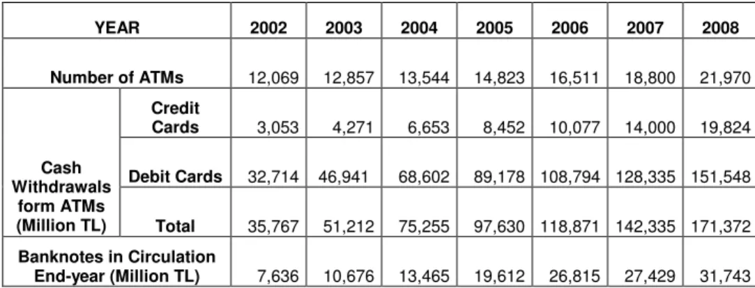
To understand the macroeconomic significance of ATMs, the trend in the use of ATMs in Turkey will be helpful (See Table 1). It can be seen that within 6 years, the number of ATMs in Turkey almost doubled. The total amount of cash withdrawn from ATMs has been about five times banknotes in circulation each year.

YEAR 2002 2003 2004 2005 2006 2007 2008 Number of ATMs 12,069 12,857 13,544 14,823 16,511 18,800 21,970 Credit Cards 3,053 4,271 6,653 8,452 10,077 14,000 19,824 Debit Cards 32,714 46,941 68,602 89,178 108,794 128,335 151,548 Cash Withdrawals form ATMs (Million TL) Total 35,767 51,212 75,255 97,630 118,871 142,335 171,372 Banknotes in Circulation End-year (Million TL) 7,636 10,676 13,465 19,612 26,815 27,429 31,743

(The Interbank Card Center, http://www.bkm.com.tr/bkm-en/periodic-data.aspx) Table 1: Use of ATMs in Turkey

Banks operate via their self-owned branches and all the costs and profits associated from branch operations belong to the headquarters of the bank. Branches are evaluated based on their profit performance and branch managers and employees are paid, prized and nominated according to this performance. For the case of ATMs, however, the cost and profit accountability is different than other branch operations. Most of the customers served by the ATMs do not have deposit accounts at the branch that is operating the ATM. Thus, the costs and profits incurred for ATM operations directly belong to the headquarters. For example, branches have nothing to do with ATM credit card revenues of headquarters. Branches are also not directly affected by general ATM customer satisfaction levels of the bank. But branches have an information advantage: they tend to know more about the cash demand of their local coverage. Due to the physical proximity and constraints, banks prefer branches to operate ATMs on behalf of the headquarters. Operating the ATMs includes loading and unloading cash from the ATMs. At that level, the amount of cash that will be loaded at the start of the period (night or weekend) is the most crucial decision. Either the headquarters will determine or will let the branches decide the amount of cash to be loaded. Headquarters has the past statistics about the ATM cash withdrawals to infer the general demand distribution. But, local effects and other information can only be obtained by branches. Gathering such qualitative information from the branches is not a very easy process. Such information cannot be easily integrated to decision support systems. Thus, most of the banks prefer their branches to determine the amount of cash that will be loaded to ATMs. So headquarters should adopt a proper incentive and evaluation system to ensure that branches manage ATM cash inventory efficiently.

There are also banks that rely on past statistics ignoring local information and manage the cash inventory centrally. Headquarters dictate the amount of cash that will be loaded to each ATM by the branches. Managing cash inventory at this detail may not be appropriate for headquarters of the banks. Headquarters are expected to manage and monitor the other units of banks; to direct them to perform operational functions efficiently. Therefore such central inventory management systems may lead to inefficiencies and costs, in addition to loss of local information.

High underage and overage costs make ATM cash inventory management crucial for banks. Due to decreasing profit margins, increasing competition, banks will not want to lose profit and market share due to mismanagement of cash inventory. Our objective in this thesis is to evaluate the decision making processes to minimize operating costs and provide optimum or near optimum cash inventory management solutions for the banks.

It should also be noted that the inventory problem discussed here can also be valid for sectors other than banking. In industries in which local distributors or representatives operate on behalf of their suppliers, inventory management can be done locally especially in the case of asymmetric information. The problem faced by the suppliers is similar to what the bank headquarters face: design of mechanisms and incentives for the local distributors or representatives such that they manage the local inventory efficiently on their behalf.

In this thesis, we propose two new inventory policies that can be adopted by the headquarters such that the branches can manage the ATM inventory more efficiently on behalf of the headquarters. The first policy reviews the

inventory at a time t before the period ends and charges a lump-sum cost of

M for a stock-out occasion (in addition to the inventory holding cost at the

end of the period). The second policy also reviews the inventory at a time t before the period ends, but charges a unit stock-out cost if the inventory is below a threshold level. Both policies provide the advantage of observing the system before the end of period over a traditional baseline policy in which the inventory is reviewed only at the end of the period and a lump-sum cost is charged for stock-out occasions (since the lost sales cannot be observed). In addition, the second policy provides the opportunity to individually account for possible stock-outs. We first derive the optimal branch response under these three policies (two new and one baseline). We also formulate the headquarters’ problem of the determining policy parameters such that its expected costs are minimized. We then compare the three policies under a variety of settings. Our results show that the two policies may provide significant cost reductions over the baseline policy.

The rest of the thesis is organized as follows. In Chapter 2, we review the related inventory literature. In Chapter 3, we propose our inventory policies and analyze the corresponding problems faced by the branch and the headquarters under these policies. In Chapter 4, we provide the results of a numerical study that compares the three inventory policies. Chapter 5 concludes the thesis with managerial insights for the ATM cash inventory management and possible avenues for future research.

Chapter 2

LITERATURE REVIEW

One of the first cash inventory problem problems was posed by Girgis (1968). In this paper, the author considers the optimal policies for keeping cash in anticipation of future net expenses. Starting with a beginning inventory level, decision maker is allowed to change the inventory level in any direction at the beginning of each period. In addition to the usual holding and shortage costs, the problem involves fixed and proportional costs for changing the inventory level. The paper derives the form of the optimal policy if the expected holding and shortage cost is convex and no fixed costs are involved for increasing or reducing the inventory.

The next study on the cash inventory problem is by Neave (1970). He studies a very similar cash inventory problem in which the stochastic cash inventory change could either be positive or non positive and decisions to increase or decrease the inventory is permitted at the beginning of each time period. Through an example the author demonstrates that when the costs are positive and the loss function is convex, a simple (s, S) policy is not optimal. The author also shows that a simple policy is optimal, when proportional costs of changing the inventory are zero, the two fixed cost are equal, the loss function is symmetric quasi-convex and the demand probability densities are quasi-concave. For the cases in which simple

polices are not optimal, the author develops a technique which employs convex upper and lower bounds on the non-convex cost functions partially to describe the optimal policy.

Noori and Bell (1982) study the cash inventory problem especially for the banking industry. They investigate the problem of foreign currency management at Canadian branch banks and identify an inventory problem that is closely related to the standard inventory problem but differs in two important aspects. First, demand is explicitly permitted to be negative and second, the shortage cost is assumed to be independent of the magnitude of shortage. After investigating data from 280 days of foreign currency operations at branch bank, they find that normal distribution is an appropriate approximation for the distribution of net demand. They derive the form of optimal polices and investigated the conditions under which such policies include an order. They obtain closed-form solutions for the case of uniformly distributed demand; but in the case the demand is normally distributed, they need numerical methods to compute optimal solutions.

Foreign currency inventory management problem is extended in another paper by Bell and Noori (1984). They extend their previous currency inventory model by adding an emergency order option to make up any potential within-period shortages. The expected total cost minimization problem over a finite horizon is formulated as a dynamic programming problem, which enables to find the minimum expected cost policy form the set of simple policies. They argue that such polices are often globally optimal under conditions found in branch banking. Further, their policies

are easy to understand the management and are potentially implementable. According to authors, cost savings from implementing such polices at a single branch is quite small. The fact that several Canadian banks have more than a thousand branches suggests that the potential benefits from system-wide implementation might be significant.

Studies discussed so far assumes that the unsatisfied demand can be backordered, the net demand can be negative and initial inventory options which are valid assumptions for cash inventory management for banks. But, for the ATM cash management, backordering and negative demand are not valid assumptions. For ATM cash inventory management, unsatisfied demand is lost and the exact amount of shortage cannot be observed. Therefore, ATM cash management problem differs from the problems studied in the traditional cash management literature and only recently received attention from researchers.

Smitus et al. (2007) presents an approach to cash management for ATM network. The approach is based on an artificial neural network to forecast a daily cash demand for every ATM in the network and on the optimization procedure to estimate the optimal cash load for every ATM. During the optimization procedure, the most important factors for ATMs maintenance are considered: cost of cash, cost of cash uploading and cost of daily services. Simulation studies show that in case of higher cost of cash (interest rate) and lower cost for money uploading, (the optimization procedure allowed decreasing the ATMs maintenance costs around 15-20 %). They suggest that for practical implementation of the proposed

ATMs’ cash management procedure, further experimental investigations are necessary.

Wagner (2007) develops a conceptual framework to derive the optimal cash deployment strategy for a network of ATMs and assessed potential benefits of sophisticated cash management software. The study applies an exploratory case study design, which is based on normative empirical research using discrete event simulation. A single case setting is used since the emphasis of the research question is on identifying the variables that impact the optimal cash deployment strategy, their effect size and interrelations rather than looking at the differences within the industry. A total of six experiments were designed to analyze the different degrees of optimization benefits and costs. The study shows that major cost savings up to 28 percent can be achieved by applying the Wagner-Whitin algorithm for optimal inventory allocation and Dantzig, Fulkerson & Johnson integer program for identifying routs of least total distance.

Cash inventory problems are specific versions of general inventory problems with lump-sum stock-out costs. Arrow et al. (1951) formulate the general inventory problem with a lump-sum stock-out penalty in addition to a unit stock-out cost. They derive best maximum stock and best reordering point as functions of the demand distribution, ordering costs and stock-out costs. Dyoretzky et al. (1952) also study the general inventory problem with a lump-sum stock-out penalty in addition to a unit stock-out cost. They showed that the optimum solution with lump-sum stock-out cost depends on the functional properties of the demand distribution. Bellman et al. (1955) discuss a number of functional

equations that arise in the optimal inventory problem. They derived existence and uniqueness theorems for the solutions of different inventory problems.

A study on fixed backorder costs came from Çetinkaya and Parlar (1998). They consider a single product, periodic review, stochastic demand inventory problem where backorders are allowed and penalized via fixed and proportional backorder cost simultaneously. They show that if the initial inventory was below S, a base stock level S policy is optimal regardless of model parameters and demand distribution. Otherwise, the sufficient condition for a myopic optimum requires some restrictions on demand density or parameter values. However, this sufficient condition is not very restrictive, in the sense that it holds immediately for Erlang demand density family. They also show that the value of S can be computed easily for the case of Erlang demand; they argue that this was important since most real-life demand densities with coefficient of variation not exceeding unity can well be represented with Erlang density. Thus, myopic policy might be considered as an approximation, if the exact policy was intractable.

Demand information is also an important topic discussed in inventory problem literature. Ananth and Bergen (1997) discuss Quick Response (QR), which is a movement in the apparel industry to shorten lead time. Under QR, the retailer has the ability to adjust orders based on better demand information. They studied how a manufacturer-retailer channel impacted choices of production and marketing variables under QR in the apparel industry. They build formal models of the inventory decisions of

manufacturer and retailers both before and after QR. Their model allows to address who won and who lost under QR, and to suggest actions such as service level, wholesale price and volume commitments that can be used to make QR profitable for both members of the channel.

Chapter 3

MODEL FORMULATION

The cash inventory management for ATMs can be modeled as a typical inventory control problem. However, one of the main characteristics of the ATM cash inventory problems is that the unsatisfied demand is lost and this lost demand cannot be observed. This is mostly due to the fact that ATMs inform the customers when it is out of stock. Banks do that not to annoy customers who will learn that ATM is out of cash after wasting some time with the machine at midnight. Banks also want to prevent ATMs from damage due to possible robbery attempts especially at nights. But branches always have good information about ATM cash demand on their coverage location. The stochastic demand for overnight or weekend cash demand can easily be approximated by some distributions by branches. Overnight or weekend cash demand distribution can also change day by day according to location specific properties. Branches also have the information to forecast such daily shifts in demand distribution parameters. Unfortunately, headquarters will not be able to follow daily shifts nor know the demand distribution of any specific day unless branches share exact information with them. The fact that most of the banks have over a thousand of branches also makes it difficult to obtain this information unless there is structured and well thought process.

Therefore, in this thesis, we assume that there is an information asymmetry between the headquarters and the branch with regards to cash demand at the ATM. We assume that the headquarters have only partial information about the demand observed by the ATMs at each branch. We assume that the headquarters know the general form of the demand distribution at the ATMs (for example, knows that it is Normally distributed) but they do not know exact parameters of the demand distribution; instead headquarters knows the distribution of parameters. Without exact specification of the demand distribution, the inventory problem faced by the headquarters is a complicated one as the headquarters cannot adopt an easy inventory control policy that would enforce the branch to operate in the favor of the its objectives.

We assume that the branch knows the exact information that which distribution will generate the demand at the time of loading. Note that this can easily be obtained by the branches if they load excess amount of cash in ATMs and observe the full demand for sufficiently number of times. The amount of the cash loaded to an ATM will be determined by the branch operating the ATM.

Under this asymmetric information and unobservable lost sales setting, we propose three policies that the headquarters can use such that the branch can manage the cash inventory on its behalf. These policies can be enforced as performance evaluation systems for the ATM cash inventory management of the branch. The headquarters can easily charge penalties for under- and over-stocking of cash. For the overage case, headquarters can charge the branch a unit holding cost. But for the underage case, as

lost demand can not be observed, headquarters can only charge the branch a lump-sum penalty cost in case of a stock-out, rather than charging a penalty proportional to the underage quantity.

The first policy is the simple policy denoted by (M) where M is the lump-sum cost charged by the headquarters to the branch in case the ATM is out-of-cash at the end of the period (night or weekend). The headquarters also charge a cost of h per unit of cash left over at the end of the period. The branch should try to find a load amount to minimize its total costs charged by the headquarters, whereas the headquarters determine the lump-sum penalty cost M so that the branch determines a load amount, which is also equal (or as close as possible) to the optimal load amount of the headquarters.

The (M) policy presents a baseline for how the headquarters manage their branches in practice. While this simple policy works properly for the case of full information and help the headquarters obtain the full information costs, it may lead to higher costs for the case of asymmetric information. Therefore, we propose two new policies. In (t, M) policy, the lump-sum penalty M is charged if the ATM is out of cash at time t before the end of period. In (t, L, p) a unit underage cost p is charged if the inventory at time t is below L. If there is a stock out at time t, a lump-sum cost of p*L is charged.

3.1 Inventory Model Under Full Information

In case of full information, as the headquarters knows all the demand distribution parameters with certainty, the inventory problem can easily be modeled as a typical single period inventory problem. There are underage and overage costs according to the inventory level at the end of night or weekend, say period. The lost demand can not be observed but its distribution is known and is enough for calculating expected shortage costs for a period. At the beginning of each period, an order quantity will be loaded to the ATM. This problem is also the problem that the headquarters would solve if they had the full control of the cash loading operations in ATMs. For each day of different demand characteristics, the headquarters will know the exact demand distribution and will solve this problem for each different day. Both headquarters and branch are assumed to be risk neutral; thus they will try to minimize their expected costs. Risk neutrality on such operational issues is a valid assumption for bankers. The following model, all subsequent models and the numerical analysis are based on this assumption.

h0 : inventory holding cost per unit left at the end of period

p0 : penalty cost per unit stock-out at the end of period

S : amount of cash loaded at the beginning of period

D : random variable denoting the demand during the period f : density function of demand during the period

F : distribution function of demand during the period

CH(S) : expected operating cost of headquarters for a period when amount of S is loaded

Headquarters’ problem is to find S to minimize

∫

∫

First order condition will be then

) /(

)

(S p₀ p₀ h₀

F _{= +} . (2) The second derivative is

) ( ) ( ) (S h₀f S p₀f S CH _{= +} , (3)

which is always positive for all S for a given h0, p0 and D.

If the headquarters knows the exact demand distribution, headquarters

would find the S* _{that satisfies (2) and minimizes (1). In theory, the}

headquarters may simply dictate the branch to load S* to the ATM. As mentioned before, in practice, the amount of the cash loaded to an ATM will be determined by the branch operating the ATM. The headquarters

can enforce an inventory policy that will lead the branch to the optimal S*

as loading amount. The inventory model here may be considered as a leader-follower game; headquarter sets internal parameters and the branch sets the inventory level to minimize its costs based on these parameters For this purpose, the headquarters can enforce a simple (M) policy where a lump-sum cost of M is charged to the branch if the ATM is out of cash at the end of the period. Under this policy, the branch would try to find a

load amount S to minimize total costs charged by the headquarters,

namely the lump-sum penalty cost and the holding costs charges for keeping excess amount of cash at the end of the period. We further define the following notation:

h : inventory holding cost per unit left at the end of period,

M : lump-sum penalty cost for stock-out at the end of period,

S : amount of cash loaded at the beginning of period,

CB(S) : expected operating cost of branch for a period when amount of S

is loaded.

Branch’s problem is to find S to minimize

∫

∫

First derivative using Leibniz’s rule

) ( ) ( ) ( 0 S Mf dx x f h S B C S

∫

hF(S)=Mf(S), (7) f(S)/F(S)=h/M . (8) The second derivative is

) ( ) ( ) (S hf S Mf S B C ′′ = − ′ . (9)

If we assume for the demand distribution that it satisfies the required first and second order conditions for all S for a given h, M and D, the branch

will find its optimum load amount S b_{that satisfies (8) and minimizes (4).}

So, the headquarters can determine h and M such that (8) will be satisfied

Headquarters can determine the h* _{and M}* _{such that:} * S Sb = , (10) * * * *_{)/ ( ) /} (S F S h M f ₌ . (11)

3.2 Inventory Model under Imperfect Information

The above inventory problem was based on the assumption that headquarters has the same level of information about the demand distribution as the branch has. Usually, this assumption does not hold and headquarters only knows the general distribution of the demand, but does not know distribution parameters exactly. To model this framework, it is

the assumed that there are n demand distributions D1

, D2,...., Dn which are identically and independently distributed random variables of same distribution type with different parameters. We also assume that the cash

demand is generated with distribution k with a probability pk _{at each}

period; where such probabilities sum up to 1. Unlike the headquarters, the branch exactly knows which distribution will generate the demand at the time of loading. The headquarters’ problem becomes more complicated.

h : inventory holding cost per unit left at the end of period

M : lump-sum penalty cost for stock-out at the end of t

Sk : amount of cash loaded at the beginning of period for demand

scenario Dk

Dk : demand during period for kth scenario k∈(1,...,n)

f k : kth possible density function of demand during the full period

) ,..., 1

( n

F k : kth possible distribution function of demand during the full period k∈(1,...,n)

Dtk : random variable denoting the demand generated from the kth

possible distribution during the period [0, t] k∈(1,...,n)

ftk : density function of Dtk during the period [0, t] k∈(1,...,n)

Ft k : distribution function of Dtk during the period [0, t] k∈(1,...,n)

CH(Sk) : expected operating cost of headquarters for a period when

amount of Sk _{is loaded}

Headquarters’ problem is to find S1

, S2,..., S n to minimize ) ( ) ,..., , ( 1 2 1

∑

Solving for each distribution separately

) /(

)

(S p₀ p₀ h₀

Fk k = + ∀k∈(1,...,n) (13)

There will be an optimum solution set of (S1*

, S2*,..., Sn*) for headquarters. The headquarters will evaluate the branch’s performance with the same overage and underage cost mechanism. Each period, branch should find its optimum amount of loading again by (8) according to h and M determined by the headquarters:

M h S F S fk₍ k_)/ k₍ k_{) /} = ∀k∈(1,...,n) (14)

Branch will find S1b

, S2b, ..., S nb for each D1

, D2, ...., Dnand load the ATM according to the distribution which he knows exactly. Headquarters

should try to determine h* _{and M}* _{such that (14) will only be satisfied by}

S k*for all Dk, k from 1 to n:

* k kb S S ₌ ∀k∈(1,...,n) (15) * * * * / ) ( / ) (S F S h M fk k k k = ∀k∈(1,...,n) (16)

Obviously, it is not always possible to find such a unique solution for h*

and M*

. If there is no solution pair (h, M) that satisfies (15), then the headquarters can not reach the optimum solution (its optimal costs under full information). But yet the headquarters can try to minimize its expected cost (17) subject to (18) below. Headquarters should find a solution pair (h, M) that minimizes (17):

Headquarters' problem is to find h and M to minimize

) ( ) , ( 1

∑

For that solution (15) will not hold, but the differences between (S kb

, S k*) pairs will be small for all k from 1 to n.

3.3 (t, M) Inventory Policy

In this subsection, we propose a new control policy for the headquarters so that the headquarters can possibly lower its costs. When branch’s problem is analyzed, headquarters wait for the end of the period to charge the overage and underage costs. For the overage case, it is meaningful to wait the end of period to evaluate the branch as leftover inventory is fully observable. But for the underage case, the headquarters can evaluate the branch better if headquarters detects underage earlier than end of period, as the exact amount of underage can not be detected due to lost sales situation. With the existing policy, it is not important whether the stock-out occurs at the beginning or at the end of period; same lump-sum cost is

charged. This gives the branch flexibility to manage its costs while increasing costs of headquarters. So headquarters can improve its costs by checking the stock-out cases before the end of period. Let’s say, without loss of generality, the period lasts from 0 to 1, headquarters will check the stock level at time t between [0,1]:

h : inventory holding cost per unit left at the end of period

M : lump-sum penalty cost for stock-out at the end of t

Sk : amount of cash loaded at the beginning of period for demand

scenario Dk

Dk : demand during period for kth scenario k∈(1,...,n)

f k : kth possible density function of demand during the full period

) ,..., 1

( n

k∈

F k : kth possible distribution function of demand during the full

period k∈(1,...,n)

Dtk : random variable denoting the demand generated from the kth

possible distribution during the period [0, t] k∈(1,...,n)

ftk : density function of Dtk during the period [0, t] k∈(1,...,n)

Ft k : distribution function of Dtk during the period [0, t] k∈(1,...,n)

CB(Sk) : expected operating cost of branch for a period when amount of Sk

is loaded

Branch’s problem is to find S k_{to minimize}

∫

∫

M h S F S fk k k t ( )/ ( )= / ∀k∈(1,...,n) (20)

The second derivative is ) ( ) ( ) ( k k t k k k S f M S hf S B C ′′ = − ′ ∀k∈(1,...,n) (21)

If we assume for the demand distribution that it satisfies the required first

and second order conditions for all Sk _{for a given t, h, M and D}k _{for all k}

from 1 to n, the branch will find S1c

, S2c, ..., S ncfor each D1, D2, ...., Dn and load the ATM according to the distribution which he knows exactly.

Headquarters should try to determine t*_{, h}* _{and M}* _{such that (20) will only}

be satisfied by S k*_{for all D} k

, k from 1 to n: * k kc S S ₌ ∀k∈(1,...,n) (22) * * * * * (S )/F (S ) h /M f k k k k t = ∀k∈(1,...,n) (23)

Again, it may be impossible to find such a unique solution for t*

, h* and M*. If there is no solution triple (t, h, M) that satisfies (22), then the headquarters cannot reach its full information optimal costs. But yet the headquarters can try to minimize its expected cost (24) subject to (25). Headquarters should find a solution triple (t, h, M) that minimizes (24): Headquarters’ problem is to find t, h and M to minimize

) ( ) , , ( 1

∑

Note that in the above optimization problem, Sk _{is a function of t, h, and}

as a decision variable. The cost of the solution of the inventory problem given by (25) should be always smaller or equal to the cost of the solution given by (18) as (18) is a special restricted case of (25) with the restriction (t=1).

3.4 (t, L, p) Inventory Policy

As we include t, the time to review stock-outs, as a decision variable, one can suggest potentially an improved inventory policy. For t<1, branch is expected to have positive inventory at time t for the remaining period [t,1]. So headquarters can also set a target stock level L for the control time t and can charge a unit underage cost p for the amount under L. If stock out occurs at time t, a total cost of p*L will be charged. Such a performance system will increase solution space and can potentially lead to full information or close to full information optimal cost for the headquarters. We define the following notation for this policy:

h : inventory holding cost per unit left at the end of period

L : target stock level for time t

p : unit penalty cost for each unit of stock under L at the end of t

Sk : amount of cash loaded at the beginning of period for demand

scenario Dk

Dk : demand during period for kth scenario k∈(1,...,n)

f k : kth possible density function of demand during the period

) ,..., 1

( n

k∈

F k : kth possible distribution function of demand during the period

) ,..., 1

( n

Dtk : random variable denoting the demand generated from the kth

possible distribution during the period [0, t] k∈(1,...,n)

ftk : density function of Dtk during the period [0, t] k∈(1,...,n)

Ft k : distribution function of Dtk during the period [0, t] k∈(1,...,n)

CB(Sk) : expected operating cost of branch for a period when amount of Sk

is loaded

Branch’s problem is to find S k_{to minimize}

∫

∫

∫

First derivative with respect to S k_{using Leibniz’s rule}

dx x f p dx x f h S B C k k k _S L S k t S k k_{) ( ) ( )} ( 0

∫

∫

First order condition will be then

)) ( ) ( ( ) (S p F S F S L hFk k _{= t}k k _{− t}k k ₋ ∀k∈(1,...,n) (29) p h S F L S F S F tk k k k k k t ( ) ( ))/ ( ) / ( _{− − =} ∀k∈(1,...,n) (30)

The second derivative is

) ( ) ( ) ( ) (S hf S pf S pf S L B C ′′ k ₌ k k _{− t}k k _{+ t}k k ₋ ∀k∈(1,...,n) (31)

If we assume for the demand distribution that it satisfies the required first

and second order conditions for all Sk _{for a given t, h, p, L and D}k_{for all k}

from 1 to n. Branch will find S1d

load the ATM according to the distribution which he knows exactly.

Headquarters should try to determine t*_{, h}*

, p* and L* such that (30) will

only be satisfied by S k*_{for all D} k

, k from 1 to n: kd k* S S ₌ ∀k∈(1,...,n) (32) * * * * * * * * ( ) ( ))/ ( ) / (F S Ft k Sk L Fk Sk h p k k t − − = ∀k∈(1,...,n) (33)

It can be impossible to find such a unique solution for t*

, h*, p* and L*. If there is no solution set (t, h, p, L) that satisfies (32), then the headquarters cannot reach full information optimal costs. But again the headquarters can try to minimize its expected cost (34) subject to (35). Headquarters should find a solution set (t, h, p, L) that minimizes (34):

Headquarters’ problem is to find t, h, p and Lto minimize

) ( ) , , , ( 1

∑

Sk is a function of t, h, p and L which will be set by headquarters.

The cost of the solution of the inventory problem given by (35) is smaller than or equal to the cost of the solution given by (25). Because when we select a very small L that is slightly greater than zero and select very large

Chapter 4

NUMERICAL ANALYSIS

In the third chapter, we defined three different inventory policies for the same inventory problem. The full information optimal cost is a lower bound for all three policies. The headquarters knows optimum loading amount for each demand distribution but does not know which one of n distributions will generate the demand at each period. The headquarters cannot have this information from the branch but wants this information to be included in decision of loading amount. So headquarters wants the branch to operate the ATMs and determine the loading amounts. But, headquarters wants to create an inventory problem setting that will lead the branch to optimum or nearest to optimum solution.

The three models defined are possible alternatives that can yield the desired solution for the headquarters. In this chapter, all three models will be tested on their performance to converge to full information optimal cost. When we examine all three models, they have a common two-step structure. Firstly, for a given setting of external and internal parameters, the branch solves the problem considering his own cost. Then, the headquarters try to find best internal parameters to minimize his cost. For the branch’s problem, optimal solution can be found by simple first order condition algebra as long as demand distribution satisfies the second order condition. So second order

conditions of three models should be analyzed. The standard lump-cum cost model has the second order condition:

) ( ) ( ) ( k k k k k S f M S hf S B C ′′ = − ′ ∀k∈(1,...,n) (36)

The most used continuous demand distribution for inventory problems is normal distribution. Noori and Bell (1982) also used normal distribution for the cash inventory problem with lump-sum cost. They showed that normal distribution satisfied the increasing first order condition under some initial

stock restrictions. Similarly in our case, normal distribution Dk _{with mean µ}k

and standard deviation σk_, satisfies the convexity condition for all h and M as

long as the loading amount Sk _{is greater than mean µ}k_{. Our (t, M) policy in}

which the inventory level was checked at time t between 0 and 1 has also a similar second order condition:

) ( ) ( ) ( k k t k k k S f M S hf S B C ′′ = − ′ ∀k∈(1,...,n) (37)

When the underlying demand distribution Dk _{is normal with mean µ}k _and

standard deviation σk, D_tk is also normal with mean t*µk and standard

deviation t *σk_. (t, M) policy also satisfies the convexity condition for all h

and M as long as the loading amount Sk _{is greater than mean µ}k

. (t, L, p) policy has a different second order condition which is not easy to check at a glance: ) ( ) ( ) ( ) (S hf S pf S pf S L B C tk k k k t k k k − + − = ′′ ∀k∈(1,...,n) (38)

If the underlying demand distribution Dk _{is normal with mean µ}k _and standard deviation σk and the amount Sk_-L is greater than mean µk, it also

satisfies the convexity condition for all h and p. Such a restriction that Sk _is

greater than mean µk _{can be acceptable for high fill rates or stock-out costs.}

But such a restriction for Sk

-L is not expected for the optimal solution.

Having convexity makes it easy to solve the problem for the branch for each model; remaining is to find the true internal parameters that will lead to best solution for the headquarters. But presuming convexity can lead us to

suboptimal solutions where Sk _{or S}k

-Lis less than mean µk

. So in order to find

the optimum loading levels for branch, we incorporated a numerical search procedure. Noori and Bell (1982) also used numerical procedures to find optimal solutions for normal distribution. To find the optimal parameters defined by the headquarters to evaluate the branch, a full search by numerical analysis is the only available method.

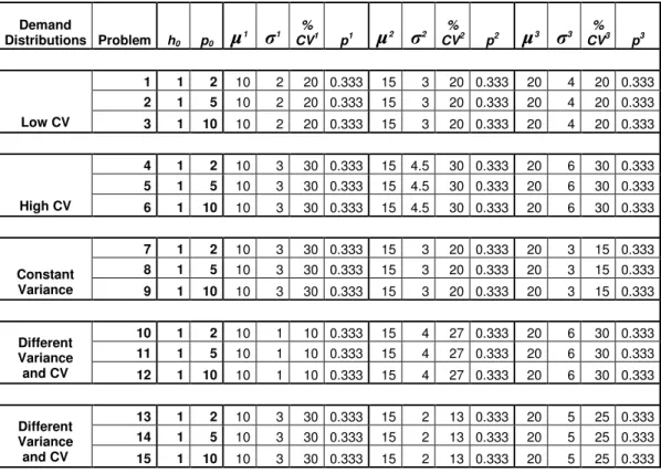
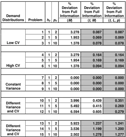
By search by numerical analysis, all three models will be tested on their capacity to converge to full information optimal costs. Before starting the numerical analysis, underlying inventory problem of the headquarters is defined with five different demand distribution settings. For each setting, ATM cash demand is generated by three different normal distributions with equal probability. Both the headquarters and branch know these three distributions whereas only branch knows which one of the three distributions generate the demand at each period. For each setting, three different unit stock-out costs for headquarters are used, making a total of 15 different inventory problems (Table 2). Each of these 15 inventory problems are solved by each model proposed in third section by numerical analysis. For

each model and problem, best external parameters that can be enforced to the branch by headquarters are searched by numerical procedures.

Demand Distributions Problem h0 p0 µ 1 σ1 % CV1 p1 _µ2 σ2 % CV2 p2 _µ3 σ3 % CV3 p3 1 1 2 10 2 20 0.333 15 3 20 0.333 20 4 20 0.333 2 1 5 10 2 20 0.333 15 3 20 0.333 20 4 20 0.333 Low CV 3 1 10 10 2 20 0.333 15 3 20 0.333 20 4 20 0.333 4 1 2 10 3 30 0.333 15 4.5 30 0.333 20 6 30 0.333 5 1 5 10 3 30 0.333 15 4.5 30 0.333 20 6 30 0.333 High CV 6 1 10 10 3 30 0.333 15 4.5 30 0.333 20 6 30 0.333 7 1 2 10 3 30 0.333 15 3 20 0.333 20 3 15 0.333 8 1 5 10 3 30 0.333 15 3 20 0.333 20 3 15 0.333 Constant Variance 9 1 10 10 3 30 0.333 15 3 20 0.333 20 3 15 0.333 10 1 2 10 1 10 0.333 15 4 27 0.333 20 6 30 0.333 11 1 5 10 1 10 0.333 15 4 27 0.333 20 6 30 0.333 Different Variance and CV 12 1 10 10 1 10 0.333 15 4 27 0.333 20 6 30 0.333 13 1 2 10 3 30 0.333 15 2 13 0.333 20 5 25 0.333 14 1 5 10 3 30 0.333 15 2 13 0.333 20 5 25 0.333 Different Variance and CV 15 1 10 10 3 30 0.333 15 2 13 0.333 20 5 25 0.333

Table 2: Problem Settings for Numerical Analysis

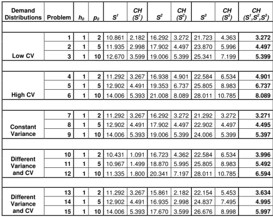
Before numerical analysis, optimum loading amounts for each demand scenario and full information optimal costs for the headquarters are calculated (Table 3). As mentioned before, optimum loading amounts are calculated assuming that headquarters knows which one of the three distributions generate the demand at each period. The first order condition derived at the beginning of chapter 3 is used for calculation of optimum

loading amounts S k*_{for all D} k

After, obtaining full information optimum solutions, numerical solutions for the problems are searched with three models of incomplete information. (M) policy was classical inventory model with lump-sum cost applied at the end of period, the second was (t, M) policy with lump-sum cost applied at time t within the period and the last was (t, L, p) policy with unit stock-out cost applied at time t within the period.

Demand Distributions Problem h0 p0 S1 CH (S1) S2 CH (S2) S3 CH (S3) CH (S1,S2,S3) 1 1 2 10.861 2.182 16.292 3.272 21.723 4.363 3.272 2 1 5 11.935 2.998 17.902 4.497 23.870 5.996 4.497 Low CV 3 1 10 12.670 3.599 19.006 5.399 25.341 7.199 5.399 4 1 2 11.292 3.267 16.938 4.901 22.584 6.534 4.901 5 1 5 12.902 4.491 19.353 6.737 25.805 8.983 6.737 High CV 6 1 10 14.006 5.393 21.008 8.089 28.011 10.785 8.089 7 1 2 11.292 3.267 16.292 3.272 21.292 3.272 3.271 8 1 5 12.902 4.491 17.902 4.497 22.902 4.497 4.495 Constant Variance 9 1 10 14.006 5.393 19.006 5.399 24.006 5.399 5.397 10 1 2 10.431 1.091 16.723 4.362 22.584 6.534 3.996 11 1 5 10.967 1.499 18.870 5.995 25.805 8.983 5.492 Different Variance and CV 12 1 10 11.335 1.800 20.341 7.197 28.011 10.785 6.594 13 1 2 11.292 3.267 15.861 2.182 22.154 5.453 3.634 14 1 5 12.902 4.491 16.935 2.998 24.837 7.495 4.995 Different Variance and CV 15 1 10 14.006 5.393 17.670 3.599 26.676 8.998 5.997

Table 3: Full Information Solution for Headquarters

4.1 (M) Inventory Policy

This model applies the lump-sum stock-out cost at the end of the period.

For each pair (h, M), the branch will find its optimal S1

amounts. According to these loading amounts expected cost for

headquarters CH(S1

, S2, S3) will be calculated for each pair (h, M). The numerical analysis needs a large enumeration not to miss the best solution. To simplify the enumeration process, for the analysis h is selected to be 1 and best M is searched as the solution depends on the ratio h/M. For the numerical analysis, the commercial Maple (http://www.maplesoft.com/products/Maple/features/index.aspx) program is used. The cost equations for both headquarters and branch are written using the normal distribution density functions. The optimization for the branch is done directly by the algorithm for a given M. According to these loading values the algorithm calculates expected cost for the headquarters. A complete search for M is done by iterations; at the beginning, big increment with a larger search scale is used. Then the search area is tightened and increment is decreased to 0.1. Increment is also decreased to 0.01 to search the ±0.1 neighborhood of the best M solution; but the solution did not improve further. Convexity of headquarters’ cost function with respect to lump-sum cost M is observed for each problem setting.

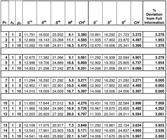
Results for each M is tabulated in to select the minimum cost CHb _and

corresponding Mb

, S1b, S2b, S3b values. For each one of the 15 inventory problem settings, selected optimal solutions are given in Table 4.

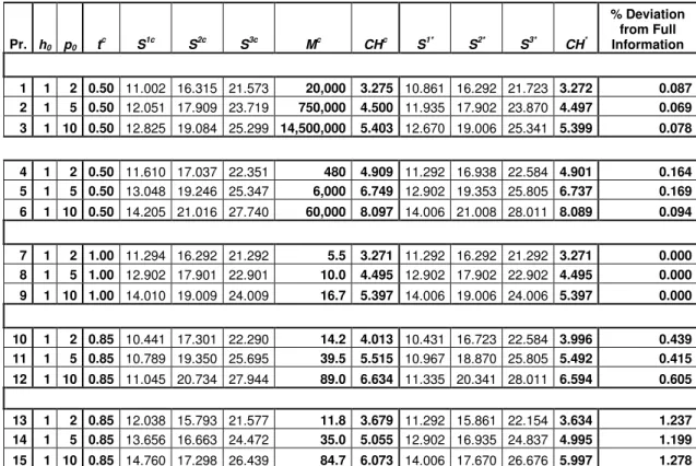
Except the settings with constant variance, the expected costs of solutions with (M) policy deviated more than 1 percent from the full information case. With the settings of different variance and %CV, deviations increased reaching to 7 percent for problem 10. Such high deviations encourage improvement for the inventory policy.

Pr. h0 p0 S1b S2b S3b Mb CHb S1* S2* S3* CH* % Deviation from Full Information 1 1 2 11.791 16.602 20.932 6.1 3.380 10.861 16.292 21.723 3.272 3.278 2 1 5 12.669 18.143 23.268 11.1 4.585 11.935 17.902 23.870 4.497 1.953 3 1 10 13.282 19.188 24.811 18.3 5.473 12.670 19.006 25.341 5.399 1.378 4 1 2 12.675 17.382 21.366 9.1 5.061 11.292 16.938 22.584 4.901 3.279 5 1 5 13.998 19.706 24.889 16.6 6.869 12.902 19.353 25.805 6.737 1.954 6 1 10 14.933 21.298 27.242 27.5 8.201 14.006 21.008 28.011 8.089 1.378 7 1 2 11.294 16.292 21.292 5.5 3.271 11.292 16.292 21.292 3.271 0.000 8 1 5 12.902 17.901 22.901 10.0 4.495 12.902 17.902 22.902 4.495 0.000 9 1 10 14.010 19.009 24.009 16.7 5.397 14.006 19.006 24.006 5.397 0.000 10 1 2 11.650 17.644 21.512 9.3 4.276 10.431 16.723 22.584 3.996 7.009 11 1 5 11.966 19.584 24.980 16.9 5.726 10.967 18.870 25.805 5.492 4.262 12 1 10 12.203 20.929 27.302 28.0 6.797 11.335 20.341 28.011 6.594 3.081 13 1 2 12.108 17.075 20.917 7.3 3.849 11.292 15.861 22.154 3.634 5.923 14 1 5 13.543 17.901 23.903 13.3 5.171 12.902 16.935 24.837 4.995 3.536 15 1 10 14.541 18.493 25.892 22.1 6.147 14.006 17.670 26.676 5.997 2.502

Table 4: Optimum Solutions for (M) Inventory Policy

4.2 (t, M) Inventory Policy

This model applies the lump-sum stock-out cost at time t between [0,1] within the period. For each triple (t, h, M), the branch will find its optimal

S1, S2, S3loading amounts. According to these loading amounts expected

cost for headquarters CH(S1

, S2, S3) will be calculated for each triple (t, h, M). To simplify the enumeration process, for the analysis h is selected to be 1 and best M is searched as the solution depends on the ratio h/M for each t. A complete search for t and M is done by iterations. The numerical analysis needs a very large enumeration due to high