Predicting crisis : this time is different (?)

PREDICTING CRISIS: THIS TIME IS

DIFFERENT (?)

˙Ihsan Do˘gramacı Bilkent University Ankara

PREDICTING CRISIS: THIS TIME IS

DIFFERENT (?)

Graduate School of Economics and Social Sciences of

˙Ihsan Do˘gramacı Bilkent University

A Master’s Thesis by

TU ˘

GBA SA ˘

GLAMDEM˙IR

In Partial Fulfillment of the Requirements For the Degree of

MASTER OF ARTS in

THE DEPARTMENT OF ECONOMICS

˙IHSAN DO ˘GRAMACI BILKENT UNIVERSITY ANKARA

I certify that I have read this thesis and have found that it is fully adequate, in scope and in quality, as a thesis for the degree of Master of Arts in Economics.

——————————————————– Assoc. Prof. Dr. Selin Sayek B¨oke

Supervisor

I certify that I have read this thesis and have found that it is fully adequate, in scope and in quality, as a thesis for the degree of Master of Arts in Economics.

—————————————————– Assoc. Prof. Dr. Fatma Ta¸skın

Second Reader

I certify that I have read this thesis and have found that it is fully adequate, in scope and in quality, as a thesis for the degree of Master of Arts in Economics. ——————————————

Assoc. Prof. Dr. Levent Akdeniz Examining Committee Member

Approval of the Graduate School of Economics and Social Sciences

————————— Prof. Dr. Erdal Erel Director

ABSTRACT

PREDICTING CRISIS: THIS TIME IS

DIFFERENT (?)

SA ˘GLAMDEM˙IR, Tu˘gba M.A., Department of Economics

Supervisor: Assoc. Prof. Dr. Selin Sayek B¨oke September 2012

This thesis aims to predict the currency, banking and debt crises and more specifically investigates the effect of the housing sector on the crisis prediction. This study is not only constructing a crisis prediction method, which uses the previous literatures data set, but also proposing a new one including the housing market data, and comparing the performances of the two in order to measure the impact of the housing market on the prediction power. The data are taken from World Bank, IMF, OECD and Eurostat and cover the years between 1999 and 2010. Multinomial logistic regression is used for crisis prediction. As an advantage, it prevents the ‘post-crisis bias’ problem; by this way the robustness of the analysis is also improved. The multinomial logistic regression is run for two different time windows ‘t-1, t, t+1’ and ‘t, t+1, t+2’ as t denoting the current year. By inclusion of the housing market data, the prediction power is increased from 60% to 100% in the case of ‘t-1, t, t+1’. The model sends no false alarms in this case. For the case of ‘t, t+1, t+2’, the in-sample prediction power is improved from 68% to 95% and the false alarm ratio is reduced from 6.6% to 3%. The-out-of-sample predictive performance of the system in ‘t, t+1, t+2’ is improved from 33% to 60% by the inclusion of the housing market data. Due to the restrictions of the data set, out-of-sample analysis could not be performed for the case of ‘t-1, t, t+1’. The proposed crisis prediction method succeeds in predicting

the crises of 2000s by using housing sector data. The impact of the housing sector in predicting crisis is clearly shown. Also, it is shown that chosen time window for the multinomial logistic regression in predicting crisis can lead to variations on the predicted results.

Key words: Predicting crisis, Currency Crisis, Banking Crisis, Debt Crisis, Post-crisis bias, Multinomial Logistic Regression, The Housing Market

¨

OZET

KR˙IZ TAHM˙INLEME: BU DEFA FARKLI (?)

SA ˘GLAMDEM˙IR, Tu˘gba Y¨uksek Lisans, Ekonomi B¨ol¨um¨u Tez Y¨oneticisi: Do¸c. Dr. Selin Sayek B¨oke

Eyl¨ul 2012

Bu tez ¸calı¸sması, para, bankacılık ve bor¸c krizlerini tahminlemeyi ve daha ¨

ozelde, konut piyasası verilerinin kriz tahminleme ¨uzerindeki etkilerini ara¸stırmayı ama¸clamaktadır. Bu ¸calı¸sma, sadece ge¸cmi¸s ¸calı¸smalarda kullanılan verilerden olu¸san bir kriz tahminleme metodu kurgulamamakta, aynı zamanda konut piyasası veri-lerinin kriz tahminlemedeki etkilerini ara¸stırmak i¸cin bunları da i¸ceren yeni bir kriz tahminleme metodu da ¨onermektedir. C¸ alı¸smada kullanılan veriler, D¨unya Bankası, Uluslararası Para Fonu (IMF), Ekonomik Kalkınma ve ˙I¸sbirli˘gi ¨Org¨ut¨u (OECD) ve Eurostat veritabanlarından alınmı¸stır ve 1999 - 2010 yillarıarasını kapsamaktadır. Kriz tahminlemede ‘C¸ ok Terimli Lojistik Regresyon’ tekni˘gi kullanılmı¸stır. Bir avantaj olarak, bu y¨ontem, ”kriz sonrasi sapma” problemini ¨onlemektedir. Analizin sa˘glamlı˘gı, bu ¸sekilde geli¸stirilmektedir. Regresyon analizi, t’nin ¸simdiki yılı be-lirtti˘gi durumda, ‘t-1, t, t+1’ ve ‘t, t+1, t+2’ ¸seklinde iki farklı zaman penceresi i¸cin ko¸sturulmu¸stur. Konut piyasası verilerinin eklenmesiyle, ‘t-1, t, t+1’ penceresindeki tahminleme g¨uc¨u %60’tan %100’e y¨ukseltilmi¸stir. Bu durumda, sistem herhangi bir yanlı¸s uyarı vermemektedir. ‘t, t+1, t+2’ penceresi i¸cinse, sistemin ¨orneklem i¸ci tahminleme g¨uc¨u %68’den %95’e ¸cıkarılmı¸s ve yanlı¸s uyarı oranı %6.6’dan %3’e d¨u¸s¨ur¨ulm¨u¸st¨ur. ‘t, t+1, t+2’ penceresi i¸cin, sistemin ¨orneklem dı¸sı tahminleme g¨uc¨u konut piyasası verilerinin dahil edilmesiyle, %33’ten %60’a y¨ukseltilmi¸stir. Veri k¨umesindeki bazı kısıtlamalar nedeniyle, ‘t-1, t, t+1’ penceresi i¸cin ¨orneklem dı¸sı

performans analizi yapılamamı¸stır. ¨Onerilen kriz tahminleme metodu, konut piyasası verileri ile 2000’li yıllardaki krizleri tahminlemeyi ba¸sarmı¸stır. Konut piyasası ver-ilerinin kriz tahminlemedeki etkisi a¸cık ¸sekilde g¨osterilmi¸stir. Ayrıca, ¸cok terimli regresyon analizi ile kriz tahminlemesi yapılırken, se¸cilen zaman pencerelerinin tah-minleme sonu¸clarında de˘gi¸sikliklere neden olabilece˘gi de g¨osterilmi¸stir.

Anahtar Kelimeler: Kriz tahminleme, Para Krizleri, Bankacılık Krizleri, Bor¸c Krizleri, Kriz Sonrası Sapma, C¸ ok Terimli Regresyon, Konut Sekt¨or¨u

ACKNOWLEDGEMENTS

I would like to express my sincere gratitude to my advisor Selin Sayek B¨oke for her supervision and invaluable guidance. I will always be indebted to her for her continuous support, patience and encouragement during my studies.

I also would like to thank to Refet G¨urkaynak for his continuous support and encouragement throughout my graduate study.

I am grateful to my examining committee members, Fatma Ta¸skın and Levent Akdeniz for their helpful comments and suggestions. Also, I would like to thank Erin¸c Yeldan and C¸ a˘grıSa˘glam for their helpful comments and suggestions during my graduate study.

I would like to thank to Bilkent University and TUBITAK for their financial support.

I owe my special thanks to my family for their unconditional love, support, pa-tience and encouragement throughout my life.

I am thankful to the big brothers: M. Orkun Sa˘glamdemir and ¨Omer Yetik for their patience, understanding and support throughout my study. It is very pleasing to know that, it is independent from where I am, I will never walk alone.

I am thankful to ¨Ozge Filiz Ya˘gcıba¸sı, for being my fellow who shows me that distance becomes meaningless when her friendship is the matter, it is a chance to have a sister like her.

I am thankful to Fulya ¨Ozcan and Se¸cil Yıldırım not only for sharing the time of my graduate study, but also for their friendship, which will last forever. They are one of the most important gains of this graduate study.

Last, but not least, I would like to thank to Maria Nawandish and C¸ i˘gdem Akbulut for their friendships and continuous support.

TABLE OF CONTENTS

LIST OF FIGURES . . . xii

CHAPTER 1: INTRODUCTION . . . 1

CHAPTER 2: LITERATURE SURVEY . . . 6

CHAPTER 3: THE HOUSING MARKET . . . 11

CHAPTER 4: DEFINITIONS, DATA AND METHODOLOGY . . 13

4.1 Definitions and Data . . . 13

4.2 Methodology . . . 20

CHAPTER 5: ANALYSIS . . . 26

5.1 Event Study Analysis . . . 26

5.2 Empirical Analysis . . . 43

5.2.2 Empirical results for the time window: ‘t, t+1, t+2’ . . . 55

CHAPTER 6: CONCLUSION . . . 66

BIBLIOGRAPHY . . . 70

APPENDIX A: FURTHER DETAILS . . . 76

LIST OF TABLES

4.1 Data set classified according to categories . . . 15 4.2 Countries used as data source . . . 17 5.1 Regime definition for the multinomial logit model for t-1, t, t+1 . . . 46 5.2 Results of the multinomial logit regression for t-1, t, t+1 . . . 48 5.3 Performance of the model without housing data for t-1, t, t+1 . . . . 52 5.4 Performance of the model with housing data for t-1, t, t+1 . . . 53 5.5 Crises correctly called with the model with housing data, t-1, t, t+1 . 54 5.6 Performance of the model without housing data on the reduced data

set for t-1, t, t+1 . . . 55 5.7 Regime definition for the multinomial logit model for t, t+1, t+2 . . 55 5.8 Results of the multinomial logit regression for t, t+1, t+2 . . . 57 5.9 Performance of the model without housing data for t, t+1, t+2 . . . 61 5.10 Performance of the model with housing data for t, t+1, t+2 . . . 62 5.11 Crises correctly called with the model with housing data, t, t+1, t+2 63 5.12 Performance of the model without housing data on the reduced data

set for t, t+1, t+2 . . . 64 A.1 Data set classified according to source . . . 76

LIST OF FIGURES

1.1 Housing Prices for some developed countries . . . 3

5.1 Event Study Analysis for time window ‘t-1, t, t+1’ - I . . . 31

5.2 Event Study Analysis for time window ‘t-1, t, t+1’ - II . . . 32

5.3 Event Study Analysis for time window ‘t-1, t, t+1’ - III . . . 33

5.4 Event Study Analysis for time window ‘t, t+1, t+2’ - I . . . 39

5.5 Event Study Analysis for time window ‘t, t+1, t+2’ - II . . . 40

5.6 Event Study Analysis for time window ‘t, t+1, t+2’ - III . . . 41

CHAPTER 1

INTRODUCTION

This hypothesis of this study is formed on the supposed impact of the housing sector on predicting crisis. This question is valuable for the following reasons: Crises are events that have been re-occurring since the 14th _{century and policy makers could}

not prevent outbreak of crises from that time. This is why crisis prediction is crucial for the whole economy. In this study, the housing sector is analyzed as an important indicator for predicting crisis; since most of the crises seem to have the common characteristics of having started in the housing markets. Due to all these reasons above, the housing market implication on predicting crisis will analyzed in this thesis. Economic crisis, as being one of the common problems of the world, has a history that dates back to 14th _{century in England [Reinhart and Rogoff(2008b)]. Since the}

crisis creates a destructive impact on the economy, both policy makers and academics search for policies to avoid the crisis. If the economy consisted of mechanisms, which followed the same rules and did not change until the policy makers made any reg-ulations, they would achieve their aim. However, the reality is different. There are many actors in the system and each of them makes different contributions. Due to this fact, the measures, which are taken to avoid the crisis, do not work.

Once it is accepted that the economic crises are situations which the economies cannot escape from, the optimum solution turns out to become predicting the coming crisis before it hits the economy, in order to protect the whole economic system as much as possible. As a consequence, the requirement for predicting crisis before its outbreak arises.

There exist quite a large number of studies on predicting crisis in the literature. They generally use financial and macroeconomic data to predict crisis and work only on one type of crisis on its own. Some of them work on banking crises, some on currency crises, and some on debt crises. Only Babeck´y et al (2012) try to find the early warning indicators for currency, banking and debt crisis [Babeck´y(2012)]. However, none of the previous studies both try to predict all types of crises and use housing sector data among with the financial and macroeconomic variables except Rose et al (2011).

The previous studies generally emphasize the similar indicators, which come from macroeconomic and financial data. Also, more or less, they usually apply the same techniques, which are being used from the very beginning of the early warning system studies. Every analysis with the aim of constructing an early warning system is a step to achieve higher prediction power; however, since economy has a very dynamic structure, both the prediction techniques and the data to be used in the estimation process have to evolve through time to improve the ability of catching the alterations in the system. In that respect, importance of the housing market on economic crises is analyzed in this thesis, and an early warning system is constructed by taking the effects of the housing sector data into consideration.

In this thesis, all types of crisis (either currency, banking or debt) are aimed to be predicted by combining the indicators used in the previous studies in the literature with the housing sector variables. Since the housing sector is the common problematic part of the economy for the countries which have economic crises after 2000s, it is

worth to search for its impact on predicting crisis. Rose et al (2011) is the first study, which uses ‘percentage change in real estate prices’ as an indicator of housing market data in crisis prediction. Although the authors introduce the housing market data into the system, they fail to predict the crisis for 107 countries. As it is seen from the following figure, the housing prices followed upward trend for some developed countries such as Australia, Canada, United Kingdom and United States:

Figure 1.1: Housing Prices for some developed countries

In this study, the analysis on the crisis prediction is separated into two cases: In the first case, the crisis is predicted by running a multinomial logistic regression over a time window of ‘t-1, t, t+1’ where ‘t’ denotes the current year of investigation, ‘t-1’ is the year before the current one and ‘t+1’ is the year after it. Hence, given that a crisis has occurred at time t, then the behavior of the variables within t-1 to t+1 is analyzed. That is, the values both before and after the crisis are taken into consideration. In the second case, again the multinomial logistic regression technique is used. However, the time window is now changed to ‘t, t+1, t+2’. In this case,

the analyzed time window covers the current year and two consecutive years after it. Hence, the behavior of the variables before the crisis is not taken into consideration but the focus is on their current and future values.

For both time windows of multinomial logistic regression, the estimation is con-structed from two different stages. In the first stage, the variables which are used in the prior crisis prediction studies are used in the multinomial logistic regressions for both time windows to show the prediction powers of these variables in predicting the crises that arose after 2000s. Then, in the second stage these prior studies’ variables are combined with the housing market data set, which indicates the effects of housing sector. This combined data set is used in the multinomial logistic regressions for both time windows to show the prediction powers of these variables. By comparing the results of first and second stage analyses, it is possible to see the difference, which arises due the inclusion of the housing sector data.

In this thesis, the following questions are answered: Do housing market data make any improvements in predicting crisis? Does the prediction power differ depending on the time window of the multinomial logistic regression? Which time window is more suitable to be used in crisis prediction to attain a higher prediction power?

Applying the procedure described above, the empirical results show that the hous-ing sector data, make an improvement in predicthous-ing crisis. The prediction power changes depending on the time window of the multinomial logistic regression. On the other hand, since the publicly available housing data set is restricted, it does not allow to make an out-of-sample performance analysis for the time window of ‘t-1, t, t+1’. Consequently, it is not possible to make a comparison between the crisis prediction powers of the two different time windows.

This thesis is organized as follows: Chapter 2 analyzes the literature. Chapter 3 explains the importance and impact of the housing market on the economy. Chapter

4 gives details on the data and the methodology. Chapter 5 reviews the event study and empirical analysis results. Chapter 6 concludes.

CHAPTER 2

LITERATURE SURVEY

The economy is a complete system, which consists of different dynamics. As the countries economies are getting integrated in terms of financial dependence on each other, the economic decisions which are taken by one country turns out to be an important indicator for all economies over the world. As a result of this, this system needs to be controlled in order to protect it against an outbreak of a crisis. The policy makers in each country try to control and arrange any variation for every indicator, which may affect the other components and cause the whole system to collapse, by utilizing the tools and mechanisms they have in hand.

Although there are many regulatory mechanisms, which arrange and supervise the system, unexpected changes still do appear. These changes sometimes become so uncontrollable that they drive the economy into crisis. These crises may be the result of some already existing dynamics or may arise due to a new dynamic, which has recently been introduced to the system and has become crucial in an ongoing basis on the economic conditions.

As a matter of fact, the economic crisis history is as old as the history of economy. Since there are many indicator factors constituting the whole economy - and new indicators get involved in this system continuously - it is impossible to think of an

economy, which never suffers from an economic crisis. On the other hand, the most appropriate solution for reducing the destructive impact of a crisis on the economy is to predict the coming of it and take the required precautions so as to protect the economy as much as possible. This indeed is the motivation behind designing an Early Warning System, aim of which is to predict a crisis before it hits the economy. There are different types of economic crises as currency crisis, banking crisis and debt crisis. The policy makers generally tried to construct Early Warning Systems for each type of crisis on its own. After mid 90s, the currency crisis turned out to become a common problem of the economic systems. This crisis type is analyzed by Kaminsky et al (1998) and in this analysis, a new non-parametric approach is constructed, which is also called as the signal approach [Kaminsky and Reinhart(1998)]. This approach is prominent in the field of early warning systems, whose prediction power is 70% in the in-sample analysis. By this study, it has been shown that it was possible to predict a crisis with a non-parametric approach. After this analysis, the early warning system literature has been introduced a new term as false signal, standing for the cases in which the system warns about a coming crisis but there is no upcoming crisis indeed. Then researchers sought for new estimation techniques to construct early warning systems. Berg et al (1999a) use the same data set and crisis definition as Kaminsky et al to work on the currency crisis [Berg and Pattillo(1999a)]. However, their estimation technique is the probit approach for designing the early warning system, where the dependent variable takes the value of one for the case of a coming crisis and zero for all other cases. The probit approach is more practical than the signal approach since it allows testing the statistical significance and coefficient constancy overtime and countries.

In addition to the probit approach Demirguc-Kunt et al (1997) introduce a new estimation tool [Demirguc-Kunt(1997)]. They try to find the main reason behind the

banking crisis by working on both developing and developed countries. They apply multivariate logit model to identify the determinants of the banking crisis.

Since the important thing is not only constructing the early warning system but also predicting the crisis with the highest success ratio, the literature seek for new techniques, new data sets and indicators to increase their prediction power. Binomial logit is another technique used but its results suffer from post-crisis bias which is described in Section 4.2.

Bussiere et al (2002) construct an early warning system aiming for predicting currency crisis by using the estimation technique of multinomial logistic regres-sion [Bussiere and Fratzscher(2002)]. Since they criticize the prediction power of the binomial logit model, their analysis consists of both binomial and multinomial logistic regression models. The data set they use contains 20 open economies and spans the years from 1993 to 2001. According to their estimations, the binomial logistic regression predicts the crisis entry periods with a success ratio of 56,9% and multinomial logistic regression estimates the same periods with 65,5% success. After their contribution, the multinomial logistic regression technique replaces the binomial logistic regression in the early warning system literature.

Although the early warning system techniques are generally parametric, there are some analyses, which compare the prediction power of the different methods such as the one done by Peltonen (2006) for predicting currency crisis [Peltonen(2006)]. In this study, two early warning systems are constructed by using two different ap-proaches: probit approach, which is parametric, and artificial neural network (ANN) model as a non-parametric approach. Their data set comprises eight exogenous indi-cators, and the time interval spans the period between 1980 and 2001 for 24 emerging economies. The main contribution of this paper is that, it compares the prediction power of the probit model with that of the Artificial Neural Network approach for in-sample and out-of-in-sample performance in predicting currency crisis. Then it is shown

that the ANN approach outperforms the probit model for predicting currency crisis regarding the in-sample performances, but both methods’ out-of-sample performances are weak.

Although most of the early warning systems are designed to predict the currency crisis, after 2000s, with the financial liberalization and globalization, the reason of the economic crises do change with the structure of the economy. As a consequence of this change, different types of crises emerge and attract the literature’s attention. Manasse et al (2003) constructed an early warning system with the aim of predicting debt crisis [Manasse and Roubini(2003)]. Their data set consists of 47 markets and the time interval spans years from 1970 to 2002. In this analysis, both a non-parametric approach - Classification and Regression Tree (CART) - and a parametric approach binomial logistic regression - are applied and their prediction powers are compared. According to the results, binomial logistic regression predicts 74% of the crises where CART predicts 89% of the crisis entries. On the other hand, CART sends more false alarms then the binomial logistic regression. No out-of-sample analyses are applied.

The debt crisis is analyzed by many other researchers such as Bruner et al (1987) and Roubini et al (2005). Roubini et al (2005) apply CART as well, using 47 countries’ data, which belongs to the period of 1970 to 2002 [Roubini(2005)]. 10 exogenous variables are used for the estimation process and the prediction power of this model is 85% for the in-sample performance and 35% for the out-of-sample performance.

To estimate the debt crises, more techniques and crisis definitions are used with the aim of increasing the estimation power. One of them is constructed by Ciarlone et al (2005) [Ciarlone and Trebeschi(2005)]. In this analysis, they use multinomial logistic regression to predict the crisis. Also, they run a binomial logistic regression to make a comparison between the estimation powers of these two models. By using 28 countries’ data, which also span the years from 1980 to 2002, they find that, with the binomial logistic regression’s in-sample prediction power of the model is 72,5%. For the same

data set, the in-sample prediction power increases to 76% with the multinomial logistic regression. They do not make an out-of-sample performance analysis for the models. One year later, again Ciarlone et al (2006) construct a new early warning system to predict debt crisis [Ciarlone and Trebeschi(2006)]. The debt crisis definition and multinomial logistic regression construction is different compared to their previous analysis. This analysis uses the same data set, but their prediction power is 78% for the in-sample performance and 70% for the out-of-sample performance.

Rose et al (2009, 2011) construct an early warning system, which uses multiple-indicators multiple-causes (MIMIC) model for the estimation for 107 countries, to predict the 2008 financial crisis [Rose(2009), Rose(2011)]. They analyze 60 potential causes of this crisis but they accept that their early warning system could not predict the crisis.

Although, Rose et al (2009, 2011) could not predict this type of crisis by using housing sector data, the searched hypothesis question of the impact of housing sector on predicting crisis is still important. As it will be argued in the following section, the indicators of the housing market are important on predicting crisis as crisis indicators.

CHAPTER 3

THE HOUSING MARKET

In this study, the housing sector is analyzed as a potential reason for the economic crisis and constitutes the most important part of the crisis prediction. There are lots of independent reasons denoting the importance of the housing sector, which led to the question of whether it could be a cause for the crisis or not and motivated this research.

Although the housing prices generally change with the overall price level in the economy, the situation is a little bit different compared to the usual behavior, as explained by Andre (2010) as follows: During the 2001 recession, house prices got disconnected from the business cycle. Low interest rates and mortgage innovations fueled housing demand, which in turn led to an expansion in the housing prices. This housing price expansion had three main aspects as: Real house price has soared, the expansion has been exceptionally long, most of the industrialized countries experi-enced house price boom simultaneously. In reaction to this rise in the housing prices, the residential investment increased [Andre(2010)].

Although the number of the houses increased, their price level did not show any reduction and this increased the house owners’ wealth. The level of wealth is a determinant factor of the consumption level for the overall economy, as shown by

Case et al (2001). Their study shows that, the changes in the national wealth are associated with the changes in consumption. In addition, they pointed out that, the tendency to consume out of stock market wealth is different from the tendency to consume out of housing wealth [Case(2001)]. The different impact of the housing wealth and stock market wealth on consumption is compared by Benjamin et al (2004) for the US economy. They reach the result that, the decline in the stock market during 2000 and 2001 had a limited impact on aggregate demand because of an offsetting real estate wealth effect [Benjamin(2004)].

Goodhart et al (2008) accept the link between aggregate consumption and hous-ing sector as a determinhous-ing factor for monetary variables and macroeconomics. They found out that, there is a multidirectional link between house prices, monetary vari-ables and the macro economy. Moreover, this link between house prices and monetary variables is found to be stronger over a more recent sub-sample from 1985 till 2006. The housing boom is not only important for the housing sector itself but it also affects the financial sector, monetary sector and credit sector [Goodhart(2008)].

Furthermore, the real estate boom is accepted as a source of fragility by Buiter et al (2009) since it channeled investment away from more productive areas into unproductive residential construction [Buiter(2009)].

This framework forms the basis of my thesis. It suggests that housing market developments influence crisis. This also forms the basis for the analysis by Rose et al (2009, 2011). But they could not predict crisis [Rose(2011)].

Although the importance of the housing sector is pointed out by many studies in the literature, the impact of this sector on the crisis has not been shown. Hence, the aim of this study is to analyze the effects of the housing sector on the occurrence of economic crisis, and it is expected to find an improvement to the prediction power of the early warning systems by using the housing sector data.

CHAPTER 4

DEFINITIONS, DATA AND

METHODOLOGY

4.1

Definitions and Data

In predicting crisis, there are many important steps in the construction part and the first one of them is defining the crisis conditions. The next step after categorizing the conditions is the prediction of the coming of a crisis. At this point, the most important thing is choosing the right indicator variables. The main goal of crisis prediction is to construct a model, which is capable of catching upcoming crises with the minimum possible number of misses. Therefore, the system needs some precise threshold, which helps in charting out. There are some basic questions answers of which help in leading the variation of the model. These questions are as follows:

• What is the definition of the crisis?

• Which countries constitute the research area?

By answering these questions, the general outline will be designed and then it will be easy to construct the model by using these answers. Basically, there are three kinds of economic crises as banking crisis, currency crisis and debt crisis. They differ from each other in terms of some basic causes and results but their general effect is the same: lowering nations’ welfare. Motivated by this fact, the system proposed in this study aimed to predict all these three types of crises. A brief definition for each type of crisis can be given as follows [Reinhart and Rogoff Online Resources]:

• Currency crisis: The economic situation is defined to be a currency crisis if the annual inflation rate is 20 percent or higher and the annual depreciation versus the United States dollar is 15 percent or more.

• Banking Crisis: If one or both of the following two conditions hold, the econ-omy is said to have a banking crisis:

(i) Bank runs that lead to the closure, merging or takeover by the public sector of one or more financial institutions.

(ii) If there are no runs, the closure, merging, takeover or large scale government assistance of an important financial institution (or group of institutions) that marks the start of similar outcomes for other financial institutions.

• Debt Crisis: It is identified in the case of a failure to meet a principal or interest payment on the due date (or within the specified grace period). The episodes also include instances where rescheduled debt is ultimately extinguished in terms less favorable than the original obligation. In addition to this condition, the situations of banks being forced to freeze their deposits or forcible conversions of such deposits from dollar to local currency are considered to be debt crisis conditions as well. These conditions for different types of crises cases have been defined in accordance with the previous studies of Reinhart and Rogoff to identify currency, banking and debt crises [Reinhart and Rogoff Online Resources].

The data set is formed from 111 exogenous variables, which is mainly divided into two main branches. The first group represents the prior studies variables, which were collected to predict currency, banking and debt crises. The second part of the data set consists of housing market data. This second group of variables has not been used in the prediction of the crises until now. The overall data set classified according to their categories are given in the following table:

Table 4.1: Data set classified according to categories Source Set of Variables

Capital Account Net open position in the foreign exchange to capital ratio, FDI, total reserve growth, FDI to GDP

Debt Profile Household debt to GDP, short term debt to international reserves, domestic credit to private sector, interest payment on total external debt, total external debt stocks, short term external debt stocks, short term debt to total reserves, short term debt to total external debt , interest payments on short term external debt, central govern-ment debt as percentage of GDP, private non-guaranteed external debt stocks, public and publicly guaranteed external debt stocks, bank non-performing loans to total gross loans, total debt service percent of exports, interest payments on long term external debt, total external debt to GDP, external debt to exports, international reserve to total external debt, short term debt to GDP, total external debt to total reserves, short term debt international reserve growth, real domestic credit growth, interest payments on external debt to international reserve, interest payment on short term debt to GDP Current Account Exchange rate, export, import, current account balance, export

growth rate, import growth, current account to GDP, Deviations of real exchange rate from trend

International Variables

Foreign exchange reserves, use of IMF credit, portfolio equity net inflows, net ODA received

Financial Liberalization

Deposit rate, bank liquid reserve to bank asset ratio, domestic credit provided by banking sector percent of GDP, deposit insurance, terest rate spread, risk premium on lending, S&P global equity in-dices (annual percentage change), stocks traded (total value), stocks traded turnover ratio, international reserve growth

Source Set of Variables Other Financial

Variables

Money supply, return on equity, liquid asset to total asset, treasury bill rate, liquid asset to short term liabilities, non performing loans to total gross loans, return on asset, sectoral distribution of total loans(deposit takers), sectoral distribution of total loans(residents), bank capital to asset ratio, inflation volatility, change in terms of trade, the ratio of M2 reserve to international reserve

Real Sector Industrial production, GDP, unemployment rate, GDP growth, trade in services percent of GDP, real interest rate, inflation, GDP per capita, gross saving percent of GDP

Institutional variables

Capital adequacy ratio, degree of openness to international trade, financial requirement to total reserve

Fiscal Variables Short term interest rates of government securities and government bonds, medium- log term government securities and government bonds, government revenue excluding grants percent of GDP, gov-ernment expense percent of GDP, tax revenue percent of GDP, fiscal surplus to GDP

Housing Sector Residential real estate prices, residential real estate loans to total loans, commercial real estate loans to total loans, house prices per-centage change over previous period, house price ratio to rent ratio, house price to income ratio, household wealth and indebtedness as a percentage of nominal disposable income, housing expense in per-cent of GDP, building permits, gross residential loans, house price percentage change, housing completions, housing starts, net residen-tial loans, nominal house price indices (2000=100), nominal house prices annual percentage change, number of housing transactions, real gross fixed investment in housing annual change, representative interest rates on new mortgage loans, residential mortgage debt to GDP ratio, total dwelling stock, total outstanding residential loans, rate of change of housing price to GDP growth, the ratio of real gross fixed investment in housing annual change to GDP growth, the ratio of representative interest rate on new mortgage loans to real interest rate

Table 4.2: Countries used as data source Countries

Austria, Cyprus, Czech Republic, Denmark, Estonia, Finland, France, Germany, Greece, Hungary, Ireland, Italy, Latvia, Lithuania, Luxembourg, Netherlands, Poland, Portugal, Romania, Slovakia, Spain, Sweden, United Kingdom, Iceland, Nor-way, Russia, Turkey, Ukraine and United States

While grouping the above variables, the categorization is done according to prior studies [Kaminsky and Reinhart(1998)].This data set includes the period between 1999 and 2010 for the countries given in Table A.1:

Housing sector and its components are among those factors, weights of which started overriding the effects of other variables in causing crises after 90s. Also their impact on the economy gradually increase [Goodhart(2008)]. Since the aim is con-structing a framework to study the role of the housing market, which is capable of predicting different crisis, related factors identified by previous studies plus housing market data will be included in the analysis.

Multinomial logit regression is the methodology, which is used in constructing the crisis prediction framework. In this model, the system needs to use sufficiently enough data to make prediction.

As mentioned above, with the inclusion of housing variables, the analysis narrows down in terms of both the countries and time interval in both cases of time windows used (‘t-1, t, t+1’ case and ‘t, t+1, t+2’ case). The number of observations used in the analysis decreased from 1942 observations to 362 observations for ‘t-1, t, t+1’ case and to 332 observations in ‘t, t+1, t+2’ case when housing market indicators are added into the analysis.

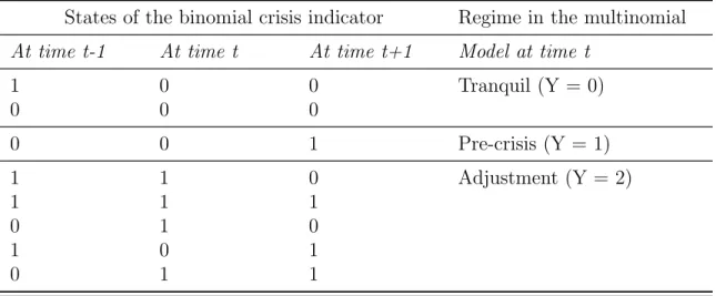
The dependent variable of the regression indicates the state of the economy iden-tified for three different cases as pre-crisis, crisis and tranquil periods. The dependent variable is generated over a crisis indicator variable, which takes the value of 1 for

the years with crises and value of 0 otherwise. (The details of the construction of time windows and the dependent variables are given in Section 5.2). These peri-ods of crisis, pre-crisis and tranquility are created in accordance with the previous studies in the crisis predicting literature [Glick(1999), Manasse(2009), Laeven(2008), Reinhart and Rogoff Online Resources].

While running the estimations, the approach proposed by Ciarlone et al (2005, 2006) is followed. In the first step separate multinomial logistic regres-sions have been run for each single variable on its own to check their statistical significance. The main estimation is run by only including those, which were proven to be significant at this first stage. In the estimation, some groups of these variables had exhibited similar properties in terms of their effects on the economy. As a result of these similarities, it was possible to create some sub-groups from these variables in accordance with the prior studies for currency, banking and debt crises [Berg and Pattillo(1999b), Bussiere and Fratzscher(2002), Kaminsky and Reinhart(1998), Demirguc-Kunt(1997), Manasse and Roubini(2003), Ciarlone and Trebeschi(2005), Ciarlone and Trebeschi(2006)].

After these groups were constructed, the multinomial logit regressions were run for each group for predicting crises. After this, for every group top three best performers, showing the highest variation passing through from tranquil period to pre- crisis period in terms of odds ratio, were selected for the next step. For some of these groups, the mlogit regression could not converge to a solution because of either insufficient number of observations or concavity problems. Such groups have been further divided into smaller sub-groups until a successful mlogit run could be achieved. This method of creating groups and selecting best performers for the next step continued up until reaching the final working combination of variables whose odds ratios showed the highest deviation while passing from tranquil period into the pre-crisis period with in 95% confidence interval.

Finally, all sub-groups’ best performers were put together to create the set of main independent variables to be used in the model for predicting crisis. In the analysis part the prediction was done according to two different time windows as ‘t-1, t, t+1’ and ‘t, t+1, t+2’ where t denotes the current year of concern. Since the estimation of these two models depended on different time windows, the independent variables, which were used in these models, are not same.

The final group, which is used in the case of time window ‘t-1, t, t+1’ consists of the following variables: The ratio of FDI to GDP, total reserve growth, the ratio of domestic credit to private sector (% of GDP), trade in services (% of GDP), the ratio of domestic credit provided by banking sector (% of GDP), export growth, GDP growth, real domestic credit growth, bank capital to asset ratio, S&P global equity indices (annual % change), tax revenue (% of GDP), real interest rate, deposit rate, interest rate spread, representative interest rate on new mortgage loans, total outstanding residential loans, net residential loans.

The final group, which is used in the case of time window ‘t, t+1, t+2’ is formed from the following variables: International reserve growth, the ratio of current account to GDP, total reserve growth, the ratio of FDI to GDP, change in terms of trade, domestic credit to private sector (% of GDP), domestic credit provided by banking sector (% of GDP), real domestic credit growth, import growth rate, degree of open-ness, export growth rate, S&P global equity indices (annual % change), tax revenue (% of GDP) , bank capital to asset ratio, interest rate of government securities & government bonds, bank liquid reserves to bank asset ratio, central government total debt (% of GDP), residential mortgage debt to GDP ratio, real gross fixed investment in housing annual change, total dwelling stock, housing completions, representative interest rate on new mortgage loans, nominal house prices annual percentage change, change of housing price to GDP growth.

4.2

Methodology

There are different kinds of estimation techniques in the early warning systems. These techniques are divided into two main groups as parametric and non-parametric tech-niques. Since the variables are assumed to be statistically independent, using a para-metric estimation method is much more suitable for constructing an early warning system.

Logistic regression is one of the parametric techniques, which has many advantages as follows:

• Logistic regression allows properties of a linear regression model to be exploited. • The logistic regression value can vary between −∞ and +∞. Although, the model coefficients’ value change −∞ and +∞, the probability remains 0 and 1, by this way it gets easy to make interpretation and analysis depending on the data.

• The logit model can directly affect the odds ratio, as an advantage of this property, the changes in the model can be totally reflected to the ra-tio [Online Resources PennState University].

Logistic regression has two branches as binomial logistic regression and multi-nomial logistic regression. Bimulti-nomial regression function analyzes the economy by separating it into crisis and adjustment periods. This method has been used in many studies to predict crisis [Ciarlone and Trebeschi(2005), Manasse and Roubini(2003), Davis and Karim(2008b)]. Although the models in these papers predicted many crises, they were ridden by the post crisis bias.

Post-crisis bias means that, while predicting a crisis, the independent variables are analyzed depending on their values during and directly after a crisis. However, the aim for constructing early warning systems is predicting crises before they hit

the economy. The most suitable way of doing this is comparing the variation of the variables before a crisis compared to their values during tranquil periods, when their values are sustainable. But a binomial logit model compares the pre-crisis observation with that in both the tranquil periods and crisis/adjustment periods. That is, the binomial logit model does not differentiate the tranquil period from an adjustment period. This induces an important bias, as the variation of the independent variables is very different during tranquil times as compared to crisis/recovery period.

There are two ways to overcome this post-crisis bias. The first one is dropping all crisis/adjustment observations from the model and the second way is using a dis-crete dependent variable, which gives more than two outcomes: multinomial logistic regression [Bussiere and Fratzscher(2002)].

The setup of the multinomial regression model is the same as that in logistic regression; the key difference is that, the dependent variable of logistic regression is formed from two outcomes whereas the dependent variable of multinomial logistic regression consists of more than two possible outcomes.

In order to explain the logistic regression, logistic function has to be introduced as: π(x) = e (β0+β1X1+e) e(β0+β1X1+e)_{+ 1} = 1 e−(β0+β1X1+e)_{+ 1}, (4.1) g(x) = ln π(x) 1 − π(x) = β0 + β1X1+ e, (4.2) π(x)/1 − π(x) = eβ0+β1X1+e _(4.3)

The logistic function takes values from negative infinity to positive infinity and the output value changes between 0 and 1.

In these equations, g(x) represents the logit function of given predictor X. ln present the natural logarithm, π(x) gives the probability of being in a case, β0 is

the intercept from the linear regression equation. β1X1 is the regression coefficient

multiplied by some value of the predictor, and base e means the exponential function. The e in the linear regression equation stands for the error term.

To apply a logistic regression model, a series of N observed data points is needed. Each data point i, consists of a set of M explanatory variables from x1,i to xM,i and

associated dependent variable Yi.

In this model, it is assumed that the dependent variable Y is a random variable distributed according to the Bernoulli distribution. Each outcome of the dependent variable is determined by an unobserved probability pi, which is special to the outcome

itself but also connected to the explanatory variables as well. The overall picture for the logistic regression can be explained by the following equations [Greene(2003)]:

Yi|x1,i, ..., xm,i ∼ Bernoulli(pi)

E[Yi|x1,i, ..., xm,i] = pi

P r(Yi|x1,i, ..., xm,i) =

       pi, if Yi = 1 1 − pi if Yi = 0

P r(Yi|x1,i, ..., xm,i) = pYii(1 − pi)(1−Yi)

(4.4)

The logistic regression can be designed by modeling the probability value of pi

using a linear predictor function. Hence, pi will be a linear combination of the

ex-planatory variables and a set of regression coefficients that are specific to the model. The predictor function f (i) for a data point i will be in the following form:

β0, ..., βM are the regression coefficients and each gives the relative impact of a

particular explanatory variable on the dependent variable. If,

• the regression coefficients β0, β1, ..., βk are grouped into a single vector β of size

k + 1;

• for each data point I, an additional explanatory variable x0,i is added, with a

fixed value of 1, similar to the intercept coefficient β0;

• the explanatory variables x0,i, x1,i, ..., xk,i are grouped into a single vector Xi of

size k + 1

then the linear predictor function turns into

f (i) = β.Xi (4.6)

The basic setup of the multinomial logistic regression is similar to that of the logis-tic regression. However, the dependent variable for a multinomial logislogis-tic regression is a categorical variable that is, it has more than two discrete possible outcomes. For multinomial logistic regression the probability of observation i having the outcome k is given by the linear predictor function f (k, i) as following:

f (k, i) = β0,k + β1,kx1,i+ β2,kx2,i+ ... + βM,kxM,i (4.7)

βm,k is the regression coefficient that relates the mthexplanatory variable with the

kth dependent variable outcome. As with the same in the logistic regression function,

the predictor function can be written as;

f (i) = βk.Xi (4.8)

βk is the set of regression coefficients related with outcome k and xi is the set

To clarify the multinomial logistic model, one can assume that the multinomial logistic regression for a dependent variable with K different possible outcomes is like running a series of K-1 independent binomial logistic regressions in which one outcome is chosen as the base and the rest K-1 outcomes are separately regressed relative to the base outcome. In the case of the last outcome K being selected as the base, the probabilities would be calculated as follows:

ln P r(Yi = 1) P r(Yi = K) = β1.Xi ln P r(Yi = 2) P r(Yi = K) = β2.Xi .... lnP r(Yi = K − 1) P r(Yi = K) = βK−1.Xi (4.9)

Separate set of regression coefficients are introduced, one for each possible out-come. After exponentiation of both sides of the equations and solving, the resulting probabilities would be:

P r(Yi = 1) = P r(Yi = K)eβ1.Xi

P r(Yi = 2) = P r(Yi = K)eβ2.Xi

....

P r(Yi = K − 1) = P r(Yi = K)eβK−1.Xi

(4.10)

Since the sum of the K probabilities is equal to 1, the probability of the base outcome will be:

P r(Yi = K) =

1 1 +PK−1

k=1 eβk.Xi

The rest of the probabilities can be found as follows: P r(Yi = 1) = eβ1.Xi 1 +PK−1 k=1 eβ 0 k.Xi P r(Yi = 2) = eβ2.Xi 1 +PK−1 k=1 eβ 0 k.Xi ... P r(Yi = K − 1) = eβK−1.Xi 1 +PK−1 k=1 e β_k0.Xi (4.12)

The multinomial logistic regression model has an important assumption, which is the independence of irrelevant alternatives. The independence of irrelevant alter-natives assumption states that, the odds of preferring one class to another do not depend on the presence or absence of other irrelevant alternatives. This condition makes it possible to model the choice of K alternatives as a set of K-1 independent binary choices, in which one alternative is chosen as the base outcome and the other K-1 alternatives are compared against it.

In this study, the dependent variable, Y, for the multinomial logit model has 3 different discrete outcomes as 0, 1 and 2 as 0 corresponding to tranquil period, 1 corresponding to the pre-crisis period and 2 corresponding to the state of being in crisis (may be mentioned adjustment period as well). In such a case, the calculated probabilities for the possible outcomes can be given as follows:

P r(Yi,t = 0) = 1 1 + eXi,tβ1 _{+ e}Xi,tβ2 P r(Yi,t = 1) = eXi,tβ1 1 + eXi,tβ1 + eXi,tβ2 P r(Yi,t = 2) = eXi,tβ2 1 + eXi,tβ1 _{+ e}Xi,tβ2 (4.13)

CHAPTER 5

ANALYSIS

5.1

Event Study Analysis

The analysis started with 111 exogenous variables and the number of variables decreased to 17 in the case of time window ‘t-1, t, t+1’ and to 24 in the case of time windows ‘t, t+1, t+2’ after a series of groupings and selecting the best three performers from all groups. The groupings have been done according to the related literature [Berg and Pattillo(1999b), Bussiere and Fratzscher(2002), Kaminsky and Reinhart(1998), Demirguc-Kunt(1997), Manasse and Roubini(2003), Ciarlone and Trebeschi(2005)]. Although, the literature was successful in predicting more than a half of the crises, it is still necessary to check the behavior of each exogenous variable before, during and after the crises periods in order to make sure that they are the indicator variables, variations of which signals the coming of a crisis.

By this analysis, the best performers’ behaviors, which are selected by the grouping procedure, are analyzed for a 7-year time interval. If the variables behave differently between the tranquil period and pre-crisis period, it will prove that the variables are suitable to use in predicting crisis. If they follow the same path in both tranquil and

pre-crisis period, they have to be dropped from the set [Ciarlone and Trebeschi(2005), Ciarlone and Trebeschi(2006)]

To analyze the behavior of the exogenous variables the event study analysis will be used, which is a technical tool that helps to show the variations in the behavior of the variables. The multinomial logistic regression is applied for two different time windows of three consecutive years as ‘t-1, t, t+1’ and ‘t, t+1, t+2’ where t denotes the current year. As a result of this, two separate event study analyses have been done for the exogenous variables.

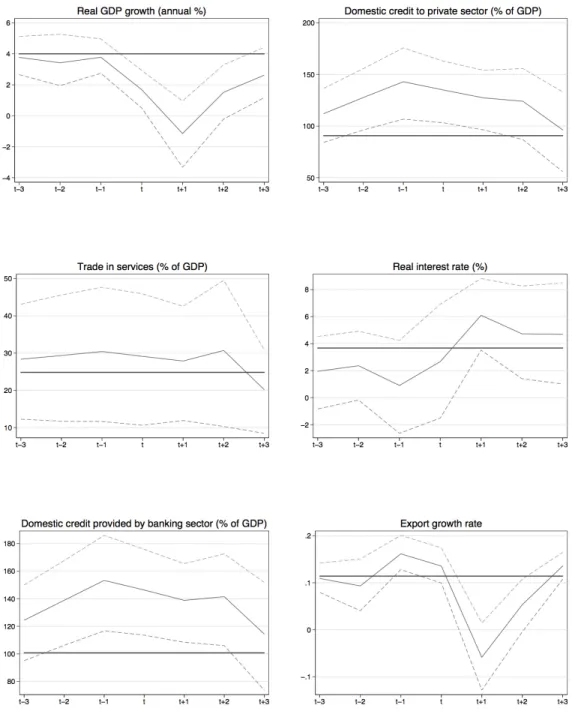
The case of time window ‘t-1, t, t+1’ is given in Figure 5.1 to Figure 5.3 and the case of time window ‘t, t+1, t+2’ is given in Figure 5.4 to Figure 5.7. In the graphs, the bold horizontal line presents the average value of the variable during tranquil periods, and the solid lines stand for the average value of the variable in the interval around the crisis periods, with 3 years before and 3 years after the crisis, among with a 95% confidence interval denoted by the two dotted lines. The time interval for the event study starts from ‘t-3’ and ends at ‘t+3’. The indicator ‘t’ stands for the years in which the crisis indicator variable (which is designed to capture banking, currency and debt crises) is equal to 1 for the first time, which signals the start of a crisis. The event study analysis of the case of ‘t-1, t, t+1’ suggests the following:

• Real GDP growth rate is not only significantly lower during pre-crisis years than the tranquil periods’ average, but it follows the same worsening path during a crisis period as well and it maintains the same downward motion until ‘t+1’. This period involves the shifting from an average of 4 percent to minus 1 percent. Then the recovery period begins.

• Domestic credit to private sector (% of GDP) diverges from the tranquil periods’ average from the beginning of the pre-crisis period; it reaches its peak level just before the crisis and returns to the tranquil average at the end of the analyzed time period ‘t+3’.

• Trade in services (% of GDP) begins with 28 percent, which is above the tranquil periods’ average of 25 percent. Then it deteriorates just before the crisis, at ‘t-1’, and it continues this slow-down until the end of the time interval, where the variable reaches 20 percent.

• Real interest rate starts with 2 units, follows a rapid increase starting from ‘t-1’, this continues during the crisis period, and it reaches to 6 units, which is above the tranquil periods’ average of 3.8. After ‘t+1’ the real interest rate falls down towards the tranquil periods’ average.

• Domestic credit provided by banking sector (% of GDP) starts above the tran-quil periods’ average and it continues increasing. It reaches to its peak level, which is nearly 150, at the time of ‘t-1’ and follows a downtrend and it finishes the time interval below its starting point.

• Export growth rate starts falling down at ‘t-1’. It falls down from 0.15 and reaches to its minimum, which is -0.05, at ‘t+1’. Then it attains its average level near the end of the time interval.

• Total reserve growth starts below its tranquil periods’ average of 0.1. It falls below its tranquil periods’ average at the start of the crisis, ‘t’, and then the recovery procedure begins and it reaches to 0.25 at ‘t+3’.

• FDI to GDP starts with the tranquil periods’ average of 0.2 and it starts falling down by ‘t-1’ and it maintains this throughout the crisis and the recovery starts a while later than the crisis period, ‘t’. But it remains below its starting point at the end of the time interval.

• Deposit rate starts with the tranquil periods’ average and then it starts increas-ing at ‘t-3’. It follows this trend until ‘t+1’ and then its rate of increase gets augmented until ‘t+2’. Then it attains a downward slope towards its tranquil

periods’ average. But at the end of the interval, the deposit rate is still above the tranquil periods’ average.

• Interest rate spread starts with a downward move until ‘t-1’. Then it begins increasing at ‘t-1’ and this continues until ‘t’. It experiences a slight decrease starting with the crisis. Its value remains the same until ‘t+3’, where it is still above the tranquil periods’ average.

• S&P global equity indices (annual % change) starts below the tranquil periods’ average. It increases during the period from ‘t-3’ to ‘t-2’ and then, approaching the crisis, a noticeable decline starts which continues until the crisis hits the economy. Then, it attains an upward trend moving above its tranquil periods’ average. However, the instability continues and the variable reaches the end of the interval with a value, which is way below its tranquil average.

• Bank capital to asset ratio starts with a value of 7.2 percent ratio, which is below its tranquil periods’ average of 7.6. It follows a downward up until ‘t+1’. Then, the recovery begins and the ratio reaches to its tranquil periods’ average back again at the time of ‘t+2’.

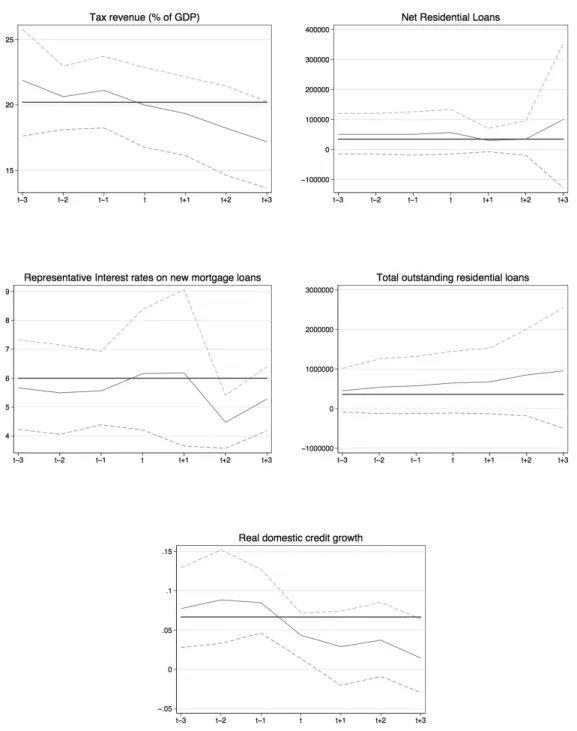
• Tax revenue starts decreasing from a value of 22 percent at ‘t-3’ until ‘t’. Just before the crisis hits the economy at the time of ‘t’, the tax revenue is equal to the its tranquil periods’ average of ∼ 20. Then it maintains it downward trend down to the value of 14 percent.

• The residential loans start above the tranquil periods’ average by approximately 30000 units and then it decreases to the tranquil periods’ average by the crisis period ‘t’. It begins increasing at the end of ‘t+2’.

• Representative interest rate is under the tranquil periods’ average between ‘t-3’ and ‘t-1’. It follows a slightly downward trend during this time interval. After

this falling period it keeps increasing up until ‘t+1’. However, it experiences a sharp decline and reaches to its minimum, at ‘t+2’, 2 years after the crisis hits the economy.

• Total outstanding residential loans follow a sustainable trend with a very slight slope from ‘t-3’ to ‘t+1’, with a value of approximately 500000. After that, it attains a rather higher slope and ends up at around 1000000 where the tranquil periods’ average is around 400000.

• Real domestic credit growth exhibits a sharp decline starting at ‘t-1’ by the value of ∼ 0.09 and it maintains this downward slope until it falls to 0.03 at ‘t+1’. Despite the slight increase seen between ‘t+1’ and ‘t+2’, the value of the variable reaches to its minimum of ∼ 0.02 by ‘t+3’.

All variables, which are chosen as the best performers, varied through tranquil pe-riod to pre-crisis pepe-riod, so the multinomial logistic regression will include all variables mentioned above for ‘t-1, t, t+1’.

The case of ‘t-1, t, t+1’ and the case of ‘t, t+1, t+2’ are different from each other regarding the definitions of the pre-crisis, crisis and tranquil periods. The explanatory variables used in these models and their impacts on predicting crises are different from each other as well.

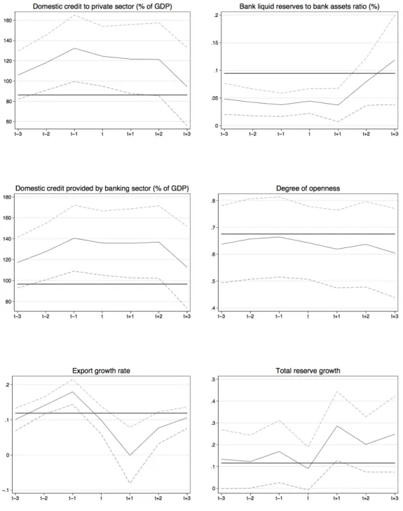
As a result of this, the event study analysis for the case of ‘t, t+1, t+2’ suggests the following:

• Domestic credit to private sector starts above its tranquil periods’ average and even exhibits a rapid increase between ‘t-3’ and ‘t-1’. After this point, a negative movement starts and decline sharpens after ‘t+2’ and the value approaches to its tranquil mean at ‘t+3’.

• Bank liquid reserve to bank asset ratio starts already below its tranquil periods’ value and decreases until ‘t+1’. Then starts a sharp increase, which takes the value even higher than the tranquil mean at the end of the interval.

• Domestic credit provided by banking sector begins on 118, which is above the tranquil period’s average of ∼ 95. Then it maintains an upward trend between ‘t-3’ and ‘t-1’. After that, with a slight decrease starting at ‘t-1’, it maintains a rather flat behavior until it experiences a sharp decrease by ‘t+2’ which takes the value closer to its tranquil mean at ‘t+3’.

• Degree of openness start with 0.65, which is below the tranquil period’s average. It has a downward trend in the period between ‘t-1’ and ‘t+1’. Then it enters into a recovery period, however at ‘t+3’, it is still below its staring value of 0.65, which is also below its tranquil periods’ average.

• Export growth rate begins below the tranquil periods’ average, and then it has a sharp fall between ‘t-1’ and ‘t+1’, in which it falls way below the tranquil average of 0.12 down to 0. Then it enters the recovery period, and finishes at 0.9 but it cannot reach to the tranquil periods’ average.

• Total reserve growth begins with ∼ 0.14 which is slightly above the tranquil periods’ average of 0.12. Then, it starts decreasing at ‘t-1’, just the year before the crisis. It maintains this downward trend until the crisis, ‘t’ and then it enters into a recovery and attains the value of 0.25 at ‘t+3’, three years after the crisis.

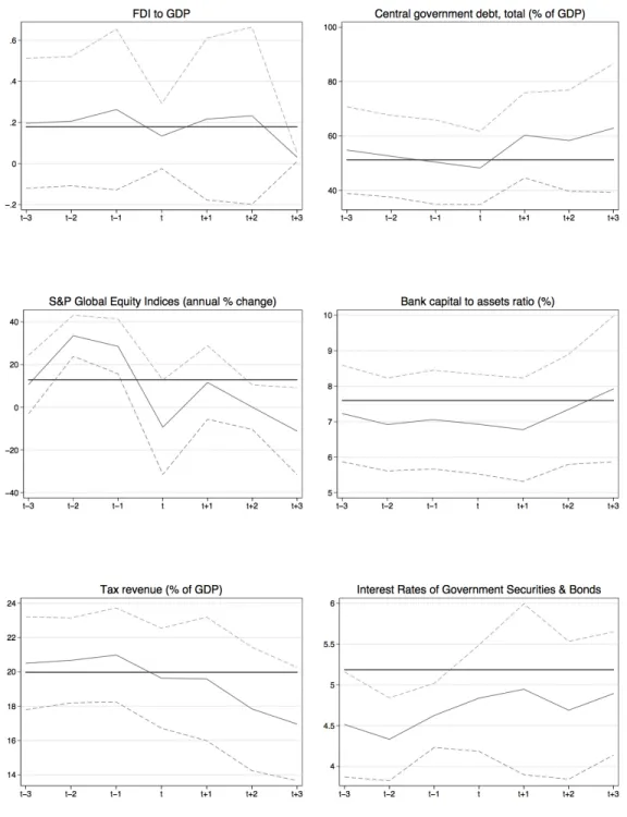
• FDI to GDP starts at a point at which it is slightly above the tranquil periods’ average. Then it starts decreasing by the year just before the crisis and reaches to its minimum at ‘t’, the start of the crisis. Then it keeps increasing during the period from ‘t’ to ‘t+2’. However, the instability continues and it almost becomes 0 at ‘t+3’, which is below its tranquil mean.

• Central government debt begins above the tranquil periods’ average. When the crisis hits the economy at ‘t’, it starts increasing from 50 percent to 60 percent within the year following the crisis. By ‘t+3’, it is still above the tranquil periods’ average.

• S&P global equity indices falls from nearly 30 percent to minus 10 percent in the pre-crisis period. Then the recovery starts and in this period, it increases to 10 percent, which is a little bit below its tranquil periods’ average. Then, it experiences a sharp fall again.

• Bank capital to asset ratio decreases in the period between ‘t-1’ and ‘t+1’. Then it gets into the recovery period and returns to and exceeds its average level of 7.6 between ‘t+2’ and ‘t+3’.

• Tax revenue starts at about 21, which is above the tranquil periods’ average of 20. Then it enters into a downfall by ‘t-1’, the year just before the crisis. It falls by an amount of nearly 5 percent until ‘t+3’. It finishes at 14 percent, which is far below the tranquil periods’ average.

• Interest rate of government securities and government bonds is generally below the tranquil periods’ average, although it approaches to the average between ‘t-2’ and ‘t+1’. Then it enters into a falling period and starts increasing again 2 years after the crisis, but it is still below its average value at ‘t+3’.

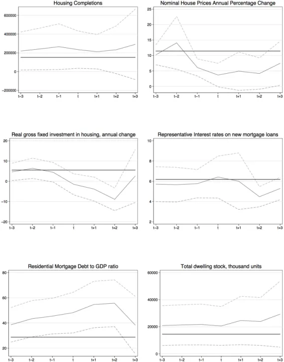
• Housing completions decrease by 50000 units in the period between ‘t-1’ and ‘t+1’. After this period, it attains an upward trend.

• Nominal house prices annual percentage change reacts to the upcoming crisis with a very sharp fall from nearly 14 percent to 4 percent until the crisis hits the economy. After the crash, it enters into the recovery period but after the crisis, it is seen that the impact is still effective on the nominal house prices annual percentage change because it still cannot reach to its tranquil periods’ average at ‘t+3’.

• Real gross fixed investment in housing responds to the crisis earlier than its crash. It decreases from 7 percent to minus 9 percent during the period between ‘t-2’ and ‘t+2’. The downward trend continues during the adjustment period and a strong recovery is observed starting from ‘t+2’, two years after the crisis. • Representative interest rates on new mortgage loans increases in the pre-crisis period up until the crisis hits the economy. Then, by the beginning of the recov-ery period if falls below the tranquil periods’ average by reaching the minimum at ‘t+2’ and returns from that point to try attaining the tranquil mean again. • Residential mortgage debt to GDP ratio diverges from the tranquil period’s

average. The residential mortgage debt to GDP ratio starts from nearly 38 percent at ‘t-3’ and at the end of ‘t+2’ it becomes 58 percent. After ‘t+2’, a recovery is observed and the value starts decreasing to approach to the tranquil mean, however, at ‘t+3’, it is still nearly at 39 percent, which is higher than

the tranquil average of 25 percent. This signifies that impact of crisis is still effective on the variable even 3 years after the crisis.

• Total dwelling stock decreases by nearly 2000 units between the pre-crisis and the crisis period. After the recovery period, there occurs a huge rise in the amount of dwelling stock, approximately by 10000 units until the end of the recovery period.

• Import growth rate is also affected from the crisis. Its tranquil periods’ average is equal to 0.12. There is a sharp decline during the period between ‘t-1’ and ‘t+1’ from a value of 0.19 to 0. Only then, the recovery begins, and the value reaches to its tranquil mean again at ‘t+3’.

• International reserve growth follows a stable but very slight downward trend, which is always lower than the tranquil periods’ average. After the crisis bursts, it starts following an upward trend till the end of the period it slightly exceeds the pre-crisis period’s value.

• Current account to GDP variable’s tranquil periods’ average is -0.01 and it is worsening from the very beginning of the pre-crisis period. It falls down to -0.03 at ‘t-1’. After a recovery period with some fluctuations, it manages to reach to its average value at ‘t+3’ again.

• Real domestic credit growth’s tranquil periods’ average is 0.06. The downward motion starts at ‘t-2’, however, it is much more significant in the period between ‘t-1’ to ‘t+1’ where the value decreases from ∼ 0.09 to 0 moving below the tranquil average. For the rest of the recovery period, the fluctuations continue for making it possible to attain the average value again.

• Change in terms of trade is generally close to its tranquil mean in the pre-crisis period. However, in the recovery times, there occur some significant fluctuations in the variable due to the effects of the crisis.

• Rate of change of housing price to GDP growth ratio responds the crisis by falling down in the period between ‘t-3’ and ‘t+1’, with a decrease from 11 percent to -4 percent. Then in the adjustment period between ‘t+2’ and ‘t+3’, it reaches to its tranquil mean, which is about 2.

All variables, which are chosen as the best performers, varied through tranquil pe-riod to pre-crisis pepe-riod, so the multinomial logistic regression will include all variables mentioned above for ‘t, t+1, t+2’.

5.2

Empirical Analysis

In choosing which variables are more appropriate to be used for crisis prediction, the multinomial logistic regression, which was firstly applied by Bussiere and Fratzscher (2002) to constitute a new approach to predict crisis, was used as an estimation tool [Bussiere and Fratzscher(2002)]. In applying this approach, the time interval is divided into three sub-periods as a tranquil period, a pre-crisis period and an adjustment period. In the tranquil period, the economy does not have a risk of crisis and the economic variables follow a predictable path. In the pre-crisis period, the economic variables start giving some signals about the coming crisis by deviating from their average path. In the adjustment period, the economy has already been hit by the crisis and measures are being taken for the recovery. Because of this, the economic variables start approaching to their tranquil regime values again and they follow a more predictable path.

This analysis differs from the literature by the fact that it focuses on the impact of the housing market on the crisis prediction. It uses two different techniques - in terms of the time windows they use for prediction - and investigates the prediction powers of these different techniques. It aims predicting not only one but all three types of crises as banking, currency and debt.

In the multinomial logistic regression, the probabilities for a country being in each of the mentioned three different periods is calculated as the following:

P r(Yi,t = 0) = 1 1 + eXi,tβ1 _{+ e}Xi,tβ2 P r(Yi,t = 1) = eXi,tβ1 1 + eXi,tβ1 _{+ e}Xi,tβ2 P r(Yi,t = 2) = eXi,tβ2 1 + eXi,tβ1 _{+ e}Xi,tβ2 (5.1)

When Y is equal to 0, it implies that, the economy is in the tranquil period. If Y is equal to 1, it means that the economy is in the pre-crisis and in the case of Y being equal to 2, the economy is in the adjustment regime.

Here, β1 and β2 indicate the marginal impact of a change in the explanatory

variables on the probability of being in pre-crisis or adjustment period relative to the probability of being in the tranquil period respectively as shown below:

P r(Yi,t = 1) P r(Yi,t = 0) = eXi,tβ1 P r(Yi,t = 2) P r(Yi,t = 0) = eXi,tβ2 (5.2)

The multinomial logistic regression consists of three steps and while constructing these steps the methodology of Ciarlone et al was followed [Ciarlone and Trebeschi(2005), Ciarlone and Trebeschi(2006)]:

- First of all, the multinomial logistic regression was run for each of the 111 vari-ables independently from each other. Although it is a fact that the multinomial logistic regression is meaningful if both the relation between the variables and their deviations are taken into consideration, the aim of this procedure was controlling the Wald statistics and the sign of the coefficient of each variable before beginning the group analysis. This step is helpful for determining the significance and the impact of the variables on the estimation. Indeed, there occurred some problematic cases in choosing the variables for constructing the model. There were some variables (such as fiscal surplus to GDP ratio), which were statistically significant and their predictive powers were very high. How-ever, it has been realized in the final step that those variables would destroy the validity of the constructed model by enlarging its confidence interval and destroying the Wald statistics. As a result, this makes it impossible to construct