DOI: 10.1002/nla.2158
R E S E A R C H A R T I C L E
On compact vector formats in the solution of the chemical
master equation with backward differentiation
Tuˇgrul Dayar
1M. Can Orhan
21Department of Computer Engineering,
Bilkent University, Ankara, Turkey
2Kanava Technologies, Ankara, Turkey
Correspondence
Tuˇgrul Dayar, Department of Computer Engineering, Bilkent University, TR–06800 Bilkent, Ankara, Turkey. Email: [email protected]
Funding information
Alexander von Humboldt Foundation; Scientific and Technological Research Council of Turkey, Grant/Award Number: 2211-A
Summary
A stochastic chemical system with multiple types of molecules interacting through reaction channels can be modeled as a continuous-time Markov chain with a countably infinite multidimensional state space. Starting from an ini-tial probability distribution, the time evolution of the probability distribution associated with this continuous-time Markov chain is described by a system of ordinary differential equations, known as the chemical master equation (CME). This paper shows how one can solve the CME using backward differentiation. In doing this, a novel approach to truncate the state space at each time step using a prediction vector is proposed. The infinitesimal generator matrix associ-ated with the truncassoci-ated state space is represented compactly, and exactly, using a sum of Kronecker products of matrices associated with molecules. This exact representation is already compact and does not require a low-rank approxima-tion in the hierarchical Tucker decomposiapproxima-tion (HTD) format. During transient analysis, compact solution vectors in HTD format are employed with the exact, compact, and truncated generated matrices in Kronecker form, and the linear systems are solved with the Jacobi method using fixed or adaptive rank control strategies on the compact vectors. Results of simulation on benchmark mod-els are compared with those of the proposed solver and another version, which works with compact vectors and highly accurate low-rank approximations of the truncated generator matrices in quantized tensor train format and solves the linear systems with the density matrix renormalization group method. Results indicate that there is a reason to solve the CME numerically, and adaptive rank control strategies on compact vectors in HTD format improve time and memory requirements significantly.
K E Y WO R D S
backward differentiation, chemical master equation, compact vector, continuous-time Markov chain, Kronecker product
1
I N T RO D U CT I O N
A stochastic chemical system with multiple types of molecules interacting through reaction channels can be modeled as a continuous-time Markov chain (CTMC) with a countably infinite multidimensional state space. In this context, a state is a row vector with elements representing the number of molecules of each type present in the system. A state
Numer Linear Algebra Appl. 2018;25:e2158. wileyonlinelibrary.com/journal/nla Copyright © 2018 John Wiley & Sons, Ltd. 1 of 21 https://doi.org/10.1002/nla.2158
transition corresponds to a reaction channel that is expressed by a state change vector and a state-dependent transition rate function. Starting from an initial probability distribution, time evolution of the probability distribution associated with the multidimensional CTMC is described as a system of linear first-order ordinary differential equations (ODEs), known as the chemical master equation (CME; or forward Kolmogorov equation). The goal is to compute the transient probability distribution of the stochastic chemical system at a particular time by solving the CME whose coefficient matrix is the infinitesimal generator of its underlying CTMC. A detailed overview on transient analysis of stochastic chemical systems may be obtained, for instance, from the extensive review by Goutsias et al.1
Analytical solution of the CME is possible only in a few simple cases2–5; therefore, other approaches are considered.
A popular approach is to use the stochastic simulation algorithm (SSA)6,7in which sample trajectories are generated by
simulating reaction events. SSA is said to be exact in the sense that every reaction event is simulated. Approximation tech-niques that avoid simulating every reaction event such as tau-leaping methods8,9and system-partitioning methods10–12
are suggested to reduce computational complexity by trading off accuracy. A drawback of simulation techniques is that they require a large number of trajectories to obtain sufficiently accurate estimates and they are inefficient especially for estimating probability distributions.
Another approach is to solve the CME numerically. This is a formidable task because the size of the CME increases exponentially with the number of dimensions even when an upper bound is applied to the number of molecules in the system. Munsky et al.13proposed the finite state projection (FSP) algorithm to approximate the actual probability
distri-bution. The FSP algorithm gradually expands the truncated state space by adding states that are reachable within a certain number of transitions and solves the truncated CME until the accuracy of the approximate solution meets a prespecified tolerance. The algorithm uses a number of molecule types, that is, the number of dimensions, in limiting reachability during the truncated state space expansion process. Unfortunately, this strategy yields a truncated state space includ-ing many states with negligible probability. Furthermore, the matrix scalinclud-ing and powerinclud-ing method (see pp. 416–417 in the work of Stewart14) employed to solve the truncated CME becomes inefficient as the size of the system increases.
Hence, several variants of the FSP algorithm such as multiple time interval FSP,15 Krylov-FSP,16,17 optimal FSP,18 and sliding window19methods are proposed to solve the CME more efficiently. These methods differ from each other by the
choice of the truncated state space and the technique employed to solve the truncated CME. We refer to the survey by Dinh et al.20for an overview of the FSP algorithm and its variants.
Accurate approximation of the probability distribution requires the truncated state space to be large in many cases. Some numerical methods take a hybrid approach and combine the CME solver with other techniques to improve execution time and memory requirement by trading off accuracy.21,22Other numerical methods reduce the degrees of freedom, that is,
the number of unknowns, in the CME by sparse grids,23,24discrete orthogonal polynomials,25,26and sparse wavelets.27,28
In essence, these methods represent the probability distribution as a linear combination of basis functions. Although the degrees of freedom become smaller, these methods still suffer from the curse of dimensionality, that is, memory requirements and computational cost scaling exponentially with the number of dimensions.
In order to overcome the curse of dimensionality, low-rank approximation techniques that represent multidimensional arrays (or tensors) compactly are employed in many application areas (see, for instance, the work of Grasedyck et al.29).
Canonical polyadic (CP) decomposition30,31is a compact representation of a tensor, where the multidimensional array is
given as a sum of Kronecker products of smaller vectors or rank-one tensors. Jahnke et al.32 projected the dynamics of
the system onto a manifold of all tensors in CP decomposition format with a predetermined maximal tensor rank. The rank bound is chosen based on the initial distribution and kept constant. However, they advise an adaptive rank control strategy because it is not possible to estimate the rank of a vector in CP decomposition format that approximates the solution of the CME with a desired accuracy. Hegland et al.33employed the implicit Euler method to solve the CME and store probability vectors in CP decomposition format. Therein, a bound on the ranks is not chosen, and they suggested to reduce ranks after algebraic tensor operations using various procedures.34 However, this approach appears to pose
problems in practice because there is no robust and efficient algorithm to approximate the CP decomposition with low ranks using any desirable accuracy for tensors having more than two dimensions.
The Tucker decomposition35represents a d-dimensional tensor as the multiplication of a d-dimensional core tensor
and a basis matrix along each dimension. The higher-order singular value decomposition (HOSVD)36provides a simple
and nearly optimal solution to approximate a tensor in the Tucker decomposition format with a user-controlled error. However, the memory requirement of the core tensor scales exponentially with the number of dimensions. The tensor train (TT) decomposition37is a low-rank approximation technique that avoids this exponential dependence on the number
of dimensions, d. The TT decomposition is extended to the quantized TT (QTT) decomposition,38 which is shown to
molecule, a quantization size of 2 is used, and m is a power of 2; QTT provides the way for the best possible compression rate for data within the chosen and rank-structured dimensional splitting model in the auxiliary dimension D = dlog2m.
We refer to the paper by Khoromskij39 for an overview of related tensor numerical methods. A Kronecker-based solver
for a multiparticle probabilistic model in the TT and QTT formats has first been applied to the Fokker–Planck equation,40
which is closely related to the CME.
The truncated generator matrix associated with the CME has been shown to have low TT and QTT ranks,41,42 and it
is possible to represent the solution of the truncated CME compactly in QTT format and reduce memory requirements of solution vectors.42,43 It seems that a compact vector in QTT format can be multiplied by a matrix only in the same
format, and the linear system at each step can be solved using an iterative method such as the density matrix renormal-ization group (DMRG) method.44DMRG is an optimization-based method that is also used in solving linear systems and
has been used before to solve the CME with the QTT format.43At each DMRG iteration (or sweep), core matrices
corre-sponding to consecutive virtual dimensions are aggregated; each aggregated system is solved directly or using an iterative method such as generalized minimal residual, and the result of the aggregated system is disaggregated. The peak effi-ciency of the QTT approach is achieved if quantization in the time variable is also implemented,42the so-called time–space
approximation scheme.
Another low-rank approximation technique that admits user-controlled error is the hierarchical Tucker decomposi-tion (HTD).45–48HTD may be considered as a generalization of the TT decomposition in which basis and core matrices
are related through a tree structure with logarithmic depth in the number of dimensions that reduces the complexity of the Tucker decomposition by hierarchically splitting the core tensor into core matrices. An advantage of the HTD representation for our purposes is that the multiplication of a compact solution vector in HTD format with a sum of Kro-necker products is a well-defined operation49and has recently been used in the steady-state analysis of Kronecker-based
CTMCs.50In the CME setting, such a Kronecker-based Markovian analysis with vectors in HTD format is possible under
the separability assumption of transition rates.7,25,32,43,51,52To the best of our knowledge, the HTD format has not been
employed in the transient analysis of the CME so far.
Backward differentiation formulae (BDF; see pp. 446–448 in the work of Stewart14) are a class of implicit multistep
methods to solve ODEs. The k-step BDF method, denoted BDFk, keeps the approximations of solutions at k previous time steps and computes the solution at the current time step by solving a linear system. BDFk methods have local truncation error proportional to the kth power of the step size and, therefore, are said to be of order k. They have two major advan-tages in solving the CME. First, BDFk provides an efficient solver for stiff systems in which the solution contains rapidly decaying transient terms. Stiffness generally manifests itself when reaction rates occur at different time scales, and this is the case for many realistic systems. Second, a prediction of the solution can be given as a linear combination of previous solutions (see p. 150 in the work of Ascher et al.53), and local truncation error can be obtained from the difference between
prediction and solution at that step.54The prediction vector provides a good estimate of the solution, and contrary to the
FSP algorithm, it is possible to choose a truncated state space that includes most of the probability mass without having to compute the solution of the truncated CME at that step.
In this paper, we propose a BDFk solver for the CME, which uses a prediction vector to truncate the countably infinite state space at each time step. Then, the truncated generator matrix associated with the CME at each time step is repre-sented compactly, and exactly, using a sum of Kronecker products of matrices associated with molecules.55 This exact
representation, which has been used in the Kronecker-based modeling and analysis of finite multidimensional CTMCs56
for many years, is already compact and does not require a low-rank approximation for compactness in the HTD format. Following recent results from the steady-state analyses of Kronecker-based CTMCs with compact vectors,50 however,
solution vectors in the HTD format are employed in the proposed BDFk solver with the exact, compact, and truncated generator matrix in Kronecker form during transient analysis. The linear system at each time step of BDFk is solved iter-atively by the Jacobi method, which splits the coefficient matrix into diagonal and negated off-diagonal matrices at the outset so that the iteration vector is multiplied by the negated off-diagonal matrix and inverse of the diagonal matrix at each iteration. Computation of the inverse of the diagonal matrix at the outset is convenient. To that end, the diagonal of the coefficient matrix is obtained in HTD format, and the elementwise reciprocal of this compact vector is computed iteratively using the Newton–Schulz method.47 If an iteration vector is not close to the solution, an accurate
computa-tion of the vector should not be necessary. Furthermore, the imposed accuracy may yield addicomputa-tional time and memory requirements. Therefore, we propose adaptive rank control strategies in Newton–Schulz and Jacobi iterations that allow relatively inaccurate computation of iteration vectors.
In summary, at each time step of the proposed BDFk solver, truncation takes place on the state space due to its countable infiniteness, in the solver due its use of a finite number of backward differences, and in the low-rank approximation of solution vectors to control the error in the approximation. The proposed approach that uses compact vectors in HTD
format does not need to compute a low-rank approximation to the truncated generator matrix at each time step of the transient solver. This is expected to yield memory and time savings. Furthermore, the Jacobi iterative method used in solving the linear system requires only a small number of supplementary vectors compared with more sophisticated iterative solvers, and this is expected to result in further savings, especially when only a few iterations of the method end up being executed at each time step.
Although we follow in our research the basic algorithms from the htucker47,48and tt-toolbox57Matlab toolboxes,
the code is implemented in C58within the NSolve package of the Abstract Petri Net Notation toolbox,59,60which is used
in the analysis of Kronecker-based CTMCs, and calls some LAPACK functions.61Results of simulation62on benchmark
models are compared with those of the proposed solver and another version, which works with compact vectors and highly accurate low-rank approximations of the truncated generator in QTT format and solves the linear system at each time step with the DMRG method. Results indicate that there is a reason to solve the CME numerically, and adaptive rank control strategies on compact solution vectors in HTD format improve time and memory requirements significantly when fixed rank control strategies lead to inefficient ODE solvers.
Throughout the paper, calligraphic uppercase letters are used for sets. Vectors and matrices are represented respectively with boldface lowercase and boldface uppercase letters. All vectors are row vectors except e and eh, which represent a
column vector of ones and the hth column of the identity matrix, respectively. 1 denotes a row vector of ones, and I denotes the identity matrix. Lengths of vectors and sizes of identity matrices are determined from the contexts in which they are used. A(, ) is the submatrix of A where rows and columns are selected respectively from the sets and , and A(x, y) is the value of matrix A corresponding to element (x, y). Consistently, a(x) is the value of vector a at state x, and a() is the subvector of a including the values of a(x) for x ∈. diag(a) denotes a matrix with the entries of vector a along its diagonal and 0 elsewhere. The sets of integers, positive integers, and nonnegative integers are denoted byZ,Z>0,Z≥0, and the sets of reals, positive reals, and nonnegative reals are denoted byR,R>0,R≥0, respectively. Finally,T, ×,⊗, and ⋆
denote respectively the transposition, Cartesian product, Kronecker product, and elementwise multiplication operators. The next section provides background on CME, BDF, and HTD. The third section describes implementation details of the proposed CME solver. The fourth section discusses results of numerical experiments, and the fifth section concludes the paper.
2
BAC KG RO U N D
2.1
Chemical master equation
We consider a CTMC describing the dynamics of a stochastic chemical system with d types of molecules interacting through J reaction channels. Let {S(t) = (S1(t), … , Sd(t)) ∈ , t ≥ 0} be the stochastic process associated with the d-dimensional CTMC, whereh ⊆ Z≥0 is the set of states that molecules of type h can be in, and = ×dh=1his the
product state space of the system, which is potentially infinite. The underlying CTMC can be described by J transition classes each corresponding to a reaction channel as in the next definition.55
Definition 1. A pair (𝛼(j), v(j))is said to be transition class𝑗 ∈ {1, … , J}, where 𝛼(𝑗)∶ →R
>0and v(𝑗) ∈Z1×dare respectively the transition rate function and the state change vector.
We assume the separability of transition rate function𝛼. That is, there exist 𝛾(𝑗)∈R>0and𝛼(𝑗)
h ∶h→R≥0such that 𝛼(𝑗)(s) =𝛾(𝑗) d ∏ h=1 𝛼(𝑗) h (sh)
for s = (s1, … , sd) ∈ and j = 1, … , J. This separability assumption holds for elementary reactions that are also building
blocks in more complicated reaction kinetics.7,25,32,43,51,52
It is possible to represent the infinitesimal generator matrix underlying the multidimensional CTMC as a sum of Kro-necker products of matrices associated with molecules. The following relates molecules and transition classes by defining transition matrices.55
Definition 2. The transition rate matrix of molecule h ∈ {1, … , d} for transition class 𝑗 ∈ {1, … , J}, denoted by S(h𝑗)∈R|h|×|h| ≥0 , is given elementwise as S(h𝑗)(sh, s′h) = { 𝛼(𝑗) h (sh) if s ′ h=sh+v (𝑗) h 0 otherwise for sh, s ′ h∈h.
The infinitesimal generator matrix includes a diagonal corrector that ensures that row sums are zero; therefore, it is convenient to let D(h𝑗)=diag(S(h𝑗)e) ∈R|h|×|h|
≥0 for h = 1, … , d and j = 1, … , J. Then, the infinitesimal generator matrix
can be written as Q = J ∑ 𝑗=1 S(𝑗)− J ∑ 𝑗=1 D(𝑗) with S(𝑗)=𝛾(𝑗) d ⨂ h=1 S(h𝑗) and D(𝑗)=𝛾(𝑗) d ⨂ h=1 D(h𝑗) for𝑗 = 1, … , J. Finally, the CME that describes the time evolution of the stochastic chemical system is given by
𝜕pt
𝜕t =ptQ with initial condition pt||t=0=p0,
where pt ∈R1×≥0||is the probability distribution (row) vector of the system at time t≥ 0, satisfying pte = 1.
Having defined the initial value problem to be solved, let us now turn to its solution through BDF.
2.2
Backward differentiation formulae
BDF are a class of implicit multistep methods that are widely used to cope with stiffness in the solution of ODEs. In this class of solvers, time is discretized and solutions at intermediate time steps are approximated using backward differences (see p. 125 in the work of Ascher et al.53). It is not possible to use a BDF solver when the ODE system has a countably
infinite number of equations and unknowns; however, the ODE system may be truncated by assuming that the probability of the system being at a state outside the finite truncated state space is zero.
Let us denote bynthe truncated state space at time step n such thatn⊂ and nis finite. In order to avoid using
two levels of subscripts with ptwhen describing the BDF method, we omit t and the step size, Δt, in the notation, and let the vector pn−i ∈ R1×|≥0 n−i| hold the probabilities of the system being at states inn−iat time (tn−iΔt)for i = 0, … , k.
Then, for a constant step size Δt> 0, the BDF method of order k, denoted BDFk, at time step n is given by
k ∑ i=1 1 i∇ ip n= ΔtpnQn with Qn=Q(n, n),
where the backward difference vectors ∇ip
n∈R1×|n|are recursively defined as
∇0pn=pn for n ∈Z≥0 and ∇ipn= ∇i−1pn− ∇i−1pn−1 for i =1, … , k and n ∈Z>0.
Here, pn∈R1×≥0|n|is the solution to be obtained at time step n.
Note that BDFk may be rewritten as a linear system in the form
pn(I −𝜃kΔtQn) = k−1
∑
i=0
𝛽k,i∇ipn−1, (1)
where𝜃kand𝛽k,0, … , 𝛽k,k−1are real numbers defined by BDF order k. For instance,𝜃5=60∕137,𝛽5,0=1,𝛽5,1=77∕137, 𝛽5,2=47∕137,𝛽5,3=27∕137, and𝛽5,4=12∕137 when k = 5.
The leading term of the BDFk local truncation error can be approximated as
rn≈ 1 k +1 ( pn−p(0)n ) , (2) where p(0)n = k ∑ i=0 ∇ipn−1
is the prediction vector.54
The probability of the system being in a state changes over time. Hence, at each time step, the truncated state spacen
needs to be chosen such that the probability of the system being outsidenis small. One possible approach is solving (1)
and expanding the truncated state space until it includes most of the probability mass as in the FSP algorithm.13However,
it is possible to take a different and more efficient approach. The prediction vector p(0)n ∈R1×|n|
≥0 is a good estimate of the
solution at time tn=tn−1+ Δt. Hence, the truncated state spacenwill capture most of the probability mass at time tnif
∑
s∉np
(0)
n (s) is small. This approach allows us to choose the truncated state space before solving (1) because the backward
difference vectors ∇0p
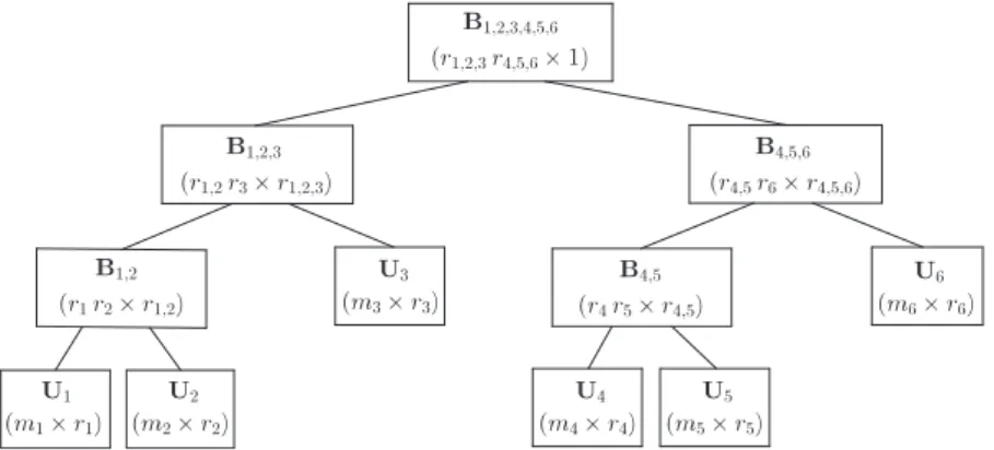
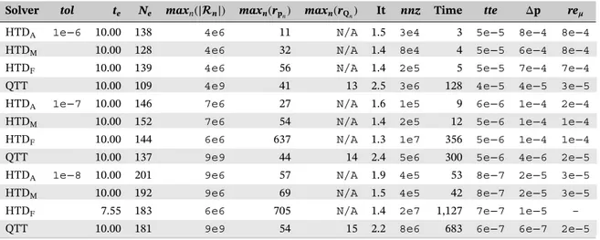
FIGURE 1 Matrices forming x in hierarchical Tucker decomposition format for d = 6
Backward differences are also very suitable for adjusting the step size.54 Letting P and P∗ denote respectively the
matrices with backward differences for old step size Δt and new step size Δt∗≠ Δt as in
P =[(∇1pn−1 )T , … ,(∇kpn−1 )T] and P∗=[(∇∗1pn−1 )T , … ,(∇∗kpn−1 )T] ,
the new backward difference vectors may be obtained from P∗ = P ̄R∗̄U∗, where ̄R∗ and ̄U∗ are (k × k) matrices given
elementwise as ̄R∗(i, i′) = 1 i! i−1 ∏ l=0 ( l − i′(Δt∗∕Δt)) and ̄U∗(i, i′) = 1 i! i−1 ∏ l=0 (l − i′) for i, i′=1, … , k.
The next section provides a short description of HTD and operations that are used in the implementation of BDFk.
2.3
Hierarchical Tucker decomposition
A column vector x of length∏dh=1mhin Tucker decomposition format35can be expressed as
x = (U1⊗ · · · ⊗ Ud)c,
where Uhis an (mh×rh)orthogonal basis matrix for dimension h with h = 1, … , d, and c is a vector of length
∏d h=1rh.
Memory requirement for this representation scales exponentially with d.
HTD45–48employs a hierarchical splitting of dimensions 1, … , d to represent vector c using smaller matrices.
Definition 3. Let be a binary tree with each node represented by a subset of {1, … , d}. Then, is said to be a
dimension tree if the root node is {1, … , d}, each parent node is a disjoint union of its children, and there are d leaf nodes with each leaf node represented by a different singleton from {1, … , d}.
Given orthogonal matrices Ūt, Ūtl, and Ūtr, there exists a (r̄tlr̄tr×r̄t) transfer matrix B̄tsuch that
Ūt = (Ūtl⊗ Ūtr)B̄t, (3)
where ̄tland ̄trare the left and right children of nonleaf node ̄t (see lemma 2.1 in the work of Kressner et al.48), respectively.
Then, by recursively substituting in (3), vector x = U1, … ,dcan be represented by d orthogonal basis matrices U1, … , Ud
and (d − 1) transfer matrices B̄tfor ̄t ∈ ( ), where ( ) is the set of nonleaf nodes of binary tree . A possible decomposition for vector x with d = 6 can be written as
x = (U1⊗ U2⊗ U3⊗ U4⊗ U5⊗ U6)c with c = (B1,2⊗ Ir3⊗ B4,5⊗ Ir6) (B1,2,3⊗ B4,5,6)B1,2,3,4,5,6 for the corresponding dimension tree in Figure 1.
Memory requirement for matrices in the dimension tree associated with the HTD format is bounded by the following48:
(dmmaxrmax+ (d −2)r3max+rmax2 ) with rmax=max
̄t (r̄t) and mmax=max(m1, … , md).
A matricization of dimensions corresponding to ̄t may be obtained by taking ̄t as the row index and̄s = {1, … , d}∖{̄t} as the column index of the d-dimensional vector x. The orthogonal matrix Ūt has in its columns the singular vectors associated with the largest r̄tsingular values (see pp. 76–79 in the work of Golub et al.63) of the matricization of dimensions
corresponding to ̄t. Hence, we have the concepts of “hierarchy of matricizations” and “HOSVD”, and r̄tis the rank of the truncated HOSVD.36,47,64
Now, we provide short explanations for operations that are used in the implementation of BDFk in HTD format.
2.3.1
Representing a Kronecker product of vectors in HTD format
Let x = ⊗d
h=1xhbe a vector, where xhis a vector of length mh. Then, x may be represented in HTD format with basis
matrices Uh=xhfor h = 1, … , d and transfer matrices B̄t=1.
2.3.2
Aggregation of dimensions of a vector in HTD format
Let x be a vector in HTD format with basis matrices Uh′for h′=1, … , d and transfer matrices B̄tforming c. Then, the vector obtained by aggregating all dimensions except dimension h of vector x can be written as
g(x) h = (h−1 ⨂ h′=1 1mh′⊗ Imh⊗ d ⨂ h′=h+1 1mh′ ) x = (h−1 ⨂ h′=1 1mh′Uh′⊗ Uh⊗ d ⨂ h′=h+1 1mh′Uh′ ) c.
The vector g(hx)∈R|h|×1is in HTD format with basis matrices
̃Uh′= {
Uh if h′=h
1mh′Uh′ otherwise
and transfer matrices B̄tforming c. The flat representation of g(hx)may be obtained by computing the basis matrices at the leaves and by moving toward the root in O(rmax(dmmax+r2max+mmaxrmax))floating-point operations (flops).
2.3.3
Multiplication of a vector in HTD format with a sum of Kronecker products
Let A = ∑J𝑗=1⊗d h=1A
(𝑗)
h and x be a vector in HTD format with orthogonal basis matrices Uhand transfer matrices B̄t
forming c. Then, the vector y = Ax may be written as
y = J ∑ 𝑗=1 y(𝑗) with y(𝑗)= ( d ⨂ h=1 A(𝑗) h Uh ) c.
Hence, the vector y( j)is in HTD format with basis matrices A(𝑗)
h Uhand transfer matrices B̄tforming c.
2.3.4
Addition of vectors in HTD format
The addition of vectors in HTD format is studied before.47Therein, three algorithms are presented, and the best approach
seems to be adding and truncating each vector one by one (see algorithm 7 on p. 23 in the work of Kressner et al.47). The
significance of algorithm 7 is that it is possible to impose an accuracy of tol on the truncated vector by choosing the rank
r̄tin node ̄t based on dropping the smallest singular values whose squared sum is less than or equal to tol2∕(2d − 3) (see pp. 18–19 in the work of Kressner et al.47) when adding two vectors. The number of flops for adding J vectors with this
algorithm becomes O(d J2r2
max(mmax+rmax2 +Jrmax)).
2.3.5
Computing the 2-norm of a vector in HTD format
The computation of the maximum value in magnitude of the elements of a vector in HTD format seems to be costly. Therefore, instead of the maximum (i.e., infinity) norm of vector x in HTD format, we consider the computation of the 2-norm of vector x given by||x||2 =
√
xTx. The scalar||x||
2can be obtained by computing the inner products of two
compact vectors in HTD format (see algorithm 2 on p. 14 in the work of Kressner et al.47). The number of flops for this
algorithm is O(r2
max(drmax2 +mmax)).
2.3.6
Computing the elementwise multiplication of two vectors in HTD format
The elementwise multiplication of two matrices X and Y with given SVDs (see pp. 76–79 in the work of Golub et al.63)
X = UXΣXVTX and Y = UYΣYVYT results in X⋆ Y ∶= ( UX⊙TUY ) (ΣX⊗ ΣY) ( VX⊙TVY )T ,
where⊙Tdenotes a transposed variant of the Khatri–Rao product.34More specifically, the ith row of the (m × r
ArB)matrix
A⊙TB is the Kronecker product of the the ith rows of the (m × r
A)matrix A and the (m × rB)matrix B. This implies that
the elementwise multiplication X⋆ Y has rank equal to the multiplication of the ranks of the matrices X and Y.
The situation for elementwise multiplication of two vectors x and y in HTD format is no different if SVD is replaced with HOSVD (see pp. 24–25 in the work of Kressner et al.47). As for the multiplication of two vectors in HTD format, the
vector x⋆ y may be truncated directly while computing the basis and transfer matrices. During truncation, it is possible to impose an accuracy of tol on the truncated HOSVD by choosing the rank r̄tin node ̄t based on dropping the smallest singular values whose squared sum is less than or equal to tol2∕(2d − 3), as it is done in the addition of two vectors.
2.3.7
Computing the elementwise reciprocal of a vector in HTD format
In the Jacobi method, the iteration vector needs to be multiplied by the reciprocal of diagonal elements of the coefficient matrix. Because it is costly to generate each element of a vector in HTD format, an iterative method such as Newton–Schulz method (see p. 28 in the work of Kressner et al.47) can be employed to compute the elementwise reciprocal of a vector
in HTD format as in Algorithm 1. In this method, the elementwise reciprocal vector xinv is initialized to a vector with each element having the reciprocal of the 2-norm of the input vector x. The algorithm stops if the relative 2-norm of (e − x⋆ xinv(it−1))is smaller than the tolerance rcp_tol as in elem_reciprocal.m of htucker_toolbox47or if the
change in the norm is larger than the tolerance rcp_chg _tol and rcp_max_it iterations has already been performed. Now, we can move to implementation issues regarding HTD-based BDFk transient solvers for CTMCs with infinite multidimensional state spaces.
3
I M P L E M E N TAT I O N I S S U E S
The BDFk method is employed to compute the probability distribution at time tfstarting from initial state s0∈ at time
0. The time interval [0, tf]is discretized, and at each time step, a truncated state space is chosen, the linear system in (1) is solved, and the BDFk local truncation error in (2) is computed. If this error is not within the prespecified error tolerances of
err_tol1and err_tol2, the above sequence of operations is repeated for a new step size. Otherwise, the backward difference
vectors for the next step are computed and the step ends. The solutions at the first k time steps 1 through k to start BDFk at time step k + 1 are obtained using the embedded Runge–Kutta method due to Fehlberg, written RKFk − 1(k), which is an order k method without the error estimate.14,53The following subsections elaborate on the details of Algorithm 2.
3.1
Choosing the truncated state space
Storing the infinitesimal generator matrix in Kronecker form requires the truncated state space to be represented as a union of Cartesian products of subsets of subsystem state spaces.49,56 Two algorithms for partitioning an arbitrary
multidimensional state space into Cartesian products have been proposed.65However, these two algorithms are relatively
time consuming and do not seem to be suitable for our purposes in this context. Efficiently partitioning an arbitrary trun-cated state space at each time step requires further research and is out of the scope of this paper. Here, we take a naïve approach and let the truncated state space at time step n be a Cartesian product of consecutive integers as in sliding windows,19that is, we let
n= ×dh=1n,h,
wheren,his a set of consecutive integers representing the set of states along dimension h at time step n such thatn,h⊂
handn,his finite.
The truncated state spacen at time step n needs to be chosen such that it includes most of the probability mass.
Here, we use the prediction vector to estimate the probability distribution without solving the linear system in BDFk and obtaining the probability distribution as discussed in Section 2.2. To that end, we first compute the flat vectors
g((p
(0) n )T)
1 , … , g ((p(0)n )T)
d that are defined in Section 2.3.2. Assuming that multidimensional states are mapped to nonnegative
integers lexicographically, we choosen,hsuch that
n,h={min( ̃n,h) −𝜔| ̃n,h|, … , max( ̃n,h) +𝜔| ̃n,h|}∩h,
where state_trunc_tol is a prespecified state truncation tolerance, ̃n,his a minimal set that satisfies ∑ sh∉n,h g (( p(0)n )T) h (sh)< state_trunc_tol d ,
and𝜔 ∈ (0, 1) is a safety factor. The probability mass that remains outside ndue to truncation along each dimension is bounded by state_trunc_tol∕d. Hence, the probability of the system being outsidenis smaller than state_trunc_tol, that
is,nsatisfies
∑
s∉n
p(0)n (s)< state_trunc_tol.
We remark that in this way, it is possible to express Qn in Kronecker form using the smaller molecule matrices
Sh(𝑗)(n,h, n,h) ∈R|≥0n,h|×|n,h|and Dh(𝑗)(n,h, n,h) ∈R|≥0n,h|×|n,h|as in Qn= J ∑ 𝑗=1 𝛾(𝑗) d ⨂ h=1 S(𝑗) h (n,h, n,h) − J ∑ 𝑗=1 𝛾(𝑗) d ⨂ h=1 D(𝑗) h (n,h, n,h).
Now, observe that the matrices Sh(𝑗)(n,h, n,h)and Dh(𝑗)(n,h, n,h)that contribute to Qnare not only finite but also sparse,
and those associated with molecules that do not change their states in transition class j are identity.55,56 The elements of the vectors obtained at time step n − 1 (i.e., backward difference vectors ∇0p
n−1, … , ∇kpn−1and
pre-diction vector p(0)n ) correspond to states in the truncated state spacen−1. These vectors need to be updated so that they
become incident ton (see Line 5 of Algorithm 2). The value of an element in the updated vectors will be zero if it
corresponds to a state inn∖n−1. The other elements of the updated vectors have the same values as those of the
corre-sponding elements of the respective vectors obtained at time step n − 1. The rows of new basis and transfer matrices are either zero or can be obtained by copying the corresponding rows from the old basis and transfer matrices. In conclusion, the updating of vectors requires no flops.
3.2
Solving the linear system in BDFk
We employ the classical point iterative Jacobi method for solving the linear system in BDFk after the truncated state space nis chosen and backward difference vectors and the prediction vector are updated. The Jacobi method can be written as
p(nit)∶= ( p(nrhs)+p(nit−1)Nn ) ⋆ minvT n for it = 1, 2, … ,
starting with the prediction vector p(0)n , where
p(nrhs)= k−1 ∑ i=0 𝛽k,i∇ipn−1, Nn=𝜃kΔt J ∑ 𝑗=1 𝛾(𝑗) d ⨂ h=1 S(𝑗) h (n,h, n,h),
and minvn∈R|>0n|×1is the elementwise reciprocal of
mn=e +𝜃kΔt J ∑ 𝑗=1 𝛾(𝑗) d ⨂ h=1 D(𝑗) h (n,h, n,h)e.
At the outset, minvnis computed by the Newton–Schulz method (see Line 6 of Algorithm 2). Then, the iteration vector
p(nit)and the 2-norm of the residual, nrm(it), are computed at each Jacobi iteration, it. Jacobi stops if the number of iterations
becomes large, the iteration vector converges, or stagnation is detected (see Line 16 of Algorithm 2).
3.3
Adjusting the step size
The local truncation error of BDFk at each step can be controlled by adjusting the step size. To that end, from (2), we compute the local truncation error in 2-norm using
lten=
‖‖
‖pn−p(0)n ‖‖‖2 k +1
after the Jacobi method provides the solution pnat time step n. If ltenturns out to be between the error tolerances err_tol1
and err_tol2, then the solution is accepted. Otherwise, a candidate step size is chosen as Δt∗ =max(𝜌 Δt, Δtmin), where
Δtminis the minimum step size allowed, and 𝜌 =
(
err_tol1+err_tol2
2 lten
is the optimal step size coefficient for the average of err_tol1and err_tol2. If the candidate step size is different than the
current step size, then the step size will be updated and backward difference vectors for the new step size will be computed as discussed in Section 2.2 (see Line 26 of Algorithm 2). We remark that the step size gets adjusted to compute the solution at time tfwhen the last probability distribution vector is obtained for time tnthat is sufficiently close to the final time tf.
3.4
Rank control strategies
An accuracy of tol can be imposed on the truncation of a vector in HTD format by choosing the truncation error toler-ance as tol∕√2d − 3.47,48In the original methods of htucker, a fixed rank control strategy is considered. Therein, the
ranks are determined by a truncation error tolerance and a fixed rank bound. The fixed rank bound is used to avoid very large ranks that cause the methods to take an unacceptably long time. The bound needs to be chosen relatively large, for example, 1,000 in htucker, so that the ranks are determined by the truncation error tolerance in most cases. In the fixed rank control strategy, iteration vectors are computed accurately even if they are not close to the solution during early iter-ation steps. However, the ranks of iteriter-ation vectors can become unnecessarily large in some cases. In order to avoid this situation, we propose to use adaptive rank control strategies for the Newton–Schulz and Jacobi methods by introducing adaptive rank bounds.
Adaptive rank control strategies need to be devised in such a way that the rank bound is increased only when it is necessary. Based on the observation that the iterative method does not converge or that it converges relatively slowly in the case of a small rank bound, we increase the rank bound if the ratio of two consecutive residual norms, that is, nrm_chg in Algorithms 1 and 2, is larger than a prespecified tolerance. In the Newton–Schulz method, the rank bound is initialized to 1 and increased if nrm_chg> rcp_chg_tol. In the Jacobi method, the rank bound is initialized to the maximum rank of the prediction vector p(0)n and increased if nrm_chg> jac_chg_tol. In the latter case, the stopping criterion is modified so that Jacobi iterations assume stagnation if nrm_chg> jac_chg_tol at two consecutive iterations.
The truncation of a vector may be inaccurate if the rank is determined by a bound instead of a truncation error tolerance. Hence, errors may be underestimated if the backward difference vectors, the prediction vector, the BDFk local truncation error, the right-hand side vector of BDFk, and the residual vectors are not computed accurately. Therefore, we truncate these vectors only using truncation error tolerances. More precisely, fixed and adaptive rank control strategies are only considered while computing the elementwise multiplication x⋆ xinv(it−1)(see Line 6 of Algorithm 1), the vector xinv (see Line 7 of Algorithm 1), and the iteration vector p(nit)(see Line 10 of Algorithm 2).
Regarding error tolerances, the same error tolerance is used while truncating a vector in both the fixed and the adap-tive rank control strategies. We have chosen rc𝑝_tol∕√2d − 3 and 𝑗ac_tol∕√2d − 3 as truncation error tolerances in the Newton–Schulz and Jacobi methods, respectively. Other vectors are truncated with a truncation error tolerance of
tol∕√2d − 3, which imposes an accuracy of tol on the HTD format.
4
N U M E R I C A L R E S U LT S
Although we follow in our research the basic algorithms from the htucker47,48and tt-toolbox57Matlab toolboxes,
the code is implemented in C58within the NSolve package of the Abstract Petri Net Notation toolbox59,60and calls some
LAPACK functions.61In this study, we consider a BDFk solver of order 5, that is, k = 5, which is also the default order
choice in MATLAB's ode15s.54The first five solutions for BDF5 are obtained by using the RKF4(5) method of order 5 as
discussed at the beginning of Section 3.
4.1
Experimental framework
The numerical experiments are performed on an Intel Core i7 2.6 GHz processor with 16 GB of main memory under Linux; however, only a single processor is used. A time limit of 1,000 s is imposed, and execution will stop at the end of a BDF5 step if execution time exceeds this limit.
Parameters are chosen either as constants or as functions of the accuracy tolerance, tol. Because backward difference vectors may include an error of tol, we allow for the same error in BDF5 and state space truncation by letting
(see the subsections on adjusting the step size and choosing the truncated state space in Section 3). The minimum step size, Δtmin, is set to 1e−6 based on the assumption that it is sufficiently small. The initial step size is set to 1e−5, which
happens to be the value of the step size used in the first five time steps with RKF4(5). The safety factor𝜔 associated with choosing the truncated state space is set to 1∕20 based on the observation that it is sufficiently small and still yields accurate results. The parameters in the Newton–Schulz and Jacobi methods are chosen as
rc𝑝_tol = 𝑗ac_tol = tol∕2 and rc𝑝_chg_tol = 𝑗ac_chg_tol = 1∕2,
so that these methods are efficient yet still relatively accurate (see the subsection on computing the elementwise reciprocal of a vector in HTD format in Section 2 and the subsection on rank control strategies in Section 3).
Numerical experiments are devised to investigate the effects of using the proposed adaptive rank control strategies. We consider three different HTD-based solvers. HTDFimplements fixed rank control strategies in Newton–Schulz and
Jacobi methods. HTDM implements a mixed policy in which adaptive and fixed rank control strategies are used in
Newton–Schulz and Jacobi methods, respectively. HTDAimplements adaptive rank control strategies in both iterative
methods. In fixed rank control strategies, the fixed rank bound is set to 1,000 as in htucker.
Besides the HTD format, we have also implemented the BDFk solver58 with vectors in QTT and transposed QTT
(QT3) formats43with a quantization size of 2 for comparison purposes. Note that the QTT format quantizes each
dimen-sion h into lh subdimensions (or levels) for h = 1, … , d. Now, let a state in the quantized representation be denoted
by sdimension,subdimension. Then, the quantized state vector for QTT is given by (s1,1, … , s1,l1, s2,1, … , s2,l2, … , sd,1, … , sd,ld). As can be seen, QTT uses the natural ordering of (dimension, subdimension) associated with quantized state indices lexicographically. The QT3 format is a version of QTT that uses the transposed ordering (subdimension, dimension) lexicographically in ordering quantized states in the state vector. Assuming that there are m states to represent each molecule, a quantization size of 2 is used, and m is a power of 2, implying lh=log2mfor h = 1, … , d; the quantized state
representation for the QT3 format is given by (s1,1, … , sd,1, s1,2, … , sd,2, … , s1,l1, … , sd,ld).
The QTT- and QT3-based BDF5 solvers both use the DMRG method to solve the linear system at each time step. Our implementation of DMRG follows the dmrg_solve3.m function of the tt-toolbox.57 We use the same parameters
as the default parameters in dmrg_solve3.m except for two of them. Therein, the default aggregation order changes in consecutive iterations, and the aggregated systems are solved directly if the order of the system is smaller than a threshold of 2,500. In our experiments, the former choice leads to slower convergence and the latter choice results in solving rela-tively large systems directly. Hence, we use the same aggregation order in all iterations and solve the aggregated systems directly if the order of the system is smaller than 50.66Furthermore, in order not to put the QTT- and QT3-based BDF5
solvers at a disadvantage, we use a truncation tolerance of 1e−14 in computing the low-rank approximation to Qnat time
step n,43although we have also experimented with a truncation tolerance of 1e−16. In both cases, the ranks associated
with the approximation of Qnhave turned out to be modest. In our experiments, the QTT-based solver has outperformed
the QT3-based solver in terms of time, memory, and accuracy. Therefore, we do not report results with the latter.
4.2
Assessment of results
We compare the mean number of molecules obtained by the proposed BDF5 solvers and SSA in order to assess the accu-racy of computed solutions. For each model, we have generated 108trajectories using the benchmark implementation
StochKit.62StochKit chooses the optimal SSA method for the given model and reports the mean and the variance of the
number of molecules of each type at time tf. Letting𝜇h(SSA)and𝜎h(SSA)denote the mean and the standard deviation of the
number of molecules of type h obtained by the simulation, respectively, the confidence interval (see pp. 68–71 in the work of Asmussen et al.67) corresponding to a confidence probability of 95% is given by
( 𝜇(SSA) h −𝜏 (SSA) h , 𝜇 (SSA) h +𝜏 (SSA) h ) , where 𝜏(SSA) h =1.96 𝜎(SSA) h 104 .
Then, it is said that simulation has achieved an accuracy of maxh(𝜏h(SSA)∕𝜇(SSA)h ). Letting𝜇hdenote the mean number of
type h molecules obtained by a BDF5 solver at time tf,
re𝜇= max h ⎛ ⎜ ⎜ ⎝ || |𝜇h−𝜇h(SSA)||| 𝜇(SSA) h ⎞ ⎟ ⎟ ⎠
0 2 4 6 8 10 0 500 1000 HTD A HTDM HTD F QTT 0 2 4 6 8 10 0 500 1000 HTD A HTDM HTD F QTT
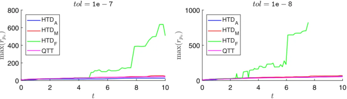
FIGURE 2 Maximum ranks of solution vectors for the metabolite synthesis model with d = 4. HTD = hierarchical Tucker decomposition; QTT = quantized TT 0 10 20 30 40 50 0 50 100 150 HTDA HTDM HTDF QTT 0 10 20 30 40 50 0 20 40 60 80 HTDA HTDM HTD F QTT
FIGURE 3 Maximum ranks of solution vectors for the extended toggle switch model with d = 4. HTD = hierarchical Tucker decomposition; QTT = quantized TT
provides the maximum relative error in the computation of the mean, assuming that simulation is at least as accurate as BDF5.
We present the numerical results in Tables 2, 4, 6, and 8 and the maximum ranks of solution vectors in Figures 2–5. The first four columns of the tables give the solver name, the accuracy tolerance tol, the time tefor which the last solution
vector is computed by 1,000 s, and the number of time steps Netaken by the computation. Column maxn(|n|) lists the
maximum truncated state space size used through the computation, column maxn(rpn)lists the maximum of the ranks of solution vectors, and column maxn(rQn)lists the maximum rank associated with the QTT approximation of the truncated generated matrix. We remark that maxn(|n|) corresponds to the maximum core tensor dimension associated with Qn
raised to the power of 2 for the QTT-based solver. Column “It” reports the average number of Jacobi iterations per time step for HTD-based solvers and the average number of DMRG iterations per time step for the QTT-based solver. Columns nnz and “Time” give the number of floating-point array elements allocated and the execution time in seconds, respectively. The next two columns report BDF5 and state space truncation errors, where
tte = Ne ∑ n=1 lten and Δp = Ne ∑ n=1 |pne − pn−1e|.
Finally, the last column reports the relative error, re𝜇, in the computation with respect to the simulation if the solution at time tfcan be computed by 1,000 s. The values under columns maxn(|n|), nnz, tte, Δp, and re𝜇are rounded to one
decimal digit of accuracy and reported using scientific notation.
The maximum truncated state space size, maxn(|n|), is an important measure for the HTD format to see the advantage
of the compact representation over the flat representation. BDF5 with the Jacobi method needs nine vectors as long as the truncated state space size (six backward difference vectors and three auxiliary vectors to store the solution, prediction, and diagonal vectors). Hence, the number of nonzeros allocated in BDF5 with flat vectors would be roughly nine times that of maxn(|n|). Note that maxn(|n|) for the QTT-based solver can be misleading in this respect. Because |n,h| does
not need to be a power of 2 for n = 1, … , Neand h = 1, … , d, the values of maxn(|n|) for the QTT format end up being
much larger than their counterparts for the HTD format.
We remark due to an earlier result that the state space truncation error at each step will be bounded by the total proba-bility mass outsidenif the truncated system is solved exactly (see theorem 2 in the work of Munsky et al.13). However,
0 2 4 6 8 10 0 200 400 600 800 HTD A HTDM HTD F QTT 0 2 4 6 8 10 0 500 1000 HTD A HTDM HTD F QTT
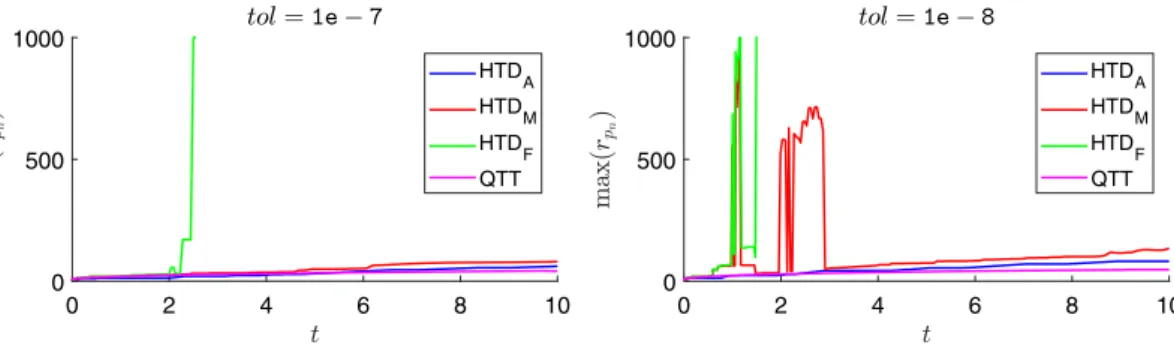
FIGURE 4 Maximum ranks of solution vectors for the lambda phage model with d = 5. HTD = hierarchical Tucker decomposition; QTT = quantized TT 0 2 4 6 8 10 0 100 200 300 400 500 HTDA HTD M HTDF QTT 0 2 4 6 8 10 0 200 400 600 800 HTDA HTD M HTDF QTT
FIGURE 5 Maximum ranks of solution vectors for the cascade model with d = 6. HTD = hierarchical Tucker decomposition; QTT = quantized TT
this value appears to be negative in some models due to numerical errors (see, for instance, the work of Kazeev et al.43).
Therefore, instead of computing the probability mass outsidenat the end of execution, we report Δp as the state space
truncation error. Note that the local state space truncation error at time step n, that is,|pne − pn−1e|, is dominated by
other numerical errors such as the BDFk truncation error if the probability mass outsiden−1andnis sufficiently large.
Hence, Δp is in fact an upper bound on the numerical error in the computed result in 1-norm upon the stopping of the execution of the solver. We therefore refer to Δp throughout the discussion as the accuracy of the CME solver. Numerical results also validate this interpretation because Δp and re𝜇are close to each other when simulation is at least as accurate as the CME solver.
We remark that the QTT-based solver achieves a higher accuracy in terms of Δp than HTD-based solvers for the same value of tol, and the ratios of tte and Δp are different for HTD- and QTT-based solvers. This phenomenon seems to be due to the structure of QTT and the method chosen to solve the linear system in BDFk, and it may be the subject of future research. Now, we discuss the models used in the numerical experiments and their particular results.
4.3
Results of models
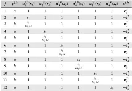
Model 1. (Metabolite synthesis)
A biological process associated with metabolite synthesis involving two metabolites and two enzymes is considered.55,68In this model, molecules interact through the nine transition classes given in Table 1. Metabolites S
1
and S2are synthesized respectively by enzymes S3and S4through the first two transition classes. The third transition
class corresponds to the consumption of metabolites, and the metabolites are degraded through the fourth and fifth transition classes. The last four transition classes correspond to the production and destruction of enzymes S3and S4.
Here, d = 4, s = (s1, s2, s3, s4), J = 9, and kA, kB, KI, k2,𝜇, KR, kEA, kEB ∈R>0.
In the numerical experiments, we let (kA, kB, KI, k2, 𝜇, KR, kEA, kEB) = (0.3, 0.3, 60, 0.001, 0.002, 30, 0.02, 0.02)
68 for
initial state s0 = (10, 10, 10, 10) and final time tf = 10. Simulation yields mean values with an accuracy of 3e−5 in
898 s. Table 2 presents the numerical results for the metabolite synthesis model.
Among the HTD-based solvers, HTDF fails to compute the solution at time tf because fixed rank control in the
Newton–Schulz method results in solution vectors with large ranks. Time and memory requirements decrease signif-icantly when adaptive rank control is used in Newton–Schulz method instead of fixed rank control. When adaptive
TABLE 1 Transition classes of the metabolite synthesis model with d = 4 j 𝜸( j) 𝜶(j) 𝟏 (s𝟏) 𝜶 (j) 𝟐 (s𝟐) 𝜶 (j) 𝟑 (s𝟑) 𝜶 (j) 𝟒 (s𝟒) v( j) 1 kAKI s 1 1+KI 1 s3 1 eT1 2 kBKI 1 s 1 2+KI 1 s4 eT2 3 k2 s1 s2 1 1 (−e1−e2)T 4 𝜇 s1 1 1 1 −eT1 5 𝜇 1 s2 1 1 −eT2 6 kEAKR 1 s1+KR 1 1 1 eT 3 7 kEBKR 1 1 s2+KR 1 1 eT 4 8 𝜇 1 1 s3 1 −eT3 9 𝜇 1 1 1 s4 −eT4
TABLE 2 Numerical results for the metabolite synthesis model with d = 4
Solver tol te Ne maxn(|n|) maxn(rpn) maxn(rQn) It nnz Time tte Δp re𝝁
HTDA 1e−6 10.00 205 3e5 21 N/A 1.5 7e4 7 1e−4 2e−3 2e−3
HTDM 10.00 221 3e5 30 N/A 1.3 8e4 8 1e−4 3e−3 3e−3
HTDF 5.84 167 2e5 656 N/A 1.4 1e8 1,491 8e−5 1e−3 –
QTT 10.00 151 1e8 33 13 2.3 2e6 69 5e−5 3e−5 2e−5
HTDA 1e−7 10.00 223 5e5 60 N/A 1.9 2e5 33 9e−6 1e−4 1e−4
HTDM 10.00 227 5e5 79 N/A 1.5 4e5 41 1e−5 1e−4 1e−4
HTDF 2.55 161 1e5 1,000 N/A 1.3 8e7 1,075 6e−6 4e−5 –
QTT 10.00 215 1e8 42 13 2.3 3e6 200 7e−6 5e−6 1e−5
HTDA 1e−8 10.00 314 7e5 81 N/A 1.9 6e5 144 1e−6 2e−5 2e−5
HTDM 10.00 306 7e5 960 N/A 1.5 8e6 581 1e−6 2e−5 2e−5
HTDF 1.52 178 1e5 1,000 N/A 1.5 6e7 1,240 8e−7 2e−6 –
QTT 10.00 303 1e8 47 14 2.2 6e6 469 1e−6 7e−7 1e−5
Note.HTD = hierarchical Tucker decomposition; QTT = quantized TT.
rank control is also used in the Jacobi method, improvements in time and memory become as high as 75% and 92% for tol = 1e−8, respectively.
Figure 2 shows that the maximum rank of solution vectors changes smoothly over time when HTDAis used.
Regard-ing the QTT format, the maximum rank associated with the approximation of Qnis modest, and the maximum rank
associated with solution vectors turns out to be the best among all solvers for decreasing values of tol.
Memory requirements of the QTT-based solver are at least an order of magnitude higher than those of solvers using HTDA and HTDM. Note that the number of nonzeros allocated for flat vectors would roughly be
22≈(9×5e5/23e55)and 10≈(9×7e5/6e5) times that of compact vectors allocated in HTDAfor accuracy
toler-ances of 1e−7 and 1e−8, respectively. Furthermore, the QTT-based solver is clearly slower than the HTDA-based
solver, although the discrepancy becomes relatively smaller as tol decreases. On the other hand, the accuracy of the QTT-based solver is higher than those of HTD-based solvers for all values of tol. We remark that when tol =1e−8, the accuracy of simulation is reached by HTDAand HTDM. The QTT-based solver reaches the same accuracy early on,
when tol =1e−6.
Model 2. (Extended toggle switch)
A system of stochastic chemical kinetics modeling the biological process associated with a toggle switch is considered.28 In this model, S
1 and S2 are two mutually repressing gene products and express the proteins S3 and S4, respectively. These four molecules interact through the eight transition classes given in Table 3. The first four
transition classes correspond respectively to the production of S1, the production of S2, the destruction of S1, and the
destruction of S2. The fifth and sixth transition classes correspond to the expression of gene products, and the last two
transition classes correspond to the destruction of gene products. Here, d = 4, s = (s1, s2, s3, s4), J = 8, and a11, a12, a21, a22, a3, a4, a5, a6, a7, a8∈R>0.
TABLE 3 Transition classes of the extended toggle switch model with d = 4
j 𝜸( j) 𝜶(j) 1 (s𝟏) 𝛂 (j) 𝟐 (s𝟐) 𝜶 (j) 𝟑 (s3) 𝜶(𝟒j)(s𝟒) v( j) 1 a11 1 s21 2+a12 1 1 eT 1 2 a21 s21 1+a22 1 1 1 e T 2 3 a3 s1 1 1 1 −eT1 4 a4 1 s2 1 1 −eT2 5 a5 s1 1 1 1 eT3 6 a6 1 s2 1 1 eT4 7 a7 1 1 s3 1 −eT3 8 a8 1 1 1 s4 −eT4
TABLE 4 Numerical results for the extended toggle switch model with d = 4
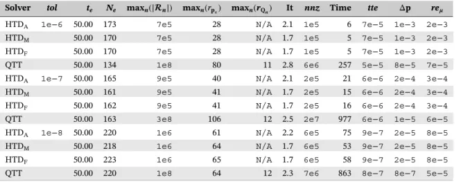
Solver tol te Ne maxn(|n|) maxn(rpn) maxn(rQn) It nnz Time tte Δp re𝝁
HTDA 1e−6 50.00 173 7e5 28 N/A 2.1 1e5 6 7e−5 1e−3 2e−3
HTDM 50.00 170 7e5 28 N/A 1.7 1e5 5 7e−5 1e−3 2e−3
HTDF 50.00 170 7e5 28 N/A 1.7 1e5 5 7e−5 1e−3 2e−3
QTT 50.00 134 1e8 80 11 2.8 6e6 257 5e−5 8e−5 7e−5
HTDA 1e−7 50.00 165 9e5 40 N/A 2.1 2e5 21 6e−6 2e−4 3e−4
HTDM 50.00 161 9e5 41 N/A 1.7 2e5 15 6e−6 2e−4 3e−4
HTDF 50.00 162 9e5 41 N/A 1.7 2e5 16 6e−6 2e−4 3e−4
QTT 50.00 163 3e8 106 12 2.5 2e7 977 6e−6 1e−5 6e−5
HTDA 1e−8 50.00 220 1e6 61 N/A 2.2 6e5 75 9e−7 2e−5 8e−5
HTDM 50.00 218 1e6 64 N/A 1.7 6e5 53 9e−7 2e−5 8e−5
HTDF 50.00 223 1e6 65 N/A 1.7 6e5 58 9e−7 2e−5 8e−5
QTT 50.00 220 1e8 64 12 2.3 7e6 863 8e−7 8e−7 5e−5
Note.HTD = hierarchical Tucker decomposition; QTT = quantized TT.
In the numerical experiments, we let
(a11, a12, a21, a22, a3, a4, a5, a6, a7, a8) = (10, 30, 10, 30, 0.017, 0.017, 0.01, 0.01, 0.01, 0.01)28
for initial state s0= (10, 10, 10, 10) and final time tf=50. Simulation yields mean values with an accuracy of 7e−5 in
726 s. Table 4 presents the numerical results for the extended toggle switch model.
In this model, rank control strategies for HTD-based solvers do not influence the maximum ranks of solution vectors much (see Figure 3). Adaptive rank control in the Jacobi method increases the average number of iterations it performs due to additional iterations that get executed after rank bounds are increased. However, this increase is not offset by a sizable (if any) decrease in the ranks of solution vectors. Consequently, HTDAends up being slower than the other
HTD-based solvers. Regarding the QTT format, ranks associated with the approximation of Qn are again modest;
however, the maximum rank associated with solution vectors turns out to be the largest among all solvers except for
tol =1e − 8.
The QTT-based solver is more accurate than HTD-based solvers for the same value of tol in this model as well. The accuracy of simulation is reached by HTD-based solvers when tol = 1e − 8 and by the QTT-based solver for all values of tol used. However, compared with HTD-based solvers, the QTT-based solver requires about an order of magnitude more memory and significantly more time to compute the solution as accurately as simulation computes mean values. The number of nonzeros allocated for flat vectors would roughly be 40 and 15 times that of compact vectors allocated in HTD format for accuracy tolerances of 1e−7 and 1e−8, respectively.
Model 3. (Lambda phage)
The biological process associated with the life cycle of bacteriophage-𝜆 is a naturally occurring toggle switch that consists of two phases.23,32,69Transition from one phase to the other is controlled by competing proteins S1and S2. In
this model, molecules interact through 10 transition classes given in Table 5. Proteins S1and S2are generated through