Inventory management problem for two substitutable products : a bayesian approach

INVENTORY MANAGEMENT PROBLEM

FOR TWO SUBSTITUTABLE PRODUCTS: A

BAYESIAN APPROACH

a thesis submitted to

the graduate school of engineering and science

of bilkent university

in partial fulfillment of the requirements for

the degree of

master of science

in

industrial engineering

By

Burcu Tekin

July 2016

INVENTORY MANAGEMENT PROBLEM FOR TWO SUBSTI-TUTABLE PRODUCTS: A BAYESIAN APPROACH

By Burcu Tekin July 2016

We certify that we have read this thesis and that in our opinion it is fully adequate, in scope and in quality, as a thesis for the degree of Master of Science.

¨

Ulk¨u G¨urler(Advisor)

¨

Ozlem C¸ avu¸s ˙Iyig¨un

Ayhan ¨Ozg¨ur Toy

Approved for the Graduate School of Engineering and Science:

Levent Onural

ABSTRACT

INVENTORY MANAGEMENT PROBLEM FOR TWO

SUBSTITUTABLE PRODUCTS: A BAYESIAN

APPROACH

Burcu Tekin

M.S. in Industrial Engineering Advisor: ¨Ulk¨u G¨urler

July 2016

Accurate estimation of demand and the inventory levels are must for customer satisfaction and the profitability of a business. In this thesis, we consider two main topics: First, the joint estimation of the demand arrival rate, primary and substitute demand rates in a lost sales environment with two products is provided using a Bayesian methodology. It is assumed that demand arrivals for the products follow a Poisson process where the unknown arrival rate is a random variable. An arriving customer requests one of the two products with a certain probability and may substitute the other product if the primary demand is not available. We consider a general mixture gamma density for prior of the Poisson arrival rate and a general prior for the joint distribution of the primary and substitute demand probabilities. It is observed that the resulting marginal posterior and the conditional posterior density of demand arrival rate given the other parameters, after observation of n-period data, are again in the structure of gamma mixtures. Then, we calculated the inventory levels of the products dynamically with the help of first part. Using the updated posterior demand rates on the observed data from the previous period, we revised the inventory levels for the following period to maximize the profit. Finally, some numerical results for both parts are presented to illustrate the performance of the estimations.

Keywords: Inventory Management, Bayesian Estimation, Substitution, Poisson Demand, Lost Sales.

¨

OZET

˙IKAME ED˙ILEB˙IL˙IR ˙IK˙I ¨

UR ¨

UNL ¨

U B˙IR ENVANTER

PROBLEM˙IN˙IN BAYES YAKLAS

¸IMI ˙ILE Y ¨

ONET˙IM˙I

Burcu Tekin

End¨ustri M¨uhendisli˘gi, Y¨uksek Lisans Tez Danı¸smanı: ¨Ulk¨u G¨urler

Temmuz 2016

Talep ve envanter seviyelerinin do˘gru tahmini m¨u¸steri memnuniyeti ve i¸sletmenin karlılı˘gı a¸cısından olmazsa olmazdır. Bu ama¸cla, iki ana ba¸slık ¨uzerinde ¸calı¸sılmı¸stır. ˙Ilk olarak, kayıp satı¸sın oldu˘gu iki ¨ur¨unl¨u bir ortamda talep geli¸s oranları, birincil talep oranları ve ikame talep oranları i¸cin Bayes metodolo-jisi kullanılarak b¨ut¨unle¸sik bir tahmin y¨ontemi sunulmu¸stur. Taleplerin Pois-son da˘gılım ile geldi˘gi ve geli¸s oranının bilinmeyen bir rassal de˘gi¸sken oldu˘gu varsayılmı¸stır. Gelen m¨u¸steriler belli bir olasılıkla ¨ur¨unlerden birini tercih et-mekte, ilk tercihi yoksa ba¸ska bir olasılıkla di˘ger ¨ur¨un¨u almakta ya da hi¸cbir ¸sey almadan d¨onmektedir. Poisson geli¸s oranı i¸cin ¨onsel da˘gılım olarak Genel Gama Bile¸simi Da˘gılımı, birincil talep oranları ve ikame talep oranları i¸cin ise ¨

ozellikle belirtilmemi¸s da˘gılımlar se¸cilmi¸stir. N-g¨ozlem d¨onemi boyunca veri top-landıktan sonra, marjinal ve ko¸sullu sonraki da˘gılımların yine Gama Bile¸simi for-munda oldu˘gu g¨ozlemlenmi¸stir. ˙Ikinci kısımda, envanter seviyeleri ilk kısımdaki y¨ontemler kullanılarak dinamik olarak hesaplanmı¸stır. G¨uncellenmi¸s sonraki talep oranları ve g¨ozlemlenen veriler kullanılarak bir sonraki d¨onem i¸cin karı en y¨uksek seviyeye ta¸sıyan envanter seviyeleri bulunmu¸stur. Son olarak, her iki ana ba¸slık i¸cin de sayısal analizler ve hesaplamalar sunulmu¸stur. B¨oylelikle sunulan teorilerin performansı g¨ozlenebilmi¸stir.

Anahtar s¨ozc¨ukler : Envanter Y¨onetimi, Bayesyen Tahmin, ˙Ikame Etme, Poisson Talep, Kayıp Satı¸s.

Acknowledgement

I would like to express my appreciation to my adviser Prof. Dr. ¨Ulk¨u G¨urler for her support, guidance, encouragement and help throughout this study. Her invaluable advices and experiences about the life will always be on my mind. Working under her supervision was always a pleasure for me.

I would like to thank Assist. Prof. Dr. ¨Ozlem C¸ avu¸s ˙Iyig¨un and Assoc. Prof. Dr. ¨Ozg¨ur Toy for accepting to read and review this thesis and their valuable comments and guidance.

I wish to thank Assoc. Prof. Dr. Emre Berk for his substantial suggestions throughout this study.

I would like to thank my dearest friend Nihal Berkta¸s for her joy, love and support on every subject during these last four years. I wish to thank my of-fice mates ¨Oz¨um Korkmaz, Nil Karacao˘glu, Merve Meraklı, H¨useyin G¨urkan and O˘guz C¸ etin for their precious friendship, and providing a great, joyful work en-vironment.

I also would like to thank Fulya Sudur Zalluho˘glu, M¨uge Akkavak and Cansu Alakbarova for their endless support and being always like a sister for me.

Above all, I am deeply grateful to to my mother Sevtap Tekin, my father ¨Ozg¨ur Tekin and my brother Muharrem Eren Tekin for their endless support, patience and love throughout my life. Their love and support is always a strength to me in every moment of my life. I feel very lucky to have such a wonderful family.

Contents

1 Introduction 1

2 Literature Review 5

2.1 Non-Bayesian Perspective . . . 5 2.2 Bayesian Approach . . . 7 2.3 Substitution Based Inventory Management . . . 8

3 Preliminaries 11

3.1 Bayesian Estimation . . . 11 3.2 Model Description . . . 14

4 Joint Estimation of Primary and Substitute Demand Parameters 16 4.1 First Period Analysis . . . 18 4.2 Multiple Period Analysis . . . 23 4.3 Special Case 1: Base Demand Rate Estimation . . . 25

CONTENTS vii

4.4 Special Case 2: Substitute Demand Rate Estimation . . . 26

5 Dynamic Estimation of Stock Levels 29

5.1 Computation of Expected Profit . . . 30 5.1.1 Single Period Analysis . . . 30 5.2 Dynamic Update of Inventory Levels . . . 32

6 Numerical Study 34

6.1 Parameter Sensitivity in Base Demand Rate Estimation . . . 35 6.1.1 Priority Sensitivity . . . 35 6.1.2 Initial Inventory Levels . . . 41 6.1.3 Impact of Substitution on Estimation of Demand Rate . . 47 6.2 Dynamic Estimation of Stock Levels . . . 51 6.2.1 Computation of Profit Maximizing Inventory Levels . . . . 51 6.2.2 The Effect of Different Substitution Probabilities . . . 61 6.2.3 The Effect of Different Prior Selections . . . 67

7 Conclusion 83

List of Figures

6.1 Prior Distribution Graph of η0 = [2; 10], θ0 = [5; 4] for different c0

values . . . 36 6.2 Prior Distribution Graph of η0 = [20; 10], θ0 = [6; 7] for different c0

values . . . 37 6.3 Mean of posterior demand distributions over time for 5 different

realizations where η0 = [2; 10], θ0 = [5; 4] . . . 38

6.4 Mean of posterior demand distributions over time for the initial inventory levels SA= SB = M ean . . . 42

6.5 Mean of posterior demand distributions over time for the initial inventory levels SA= SB = M ean + σ . . . 43

6.6 Mean of posterior demand distributions over time for the initial inventory levels SA= SB = M ean − σ . . . 44

6.7 Mean of posterior demand distributions over time for the initial inventory levels SA= SB = M ean + 2σ . . . 45

6.8 Mean of posterior demand distributions over time for the initial inventory levels SA= SB = M ean − 2σ . . . 46

LIST OF FIGURES ix

6.9 Prior Distribution Graph of η0 = [20; 10], θ0 = [6; 7] for different c0

values . . . 47 6.10 Change in the Posterior Mean over Period when there is no

substitution(α = β = 0) . . . 48 6.11 Change in the Posterior Mean over Period when α = β = 0.3 and

α = β = 0.5 . . . 49 6.12 Change in the Posterior Mean over Period when α = β = 0.7 and

α = β = 1 . . . 50 6.13 Change in the Profit Maximizing Inventory Levels over 40 Review

Periods for Simulation Realization 3 . . . 52 6.14 Change in the Profit Maximizing Inventory Levels over Review

Periods for Three Different Simulation Realizations . . . 56 6.15 Expected Profit Values for Dynamically Calculated vs. Constant

(S₀∗) Inventory Levels for Three Different Simulation Realizations 57

6.16 Expected Profit Values for Different Initial Inventory Level Policies for Three Different Simulation Realizations . . . 58 6.17 Absolute Difference from the Maximum Profit Level for Constant

Inventory Level Policies for Three Different Simulation Realizations 59 6.18 Profit Maximizing Inventory Levels for α = β = 0, 0.4, and 1 over

time, Simulation Realization 1 . . . 62 6.19 Change in the Expected Maximum Profit with Updated Stock

Lev-els, for α = β = 0, 0.4, and 1 over time, Simulation Realization 1 . 63 6.20 Expected Profit Levels for Different Inventory Level Policies, where

LIST OF FIGURES x

6.21 Change in the Profit Maximizing Inventory Levels for η0 = [2; 10],

θ0 = [5; 4] and c0 = [0.9; 0.1] . . . 68

6.22 Change in the Profit Maximizing Inventory Levels for η0 = [2; 10],

θ0 = [5; 4] with c0 = [0.4; 0.6] and c0 = [0.9; 0.1] . . . 69

6.23 Expected Maximum Profit Values for η0 = [2; 10], θ0 = [5; 4] with

c0 = [0.4; 0.6] and c0 = [0.9; 0.1] . . . 70

6.24 Change in the Profit Maximizing Inventory Levels for η0 = [20; 10],

θ0 = [6; 7] and c0 = [0.9; 0.1] . . . 71

6.25 Change in the Profit Maximizing Inventory Levels for η0 = [2; 10],

θ0 = [5; 4], c0 = [0.4; 0.6] and η0 = [20; 10], θ0 = [6; 7], c0 = [0.9; 0.1] 73

6.26 Expected Maximum Profit Values for η0 = [2; 10], θ0 = [5; 4], c0 =

[0.4; 0.6] and η0 = [20; 10], θ0 = [6; 7], c0 = [0.9; 0.1] . . . 74

6.27 Prior Distribution Graph of η0 = [5; 10], θ0 = [3; 6] for different c0

values . . . 76 6.28 Change in the Profit Maximizing Inventory Levels for η0 = [2; 10],

θ0 = [5; 4], c0 = [0.4; 0.6] and η0 = [5; 10], θ0 = [3; 6] and c0 =

[0.4; 0.6] . . . 77 6.29 Expected Maximum Profit Values for η0 = [2; 10], θ0 = [5; 4], c0 =

[0.4; 0.6] and η0 = [5; 10], θ0 = [3; 6] and c0 = [0.4; 0.6] . . . 78

6.30 Prior Distribution Graph of η0 = [2; 2.5], θ0 = [5; 1] for different c0

values . . . 80 6.31 Change in the Profit Maximizing Inventory Levels for η0 = [2; 10],

θ0 = [5; 4], c0 = [0.4; 0.6] and η0 = [2; 2.5], θ0 = [5; 1] and c0 =

LIST OF FIGURES xi

6.32 Expected Maximum Profit Values for η0 = [2; 10], θ0 = [5; 4], c0 =

List of Tables

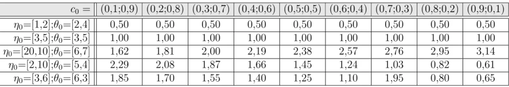
6.1 Prior Mean Values for Different Parameter Sets of Prior Distribution 39 6.2 CM AD0 Values for Different Realizations and c0 values, where

η0 = [2; 10], θ0 = [5; 4] . . . 39

6.3 CMAD’ Values for Different Realizations and c0 values, where η0 =

[2; 10], θ0 = [5; 4] . . . 40

6.4 Updated Demand Values, Inventory Levels and Maximum Ex-pected Profit for Simulation Realization 1 . . . 53 6.5 Updated Demand Values, Inventory Levels and Maximum

Ex-pected Profit for Simulation Realization 2 . . . 53 6.6 Updated Demand Values, Inventory Levels and Maximum

Ex-pected Profit for Simulation Realization 3 . . . 53 6.7 Absolute Sum of the Differences from the Maximum Profit Levels

for Constant Inventory Levels . . . 60 6.8 Total Profit of all periods for Constant Inventory Levels . . . 60 6.9 Expected Maximum Profit Values for Different Substitution Rates 64 6.10 Total Profit of all periods for Different Inventory Policies . . . 65

Chapter 1

Introduction

In the past, main stages of a supply chain, that are procurement, production and distribution, are managed independently by keeping huge buffer stocks. However, competitive business environment forces firms to built agile supply chains which quickly respond to variable demand. To stay in the competition, firms need to decrease operation and inventory holding costs while ensuring the customer satisfaction.

Uncertainties emerged by the factors, such as customer demand, product qual-ity or competition, constitutes risk in supply chains. To reduce the risk, retailers intend to order more than they need. An accurate forecast for the future demand is crucial for a firm to manage inventories and actual sales in a successful man-ner. Both reduction in out-of-stocks and the improvement in on-shelf availability basically depend on this ability. However, decreasing product lifetimes, competi-tive promotions that effect purchase decisions, proliferation in product types and the substitutions emerged in cases of stock-outs make an accurate estimation of demand more difficult than the past.

The substitution behavior of customers particularly presents the greatest chal-lenge for practitioners. Predicting the customer response in case of not finding the desired product, is really important for the retailers. In this case, there are

four possible actions: the customer may postpone buying, decide not to purchase the product, purchase the product from another retailer, or substitute the prod-uct with another item [1]. A study by Gruen et al. [2] states that 40 percent of customers who are faced with a stock-out situation, buy a substitute product instead.

If a product is not in the portfolio of the retailer, or, although it is in the port-folio, it has stock-out, customers’ primary demand cannot be satisfied. Although both may lead to substitution of the product, the first one is a business decision. However, the second case is caused by demand uncertainty and the inventory de-cisions. In [3], it is stated that 8.3 percent of the stock keeping units that a retailer has are out-of-stock at a particular moment in time. Therefore, understanding the substitution behavior and adopting the inventory policies accordingly are of significant importance to the firms.

Although, using accurate demand and substitution information is crucial for management of inventory systems, estimation of demand and substitution rates in a multi-product environment is not that easy. The methodologies developed for single item settings are not directly applicable; product substitution sometimes confounds observations; and, new synchronized information such as item-specific stock-out times are needed for these settings. For example, consider the joint es-timation of demand and substitution rates for a system with two products under a periodic review in which both items are replenished at the beginning of each pe-riod. Within a review period, stock-outs may occur until the next replenishment time, especially for fast moving items. When a stock-out occurs, the customer may prefer to buy another product if available. In such a setting, the observed sales of a product do no longer give accurate information for its primary demand since it includes the information for demand of other items when the product assortments include multiple substitutable items. If substitution behavior of the customer is not modeled properly, this may lead to identification problems from a statistical point of view. Furthermore, if the combined demand in the review period, which is the actual demand for a product and the demand transferred to this product due to the stock out of the other, exceeds the available stock available at the beginning of a period, then a well known type of incomplete

data, namely censored data is observed, which has to be explicitly taken into ac-count for reliable estimates of demand. Thus, aside from resulting in possible lost sales cost and intangibles such as loss of customer trust or erosion of reputation, product substitution results in possible information loss as well.

In this thesis, we provide an inventory management policy using Bayesian approach for the joint estimation of total demand rate, primary and substitute purchase probabilities.We consider a setting of two-products with unit Poisson customer arrivals. Advantage of the Bayesian estimation methodology lies in gathering the prior information available about the parameters with the data re-vealed over time. For the Poisson arrival rate, we consider a prior distribution expressed as a general mixture of gamma densities and the joint prior distribution of the primary and substitute demands is left general. It is initially assumed that the arrival rate is independent of the primary demand and substitution probabili-ties. The joint posterior densities are obtained after n-periods of observation. We establish the result that the posterior conditional density of the Poisson arrivals also follow a mixture of gamma densities with parameters modified with respect to the observed data. On the other hand, the marginal joint posterior of the demand and substitution probabilities keep the general form. We also consider a special case of practical interest: the estimation problem for the demand rate when the primary demand and substitution probabilities are known. The case is applicable to the situations where the products are introduced to new markets where the demand rate is unknown due to the particulars of the new market but the substitution behavior may be more apparent from the consumer behav-ior in the existing markets. Another special case may be where demand rate is known but substitution probabilities are not known. This case may reflect the environments where new products are launched to the market for which market-ing research might reveal reliable estimates for the demand size but the effect of substitution may not be that obvious.

Using the results of demand rate estimation, we have developed an algorithm which dynamically updates the initial inventory levels at the begging of each period. Main aim in this section was no different than the goal of every firm: profit maximization. We introduced the costs of substitution, inventory carrying

and the lost sales, than try to maximize the profit by updating the inventory levels with revealed data from the prior observations. In our study we incorporate the accumulated data to estimate the unknown distributions of demand rate using a Bayesian perspective. This approach allows the decision makers to use information that become dynamically available in an efficient way. Despite the complexity of functional forms, the Bayesian approach provides a convenient tool for updating the demand estimation by taking into account the dynamic nature of the available data.

The performance of the suggested estimators are evaluated by simulating sev-eral realizations and observing the dynamic behavior of the estimators. Our numerical results show that the estimates converge to the target values of the de-mand parameters after sufficient data has accumulated. Also, parameter analysis are conducted to obverse the effect on the accuracy of our estimation. Finally, another numerical study is provided to evaluate performance of the provided algorithm for the dynamic inventory update policy.

The rest of this thesis is organized as follows. In Chapter 2, we have introduced the literature about inventory management and demand estimation in three main categories, namely; non-Bayesian Perspective, Bayesian Approach and substitu-tion based inventory management. In Chapter 3, preliminaries of the study is provided. We begin with a general description of the Bayesian Estimation.Then, we mentioned about the specifications and essentials of our model setting. In Chapter 4, joint estimation of the primary and substitute demand parameters are formulated. Single period calculations are presented. Then, generalization for multiple period analysis is provided. Finally, base demand rate estimation is studied as a special case. In Chapter 5, we have used the theory provided in Chapter 4 to determine profit maximizing inventory levels. With the help of es-timated demand rates, inventory levels for the next period is updated to increase the profit. In Chapter 6, numerical studies are provided for both of the theories mentioned in Chapter 4 and 5. Parameter analysis and numerical computations are conducted and the results are evaluated with different key performance indi-cators. Finally, in Chapter 7 we give the concluding remarks.

Chapter 2

Literature Review

In this section we provide our findings in the literature about the inventory man-agement under three categories named as non-Bayesian perspective, Bayesian Approach and substitution based inventory management.

2.1

Non-Bayesian Perspective

Regarding demand estimation in the inventory theory literature, there are two basic approaches; namely, the frequentist and the Bayesian.

In the frequentist perspective, Nahmias [4] is the first to analyze the censored demand case with normally distributed demand. Agrawal and Smith [5] then considered the estimation of negative binomial demand, in the presence of cen-soring induced by lost sales. Anupindi et al. [6] tackle this problem for a vending machine environment and propose maximum likelihood estimation for demand rate under stock-outs. They analyze the results based on both perpetual and periodic system data. Although vending machines provide a good example, the model under study is general enough to include any duopoly market with two major product (such as soft-drinks or chocolate brands etc.), or problems with single item two locations (such as cash-machines of the same bank located close

enough to allow for substitution in heavy population areas).

Demand estimation and assortment optimization under substitution are stud-ied by Kok and Fisher [7]. Their work focuses on an assortment planning model based on product substitution. The authors propose a procedure for estimating the parameters of demand and the substitution rate for various products includ-ing the ones that are new on the market. Karabati et al. [3] present a method to estimate stock-out-based substitution rates by using point-of-sale data.

In another recent work, Conlon and Mortimer [8] investigate the demand es-timation problem under incomplete product availability in the vending industry. They specifically address the bias in demand parameter estimates and propose a method to correct the bias by allowing for changes in product availability un-der a periodical inventory review. In the proposed model they assess an EM (expectation maximization) algorithm as well as a Bayesian approach to handle missing data. The results demonstrate significant differences in demand estimates reflecting significant impact of stock-outs on profitability.

Musalem et al. [9] develop a demand model that takes into account the effect of stock outs on customer choice. The model is based on utility maximization principles and is estimated using sales data from multiple stores.

Vulcano et al. [10] consider estimating demand for substitutable products from sales transaction data. They employ the expectation maximization method and discrete choice models using the sales and product availability data, and illustrate the effectiveness of the proposed method using real as well as simulated data sets. Huh, Levi and Orlin [11] use the well-known nonparametric Kaplan-Meier estimator for censored data from statistics, to propose a new class of adaptive data-driven inventory control policies when the demand distribution is not known and only the sales data are available. Finally, Kok et al. [12] provides a wide range of other related works in the literature.

2.2

Bayesian Approach

The Bayesian perspective for demand estimation has been adopted by several authors, starting with the early work of Scarf [13, 14] and Iglehart [15]. Later, Azoury [16], Lovejoy [17], Bradford and Sugrue [18], Hill [19, 20] and Eppen and Iyer [21] considered various aspects of inventory management with Bayesian updating of demand distributions.

Lariviere and Porteus [22] considered Bayesian updating with partially ob-served sales, Ding et al. [23] considered the censored demand setting for a per-ishable product and examined optimal stocking decisions.

Berk, G¨urler and Levine [24] revisited the problem when lost demands are not observed and proposed an approximate methodology retaining the conjugacy properties of priors.

Kamath and Pakkala [25] compare Bayesian and non-Bayesian approaches to demand estimation under both stationary and non-stationary demand. It is ob-served that ignoring prior information could be very costly especially in the case of variable demand rate. The paper strongly recommends considering the Bayesian approach when there is a high uncertainty about the demand.

Chen and Plambeck [26] revisited the periodic review lost sales inventory prob-lem and incorporating the learning about the probability of substitution they show that substitution reduces the Bayesian optimal inventory level in the case that lost sales are observed. They state that reducing the inventory level has two beneficial effects: to observe and learn more about customer substitution behav-ior and (for a nonperishable product) to reduce the probability of overstocking in subsequent periods.

Yelland [27] compared the forecast performance of three different state-space models, using Bayesian methods.

2.3

Substitution Based Inventory Management

The practical need for demand estimation in the presence of product substitution is best illustrated by the extensive project conducted by Gruen et al. [2]. This study has revealed that the average out-of-stocks was 8.3 per cent worldwide and that, in the case of a stock-out, customer response may be buying the same item elsewhere (31 per cent), substituting a different brand (26 per cent), substituting the same brand (19 per cent), delaying the purchase (15 per cent) or not purchas-ing at all (9 per cent). The same study points out that substitution rates vary significantly from one stock-keeping-unit (SKU) category to another, and that the erroneous store forecasting accounts for 13 per cent of the causes for out of stock, overall worldwide sales losses range from 3.7 to 4.0 per cent, whereas category sales losses vary from 2.1 to 4.5 per cent with more than two-fold difference.

The important role that the presence of substitution among products plays on the stocking decisions and ensuing costs has been well established in the inventory theoretic literature. In one of the earliest works, Ignall and Veinott [28] showed that the optimality of a myopic inventory control policy depends on specific con-ditions in a periodic review setting. In a single period operating environment with downward substitution among products, Bassok et al. [29] illustrated the benefits of taking substitution effects explicitly into consideration for optimal or-dering quantities and showed that a greedy allocation policy is optimal. Smith and Agrawal [30] demonstrated the impact of substitution for assortment plan-ning and determination of optimal stocking levels using actual retail sales data described by a negative binomial demand distribution. Ernst and Kamrad [31] supported their analysis of an inventory system with two substitutable products by using sales data explicitly during stock-out occasions. Also for two-product settings, Honhon et al. [32] and G¨urler and Yilmaz [33] further illustrated the impact of substitution in single period settings. Xu et al. [34] established the optimal substitution structure for an infinite horizon periodic review system with two products in the presence of both supplier- and customer-driven substitution. Within the game theory context, Parlar [35] is among the first who considered

a game theoretic analysis of inventory problems with random demands and sub-stitutable products. In a single period setting, he showed that possible product substitution would significantly affect the optimal decisions of inventory man-agers. In the same vein, Netessine and Rudi [36] studied centralized and com-petitive inventory models with demand substitution, where unsatisfied demand for a product flow to other products in deterministic proportions. They com-pared the optimal stocking policies of substitutable products and showed that, when demand is multivariate normal, under centralized inventory management the total profit is decreasing in demand correlation. Recently, Vaagen et al. [37] demonstrated in a single-period multi-item substitutable product model that sim-plifying assumptions on distributions and dependencies can lead to rather poor solutions and profit losses. Similarly, Y¨ucel et al. [38] point out that neglecting customer-driven substitution may lead to significantly inefficient assortments.

In Shah and Avittathur [39], single period inventory planning problem with multiple items is studied in a one-way substitution environment. They considered two problems which are the selection of the optimal product portfolio and inven-tory levels with the objective of profit maximization. Two separate heuristics are proposed to solve two problems. Comparison between the heuristic solutions against the optimal solutions are provided using some numerical examples. Also, a series of sensitivity analysis are conducted to observe the impact of important parameters on retailer profits.

Nagarajan and Rajagopalan [40] considered several inventory management problems under fixed substitution rates. For single-period, two product model, closed-form expressions are provided to obtain the optimal inventory levels. Then, the result is executed on a special N-product model. A dynamic program is de-veloped for the two-product, multiple periods, and the finite-horizon case. They get the result that as substitution rate increases, optimal inventory levels will be lower.

Stavrulaki [41] demonstrated on the joint effect of demand stimulation and product substitution on inventory decisions by considering single-period, two-product setting with two way substitution. They developed two heuristics: No

Substitution Heuristic, ignores the effect of product substation and finds the optimal order quantities only considering the demand stimulation effect and No Stimulation Heuristic, ignores the effect of demand stimulation and finds the optimal order quantities only considering the product substitution effect. They evaluate the impact of varying substitution rates; critical fractile ratios; demand stimulation and variability; and correlated demands on the heuristic performance are evaluated.

Finally, Tan and Karabati [42] studied a multi-product profit maximizing com-putation method which has a service level constraint. They consider an inventory management problem with Poisson arrival processes, stock-out based dynamic demand substitution, and lost sales. They used a genetic algorithm where the expected inventory levels are estimated with the mean value approximation and expected direct and substitution sales are estimated with the two moment ap-proximation. For two product case formulation is provided.

Chapter 3

Preliminaries

Before formally introducing the Bayesian Approach for estimation of demand in a lost sales environment, we shall briefly explain the classical Bayesian Estimation methodology and our model setting.

3.1

Bayesian Estimation

The main aim of statistical inference is reaching conclusions about a phenomenon using the observed data. Presence of statistical knowledge enlightens some un-certainties involved in a decision problem. These unun-certainties can be considered as unknown numerical quantities such as vectors or matrices. Statistics is com-posed of two main point of views: the frequentist approach and the Bayesian approach. The main difference between the frequentist and Bayesian approaches is the understanding of probability.

The frequentist approach, which is also known as classical approach, interprets probability as a long-run frequency. It employs hypothesis testing and confidence intervals as two of the main ways of inference. According to frequentists , data is a repeatable random sample and the underlying parameters remain constant during this repeatable process. So, there is a frequency.

On the other hand, in Bayesian approach there is an initial belief about the probability before collecting the data. This definition of probability is usually named as subjective probability. It considers data as an observation from a realized sample. Parameters are unknown and described probabilistically. The main aim of a Bayesian analysis is getting the posterior distribution. Posterior distribution is defined as a weighted average of knowledge about the parameters before the data observed (which is represented by the prior distribution) and the information about the parameters contained in the observed data (which is represented by the likelihood function) by Glickman and Dyk [43]. When the posterior distribution is retrieved, the point and interval estimates of parameters can be computed and the prediction for future data can be made.

A typical Bayesian analysis is composed of four stages: data modeling, prior distribution selection, posterior distribution calculation and posterior distribution analysis.

The initial step for a Bayesian analysis is deciding on a probability model for the data. If the parameters are known, this step will be choosing a probability distribution for the data. It will be a conditional probability function of observed data, given the parameter set. If the observed data values are independent, say y1, ..., yn; and the unknown parameter vector is θ , then the probability function

would be p(yi|θ).

After choosing the probability model, a prior distribution for the unknown model parameters need to be declared. Prior distribution represents the cur-rent state of knowledge about the model parameters before the data is observed. While selecting the prior distribution, previous studies, opinions of the experts, or research intuitions about the data may guide one. The main point of choosing the prior distribution is representing the prior belief about the data model. When prior beliefs are available, they may be converted to moments such as mean and variance, to fit a common distribution to these moments. Different choices of prior distribution can result in different inference from the same data.

used to describe a function of a parameter vector for a given outcome. When assuming that θ is fixed, integrating the probability function over all possible values of y gives one in total. If the same function is considered when data is fixed and the parameter is the variable, it is called the likelihood. Values of θ where the likelihood is high are those that have a high probability of producing the observed data. Assume that the observed data values y = (y1, ..., yn) are

obtained, the likelihood function will be

L(θ|y) = p(y1, ..., yn|θ) =

Y

p(yi|θ)

In Bayesian analysis, likelihood function has all of the information which is ob-tained from the data about the parameter set, θ . After computing the likelihood function, Bayes’ theorem is applied to obtain the posterior distribution p(θ|y):

p(θ|y) = _R p(θ)p(θ|y) p(θ)p(y|θ)dθ =

p(θ)L(θ|y)

p(y) ∝ p(θ)L(θ|y)

where ∝ denotes proportionality.

When treating the above product as a function of θ with y fixed, it should integrate to one for the left-hand-side of the equation to be a proper probability density for θ. Therefore, in theory, to obtain the posterior distribution, the prior distribution is multiplied by the likelihood and a constant that empowers the expression to integrate to one is determined. An easy way to compute the posterior distribution is simplifying the multiplicative constants in the likelihood and the prior distribution, then determining the normalizing constant [43].

Once the posterior distribution is obtained, inferential analysis can be done. The mean or the mode of the posterior distribution is commonly used as the point estimates of parameters. Interval estimates can be computed by calculating the end points of an interval which corresponds to specified percentiles of the posterior distribution. Besides, some predictive inference for a future observation of data

can be made using the posterior distribution. Main principle of this predictions is stated that future data is independent of past data conditional on the parameters by Glickman and Dyk [43].

3.2

Model Description

In this section, specifics of our model is introduced. Consider a retailer with two products A and B. The retailer carries inventories of these products, which are replenished periodically at intervals of equal length, τ . The initial stock levels of products A and B at the beginning of period j(≥ 1) are denoted by SAj and SBj, respectively. An order-up-to inventory control policy is employed

by the retailer. Customers arrive to the system with a Poisson process with a rate of Λ. An arriving customer demands one unit of a particular product with a certain probability. Let PA denote the primary demand probability for

product A, and PB for B. For generality, we assume that PA+ PB = 1. Under

the Poisson assumption for demand arrivals, for a given total demand rate, the demand processes for individual products are independent Poisson processes with rates ΛA= ΛPAand ΛB = ΛPB respectively, if both products are on hand. If the

product of the first choice is not available but the other is on hand, the customer buys the other product with some substitution probability. Thus, the actual sales rate of a product is increased in general. γA is the probability that an arriving

customer substitutes product A in place of B if B is not available; γB is similarly

defined for product B. Then, an arriving customer purchases product A with probability P_{A ¯B} = PA+ γAPB due to a possible substitution of the unavailable

product B; the demand rate for A becomes ΛA ¯B = ΛPA ¯B. Similarly, when only

product B is available, an arriving customer purchases product B with probability P_{B ¯A}, where P_{B ¯A} = PB+γBPA, and the demand rate for B becomes ΛB ¯A= ΛPB ¯A.

Our aim is to estimate the parameter set that describes the system dynamics, Ψ = (Λ, PA, PB, γA, γB), dynamically over time as sales data accumulate in the

course of the operation of the inventory system. To this end, we propose a dynamic Bayesian approach for estimation.

Our analysis rests on the following observation: Within any period, the de-mand process with stock-out based substitution discussed above behaves as a non-homogeneous Poisson process with random switching times. This general problem has been studied by Anupindi et al. [6] in the context of a vending ma-chine where two products are sold and maximum likelihood estimation methods are employed. In our work we consider a similar model but we consider a dif-ferent approach for estimation purposes. In particular, taking into account the dynamic nature of the data accumulation process, we propose a dynamic Bayesian approach for estimation, which allows for updating the demand and substitution rates according to the most recently available data.

Chapter 4

Joint Estimation of Primary and

Substitute Demand Parameters

At the end of any review period, there may be five different types of realizations that can be observed, with respect to the stock-out status of the products and their time ordering: (i) A period where none of the products stock out is of Type-N; (ii) a period where only product A stocks out is of Type-A; (iii) a period where only product B stocks out is of Type-B; (iv) a period where both products stock-out and the stockout time of A precedes that of B is of Type-AB; (v) and the reverse is of Type-BA. By definition, in a Type-N realization, none of the items experiences a stock-out and the stock levels at the end of the period are strictly positive for both products. In all other period types, at least one of the products stock out. Let τA and τB denote the stock out times of the products

A and B respectively. Then, for the Type-N, Type-A, Type-B, Type-AB, and Type-BA periods, the stock-out times of the products are ordered as τ < τA, τB,

τB < τ < τA, τA < τ < τB, τB < τA< τ , τA< τB < τ , respectively.

We assume that sales data is observed at the end of the periods. In general, for period j(≥ 1), observed data consists of two sets: sales quantities, and (possible) stock-out times. (i) In the first set, let Sj = (Xj, Yj, Zj, Wj) denote the sales

product A, Yj denotes the sales arising from primary demand for product B, Zj

denotes the sales for product A arising from the combined demand for A and B after B has stocked out, and, finally, Wj denotes the sales for product B arising

from the combined demand for A and B after A has stocked out. Note here that in the combined sales, information is not available about how many of the sales are for the primary demand and how many are substitutes. With this notation, if S = (SAj, y, 0, w), this indicates that a Type-A period has been observed, in

which product A stocks out. The primary demand for product B until A stocks out is y, no items are purchased of product A as a substitute for B and after A stocks out, w items are sold of product B where the sales are generated from the combined primary demand for B and the flow from the stocked-out product A. (ii) In the second set, let Tj = (TABj, TAj, TBj) denote the durations of the

time intervals over which products are available in jth _{period. T}

ABj is the time

interval where both products are available. For TAj units of time only product

A is available and for TBj units of time only product B is available. Tj is also a

random vector, the structure of which depends on the observed type of the period. In particular, for the Type-N, Type-A and Type-AB periods, the structures of this vector are given as Tj = (τ, 0, 0), Tj = (τA, 0, τ −τA) and Tj = (τA, 0, τB−τA),

respectively.

Hence, we can express the observed data for period j as Dj =

(Xj, Yj, Zj, Wj, TABj, TAj, TBj) ≡ (Sj, Tj) and denote a realization of this

ran-dom vector as D = (xj, yj, zj, wj, tABj, tAj, tBj). To avoid cumbersome notation

to describe each type of available data, we use D in shorthand to denote all the information accumulated by the time when the estimation is done.

As mentioned before, in Bayesian methodology, it is assumed that, prior to any analysis based on the observations, there is an initial belief (or probabilistic state-ment) regarding the values that an unknown parameter may take on, known as the prior of that entity. It is common to use conjugate priors; that is, distributions which retain their family through updating based on the observations. For the rate of the Poisson distribution the conjugate family is gamma. Berger[2] studied a comprehensive treatment of Bayesian methodology. For our initial joint prior for Ψ, the customer arrival rate, Λ and the probabilities, R = (PA, PB, γA, γB) are

assumed independent. For Λ, we consider a more general distribution than the gamma family and assume a gamma mixture prior. A gamma mixture density is defined as follows. Let η = {ηi, i ≥ 1} θ = {θi, i ≥ 1}, and c = {ci, i ≥ 1}

be non-negative sequence of real numbers such that P

ici = 1. Then, a gamma

mixture density g is written as

g(λ|η, θ, c) =X

i

ciq(ηi, θi)ληi−1e−θiλ ≡ Γ(η, θ, c) (4.1)

where q(ηi, θi) = θηi_i

Γ(ηi) is the normalizing constant for the ith gamma kernel

ληi−1_e−θiλ_{, and c is the sequence of mixing coefficients. We refer to the above}

distribution as a gamma mixture with parameters η, θ, c.

Specifically, for the arrival rate Λ, we assume that the prior, π0,Λ is a gamma

mixture with parameters η0, θ0, c0 and denote this density function as π0,Λ ≡

Γ(η0, θ0, c0) where η0 = {η0,i, i ≥ 1} and the others are similarly defined. It

will be illustrated in the next sections that under the observation scheme of the present model with two substitutable products, the conjugacy property of the gamma mixture distribution is retained. We make no assumptions about the distribution of the prior for the probabilities, π0,R.

4.1

First Period Analysis

We start the Bayesian estimation with the first period. Suppressing the period index, D = (x, y, z, w, tAB, tA, tB) denotes the data that became available after

the first period. The initial prior distribution of Ψ denoted by π0,Ψ is updated

to find the posterior density of Ψ, given D. This posterior density, denoted by π1,Ψ(·|D) will be the prior density for the second period. We have

π0,Ψ(λ, a, b, α, β) = π0,Λ(λ) × π0,R(a, b, α, β).

Note that since we assume Poisson arrivals, for the assessment of the likelihood functions the time interval over which arrivals occur and the rates of arrivals are

crucial. As the arrival rates are described as fractions of a general rate λ, the total arrival rate during a period can be described as

λ[tAB(a + b) + tA(a + αb) + tB(b + βa)] ≡ λL (4.2)

where L considered as the total time over which demand demand arrivals are observed. In other words, the total time in a period where at least one of the products is available in the stocks.

Letting L = [tAB(a + b) + tA(a + αb) + tB(b + βa)], the likelihood is written as

l(x, y, z, w|Ψ) ∝ 1 x!y!z!w!λ

x+y+z+w_e−λL

axby(b + βa)z(a + αb)w (4.3)

For brevity, let v = (λ, a, b, α, β) and r = (a, b, α, β). Henceforth, we use these vectors either explicitly or sometimes in the vector form with a slight abuse of notation when multiple integrals are involved. Using the Bayes framework, we multiply the above likelihood by the joint prior and obtain the posterior distribution of Ψ as π1,Ψ(λ, a, b, α, β|D) = l(x, y, z, w|Ψ)π0,Ψ(λ, a, b, α, β|D) R∞ 0 l(x, y, z, w)|Ψ = v)π0,Ψ(v|D)dv ≡ K1R(λ, a, b, α, β) K1(v)dv (4.4) where, K1(λ, a, b, α, β) = X i

c0,iλx+y+z+w+η0,i−1e−λ(L+θ0,i)axby(b+βa)z(a+αb)wπ0,R(a, b, α, β)

(4.5) We can further restructure the posterior density to write it in the form of the marginal posterior of R and the marginal posterior of Λ given R. To this end we observe that K1 function above involves the kernel of a gamma densities

in the summation, however missing the normalizing constants. We therefore multiply and divide these densities to get gamma densities and then adjust the mixing parameters to obtain a mixture gamma density. In particular, we write the updated parameters of the gamma mixing densities and mixing coefficients as

η1,i= x + y + z + w + η0,i, θ1,i = L + θ0,i, and c1,i =

c0,i/q(η1,i, θ1,i)

P

jc0,j/q(η1,j, θ1,j)

Now, letting η1 = {ηi,1} and similarly defining θ1 we have

π1,Ψ(λ, a, b, α, β|D) = π1,Λ(λ|a, b, α, β) × π1,R(a, b, α, β) = Γ(η1, θ1, c1) × axby(b + βa)z(a + αb)wπ0,R(a, b, α, β) R ax_by_{(b + βa)}z_{(a + αb)}w_π 0,R(r)dr (4.6)

Some fundamental remarks are in order:

(i) The above structure implies that the marginal posterior density, π1,R, of R

is given in a closed explicit form.

(ii) Without specifying the structure of π0,R(a, b, α, β), it is not possible to

provide a more explicit expression for the marginal density of Λ.

(iii) However, most importantly, the conditional distribution of Λ given R is a gamma mixture density where both the mixing coefficients and the parameters of the mixing densities are updated with the observed data.

Hence, we observe that the conjugacy property of gamma mixtures are retained for the conditional distribution of Λ given R.

In order to elucidate some of the important characteristics of the joint posterior density, we visit the special cases arising from the type of the observed data. These cases also illustrate in detail how the general likelihood expression above has been obtained.

Type-N Period: If the first period is of Type-N, the observed demands are such that no stock-out occurs. That is, S = (x, y, 0, 0), T = (τ, 0, 0) and

L = τ (a + b). The likelihood of this event is written as l(x, y)|Ψ) ∝ 1 x!y!λ x+y e−λτ (a+b)axby (4.7)

Then, the updated parameters of the gamma mixing densities and the updated mixing coefficients are given as

η1,i = η0,i+ x + y, θ1,i = θ0,i+ L, , c1,i=

c0,i/q(η1,i, θ1,i)

P

jc0,j/q(η1,j, θ1,j)

.

Letting again η1 = {η1,i}, and similarly defining θ1 and c1, we can write

π1,Ψ(λ, a, b, α, β|D) = π1,Λ(λ) × π1,R(a, b, α, β) = Γ(η1, θ1, c1) × ax_by_π 0,R(a, b, α, β) R ax_by_π 0,R(r)dr . (4.8)

When the initial joint prior density for Ψ is chosen as a product of a gamma mixture density (for Λ) and an unpsecified general density (for R), if there is no stockout resulting in any substitution, the joint posterior reduces to the product of the marginal posteriors, as well. This implies the independence of Λ and R. Furthermore, the posterior marginal distribution of Λ remains as a mixture of gamma densities where the mixing coefficients do not change, but the parameters of the mixing gamma densities are updated. That is, the joint posterior obtained retains the structure of the initial joint prior in this case.

Type-A Period : If the first period is of Type-A, stock-out occurs only for product A at time TA. Up to this instance, the primary demand rates for the

products are ΛA and ΛB. However, after TA, the demand rate for product B

shifts to Λ_{B ¯A}. In this case, the observed data become S = (SA, y, 0, w) T =

(τA, 0, τ − τA) and L = τA(a + b) + (b + βa)(τ − τA). The likelihood can be written

as

l(x, y, z, w)|Ψ) ∝ 1 SA!y!w!

λSA+y+w_e−λ[τA(a+b)+(b+βa)(τ −τA)]_ax_by_{(b + βa)}z_{(a + αb)}w

and the updated parameters are given by

η1,i = η0,i+ SA+ y + w, θ1,i = θ0,i+ L, c1,i =

c0,i/q(η1,i, θ1,i)

P

ic0,i/q(η1,i, θ1,i)

Then, π1,Ψ(λ, a, b, α, β|D) = π1,Λ|R(λ|a, b, α, β) × π1,R(a, b, α, β) = Γ(η1, θ1, c1) × aSA_by_{(b + βa)}w_(π 0,R(a, b, α, β) R ax_by_π 0,R(r)dr .(4.10)

Type-B Period: This period is similar to Type-A period, where the roles of products A and B are switched, hence it is not elaborated further.

Type-AB Period: In this type, first the product A stocks out at time τA

and then the product B stocks out at time τB < τ . Let y be the amount of

product B sold in [0, τA]. Then, SB − y items of product B will be sold in the

interval [τA, τB). In this case S = (SA, y, 0, SB − y), T = (τA, 0, τB − τA) and

L = τA+ (b + βa)(τ − τA) so that the likelihood is

l(x, y, z, w)|Ψ) = 1

SA!y!(SB− y)!

λSA+SB_e−λ(TA+(b+βa)(τ −τA))_ax_by_{(b + βa)}z_{(a + αb)}w

(4.11) We update the parameters of the posterior densities as

η1,i = η0,i+ SA+ SB; θ1,i = θ0,i+ L; c1,i =

c0,i/q(η1,i, θ1,i)

P

jc0,j/q(η1,j, θ1,j)

Then, we obtain the posterior density as

π1,Ψ(λ, a, b, α, β|D) = π1,R(a, b, α, β)π1,Λ|R(λ|a, b, α, β) = Γ(η1, θ1, c1) × aSA_by_{(b + βa)}SB−y_π 0,R(a, b, α, β) R aS Aby(b + βa)SB−yπ0,R(r)dr (4.12)

Type-BA Period: This period is similar to the Type-AB period with the roles of products A and B switched, hence also omitted for further details.

Remark: For the last four cases, we observe that the joint posterior density of Λ and R can no longer be written as the product of marginals, implying that Λ and R are no longer independent. However, this joint density can still be written as the product of a gamma mixture density (conditional density of Λ given R, π) and the posterior marginal density of R.

4.2

Multiple Period Analysis

From the second period onwards, starting with the prior structure specified above, the posterior density obtained for any period j, will be of the same form. Recall-ing that D= {Sj = (xj, yj, zj, wj), Tj = (tABj, tAj, tBj), j = 1, ..., n} denotes all

the accumulated information over the n−period observation span, this result is formally stated in the following.

Theorem 1: The joint posterior distribution of Ψ after n periods of observa-tion is given by πn,Ψ(λ, a, b, α, β|D) = Kn(λ, a, b, α, β) R vKn(v)dv = Kn,Λ|RR (λ, a, b, α, β)Kn,R(λ, a, b, α, β) λ,rKn,Λ,R(λ, r)Kn,R(r)dudr (4.13) where Kn(λ, a, b, α, β) = X i

c0,iλαn,i−1e−λβn,iaX

n

bYn(b + βa)Zn(a + αb)Wnπ0,R(a, b, α, β)

Kn,Λ,R(λ, a, b, α, β) =

X

i

c0,iλαn,i−1e−λβn,i

Kn,R(a, b, α, β) = aX n bYn(b + βa)Zn(a + αb)Wnπ0,R(a, b, α, β) (4.14) with ηn,i = η0,i+ n X j=1 (xj + yj + zj+ wj) θn,i = θ0,i+ n X j=1 tABj(a + b) + tAj(a + αb) + tBj(b + βa)) Xn = n X j=1 xj, Yn= n X j=1 yj, Zn = n X j=1 zj, Wn= n X j=1 wj (4.15)

Proof: First we note that in the one period analysis the updated parameters of the gamma mixing densities and mixing coefficients can be written as

η1,i= x + y + z + w + η0,i, θ1,i = L + θ0,i, and c1,i =

c0,i/q(η1,i, θ1,i)

P

jc0,j/q(η1,j, θ1,j)

The first period analysis reveals the fundamental updating characteristics: (i) When the initial joint prior for Λ and R is chosen as the product of a gamma mixture density (for Λ) and another general density (for R), the mixing parameters for Λ and R are updated in an additive fashion (through the sufficient statistics) depending on the type of the period observed.

(ii) For all period types, the joint posterior density obtained for Λ and R also retains the same structure - the product of a gamma mixture and a general density.

By induction, from the second period onwards, starting with the prior structure specified above, the posterior density obtained for any period j, will be of the same form.

The structure of the above joint density allows us a further decomposition. In particular, we observe from (4.13) that the joint density is written as the product of two terms, one solely a function of the R (Kn,R)and the other a function of

both R and Λ (Kn,Λ,R), the latter being in the form of a mixture gamma kernel.

We exploit this structure to get mixture of gamma densities after multiplying and dividing by proper constants, and we obtain the following result that explicitly gives the mixture gamma density of the conditional marginal posterior for the Poisson arrival rate.

Corollary 1: The joint posterior of Ψ at the end of the nth period is the product of the marginal posterior of R and the conditional posterior of Λ given R, as written below πn,Ψ(λ, a, b, α, β|D) = πn,Λ|R(λ) × πn,R(a, b, α, β) = Γ(ηn, θn, cn) × Kn,R(r) R Kn,R(r)dr (4.16)

where

cn,i=

c0,i/q(ηn,i, θn,i)

P

jc0,j/q(ηn,j, θn,j)

The above corollary provides us with a form useful in practice for computing the characteristics of the marginal densities such as the mean, variance and higher moments of the quantities of interest.

Thus, we have provided the Bayes estimation methodology to find the joint posterior distribution of the vector Ψ = (Λ, PA, PB, γA, γB) ≡ (Λ, R) where the

base demand rate Λ is assumed to have a mixture of gamma densities as its prior distribution but the prior distributions for the substitution probabilities are left as general functions. In their generality, Theorem 1 and, subsequently, Corollary 1 comprise our main result for the joint estimation of primary and substitute demand rates.

4.3

Special Case 1: Base Demand Rate

Estima-tion

Above we have provided the Bayes estimation methodology to find the joint posterior distribution of the vector Ψ = (Λ, PA, PB, γA, γB) ≡ (Λ, R) where the

base demand rate Λ is assumed to have a mixture of gamma densities as its prior distribution but the prior distributions for the substitution probabilities are left as general functions.

In this section, we elaborate two special cases that are commonly encountered in practice and provide results that are directly implementable by practitioners. We consider a case where the customer choices in terms of primary and sub-stitute demands are known but the total demand rate Λ is not known. This case corresponds to the scenario where existing products are introduced to new markets. For the existing products, previous market experience would provide information about customer choices and their substitution behavior. Hence, a

highly reliable estimate for R would be readily available. The uncertainty would be in the possible size of the market; that is, the customer arrival rate, Λ. For this special case, some numerical studies are provided in Chapter 6 to illustrate the performance of the suggested estimators for the demand rate using simulated samples. We consider the case when primary demand and substitution probabili-ties (PA, PB, γA, γB) are known but the customer arrival rate Λ. In the numerical

examples in Chapter 6, we illustrate the convergence of the mean of the posterior distributions to the assumed true mean and the speed of convergence.

This special case corresponds to obtaining the conditional posterior of Λ given R, πn,Λ|R and directly follows from Corollary 1. Since πn,Λ|R as provided in (4.16)

is a mixture of gamma densities given by Γ(ηn, θn, cn), letting (a, b, α, β) ≡ R =

(PA, PB, γA, γB) the parameters of the mixture of gamma density is given by

ηn,i = η0,i+ n X i=1 (xi+ yi+ zi+ wi) θn,i = θ0,i+ n X i=1 tABi(PA+ PB) + tAi(PA+ γAPB) + tBi(PB+ γBPA) Xn = n X i=1 xi, Yn = n X i=1 yi, Zn= n X i=1 zi, Wn= n X i=1 wi (4.17)

As mentioned earlier this form allows us to calculate some basic characteristics easily. In particular, the mean µn of the nth posterior density for Λ is computed

as

µn = ∞

X

i=1

cn,iηn,i/θn,i (4.18)

4.4

Special Case 2: Substitute Demand Rate

Estimation

Next, we address the estimation of substitution probabilities when arrival rate Λ = λ and primary demands PA= a, PB = b for products A and B are known and

is applied to R = (γA, γB). Recall that when product A stocks out, the demand

for product B becomes P_{B ¯A}= PB+ γBPA, and similarly the inflated demand for

product A is P_{A ¯B} = PA+ γAPB when B is not available.

The substitution probabilities can be updated only when a product is sold-out and in the remaining part of the period customers substitute the other product for their primary demand. Then, for example, the distribution of γB can be updated

only when relevant information is provided by a Type-A or a Type-AB period is observed where product A is depleted. Similarly, for γA only B and

Type-BA periods provide information. Let us start again with the first period and suppose the observed data is given as D = (x, y, z, w, tAB, tAB, tB).

As before , we have L = [tAB(a+b)+tA(a+αb)+tB(b+βa)], and the likelihood

satisfies

l(z, w|Ψ) ∝ e−λ[tA(a+αb)+tB(b+βa)]_{(a + αb)}z_{(b + βa)}w

= e−λtA(a+αb)_{(a + αb)}z _{× e}−λtB(b+βa)_{(b + βa)}w _(4.19)

We apply the standard calculations for Bayesian methodology to obtain the pos-terior density. In particular, the above conditional density is multiplied by the joint prior π0,R∗(α, β) for (γ_A, γ_B) to obtain the joint density of the substitution

probabilities and the observed data. Then, the ratio of this joint density to the marginal likelihood of the observed data (obtained by integrating the joint density w.r.t. α, β) is constructed to obtain the first posterior as for α, β ∈ (0, 1)

π1,R(α, β|D) =

e−λtA(a+αb)_{(a + αb)}z_e−λtB(b+βa)_{(b + βa)}w_π

0,R(α, β)

R R

e−λtA(a+αb)(a + αb)ze−λtB(b+βa)(b + βa)wπ

0,R(α, β)dαdβ

(4.20)

From the structure of the joint posterior given above, we observe the follow-ing. If γA and γB are initially independent, that is, if we can write π0,R(α, β) =

marginal posteriors, which indicates the independence of the substitution proba-bilities throughout the observation process. Otherwise, the dependent structure will be retained throughout the following periods; however, still a manageable structure is obtained for the posterior after n-periods since the likelihood is writ-ten in a separable product form, as given in Corollary 1.

Chapter 5

Dynamic Estimation of Stock

Levels

From inventory management perspective, the objective is to determine the stock levels of the products in an optimal way with respect to a suitable criteria. In typical cases, this criteria is the maximization of the expected profit of period under a given set of cost parameters, such as the holding, lost sales, and possibly substitution costs. Therefore, accurate estimation of demand rates becomes a crucial part of the decision making problem.

Once an updated demand distribution is provided at the beginning of each period, we may assume that the optimum stocking levels for products A and B are determined by the inventory manager. Hence, in order to allow for an estimation method in a more general setting, we assume below that the starting inventory levels of the products may change from one period to the other.

Using the Bayesian Methodology, explained in Chapter 4, we can decide the stock levels that maximizes the total profit of a period. Then, if we arrange our stock levels with respect to optimal values of the previous period, lost sales and the substitution costs will be less than no information environment. For this approach, we need to define the profit per period, first.

5.1

Computation of Expected Profit

We assume that, profit of a product is composed of three components that are: revenue (P Ri), holding cost (HCi) and the substitution cost (SCij). Since, z

and w are defined as the sales of product A and B, arising from the combined demand of both products after B or A has stock out, respectively, we need to separate the sales arose of primary demand of the product and the ones emerged by substitution. We have stated that the total demand rate of product A, after B has stock out, is P_{A ¯B} = PA+ γAPB. So, it is assumed that the expected sales

comes from the primary demand of A is z PA

PA+γAPB. Expected sales due to the

substitution of B is z γAPB

PA+γAPB. Same is true for w with w

PB

PB+γBPA and w

γBPA

PB+γBPA

respectively.

To compute the expected profit of a period, first, profit with respect to period type is multiplied by the likelihood of that type. Then, all five type of period profits are summed up. We can formulate it as follows:

P i h P x P y P w P

z(E[Profit of Period Type-i ]×likelihood of Period Type-i ) ]

where i = T ype − N, T ype − A, T ype − B, T ype − AB, T ype − BA

5.1.1

Single Period Analysis

Profit and likelihood functions for five period types are computed as follows: Type-N Period: If the period is of Type-N, the observed demands are such that no stock-out occurs. That is, S = (x, y, 0, 0), T = (τ, 0, 0) and L = τ (a + b). The likelihood of this event is written as

l((x, y)|Ψ) = 1 x!y!λ

x+y_e−λτ (a+b)

axbyτx+y (5.1)

Expected profit of a type-N Period is E[P rof itN|Ψ] = SB−1 X y=0 SA−1 X x=0 [(P RAx + P RBy − HCA(SA− x)

−HCB(SB− y)) × l((x, y)|Ψ)] (5.2)

Type-A Period : If the period is of Type-A, stock-out occurs only for product A at time τA. Up to this instance, the primary demand rates of the products are

ΛA and ΛB. However, after τA, the demand rate for product B shifts to ΛB ¯A.

In this case, the observed data become S = (SA, y, 0, w) T = (τA, 0, τ − τA) and

L = τA(a + b) + (b + βa)(τ − τA). The likelihood can be written as

l((SA, y, w)|Ψ) =

Z τ

0

1 (SA− 1)!y!w!

λSA+y+w_e−λ[τA(a+b)+(τ −τA)(b+βa)]_a(SA)_by_{(b + βa)}w

×τSA+y−1

A (τ − τA)wdτA

(5.3) Then, expected profit is

E[P rof itA|Ψ] = SB−y−1 X w=0 SB−1 X y=0 [(P RA(SA) + P RB(y + w) − HCB(SB− y − w) −SCAB(w βa b + βa)) × l((SA, y, w)|Ψ)](5.4)

Type-B Period: This period is similar to Type-A period, where the roles of products A and B are switched. The likelihood can be written as

l((x, SB, z)|Ψ) = Z τ 0 1 (SB− 1)!x!z! λSB+x+z_e−λ[τB(a+b)+(τ −τB)(a+αb)] ×ax_b(SB)_{(a + αb)}z_τSB+z−1 B (τ − τB)zdτB (5.5) Expected profit of the type-B period is

E[P rof itB|Ψ] = SA−x−1 X z=0 SA−1 X x=0 [(P RA(x + z) + P RB(SB) − HCA(SA− x − z) −SCBA(z αb b + αb)) × l((SB, x, z)|Ψ)](5.6)

Type-AB Period: In this type, first the product A stocks out at time τA

and then the product B stocks out at time τB < τ . Let y be the amount of

interval [τA, τB). In this case S = (SA, y, 0, SB − y), T = (τA, 0, τB − τA) and

L = τA+ (b + βa)(τ − τA) so that the likelihood is

l((SA, y, w)|Ψ) = Z τ 0 Z τ τA 1 (SA− 1)!y!(SB− y − 1)! λSA+SB_e−λ(τA+(τB−τA)(b+βa))

×aSA_by_{(b + βa)}SB−y_τSA+y−1

A (τB− τA)SB−y−1dτBdτA (5.7) Expected profit is E[P rof itAB|Ψ] = SB−y X w=0 SB−1 X y=0 [(P RASA+ P RBSB− SCAB(SB− y) βa b + βa) ×l((SA, y, z)|Ψ)] (5.8)

Type-BA Period: This period is similar to the Type-AB period with the roles of products A and B switched. The likelihood is

l((x, SB, z)|Ψ) = Z τ 0 Z τ τB 1 (SB− 1)!x!(SA− x − 1)! λSA+SB_e−λ(τB+(τA−τB)(a+αb)) ×ax_bSB_{(a + αb)}SA−x_τSB+x−1 B (τA− τB)SA−x−1dτAdτB (5.9) Expected profit is E[P rof itAB|Ψ] = SA−x X z=0 SA−1 X x=0 [(P RASA+ P RBSB− SCBA(SA− x) αb a + αb) ×l((x, SB, w)|Ψ)](5.10)

So, total expected profit will be the summation over all period types:

E[P rof it|Ψ] =XE[P rof it]I[P eriodT ype] (5.11) where I is the indicator function for the period type.

5.2

Dynamic Update of Inventory Levels

After defining the expected profit function, we can set an algorithm to calculate the initial stock levels dynamically. Combining the known parameters, obtained

data over periods, and the Bayesian Estimation, we aim to maximize the profit per period and in parallel, the total profit over all periods. Updating is done on the mean of the posterior distributions.

We construct the profit maximizing algorithm as follows:

Step 1: Given the initial parameter setting Ψ0 = (λ, a, b, α, β) and τ ;

com-pute the optimal initial inventory levels S₀∗ = (S_A0∗ , S_B0∗ ) that maximizes the E[P rof it|Ψ].

Step 2: Using obtained S₀∗ from Step 1 and the simulation data, get Ψ1 by

applying the Bayesian parameter estimation approach stated in Chapter(4.1) for one period.

Step 3: Use Ψ1 to compute the expected profit. Decide the profit maximizing

S₁∗.

Step 4: Repeat Step 2 and Step 3 to get Ψn and Sn∗ for n period of

obser-vations.

Following the steps 1 through 4, we first compute an initial inventory level that provides the maximum profit for the given parameter set. Then, Bayesian approach helps us to evaluate and update the inventory levels for the following periods using the provided past data. Every period, we use updated posterior demand rate to calculate the expected profit. Then, again search for the best values of the inventory level for each product.

The above algorithm assumes that the products are perishable. It means, products are usable within the period. The reasoning behind holding a one-period estimation at Step 2 is this assumption. At the end of each one-period, we need to renew all of the products that are on hand. Cost of renewal is expressed with the holding cost term in expected profit expression.

Chapter 6

Numerical Study

In this chapter, we provide the results of the numerical experiments conducted to analyze the impacts of parameters on the estimations and the stock level update policy we discussed in previous chapters. The numerical study findings and discussions are provided under two sections.

In Section 6.1, the effects of the problem parameters, such as prior distribution parameters, initial inventory levels or substitution parameters, on the estimated base demand rate is investigated.

In Section 6.2, we conduct a numerical experiment in order to observe the changes in the optimal stock levels and cost when the theory in Chapter 5 is implemented. Profits computed by using fixed stock levels and optimal stock levels are compared. Then, effect of different substitution probabilities and the prior distributions on expected profit is observed.

6.1

Parameter Sensitivity in Base Demand Rate

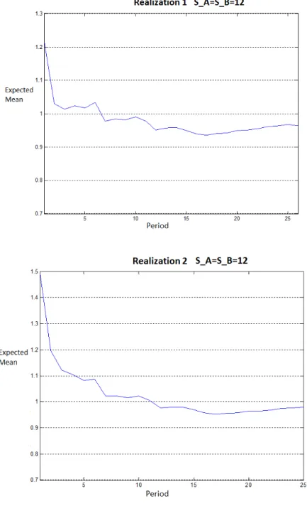
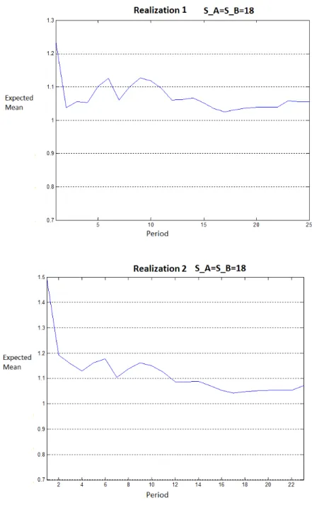
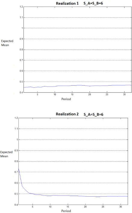
Estimation

In this section, we illustrate the convergence of the mean of the posterior dis-tribution to the assumed true mean and the speed of convergence. In all of our numerical examples, the customer arrivals are generated from a Poisson process with arrival rate of one per hour (λ = 1) and a period is taken to consist of 24 hours (τ = 24). It is assumed that stocks are replenished the beginning of each period to their prescribed maximum levels.

To illustrate the estimation of the arrival rate Λ, with known product prefer-ence and substitution rates, we considered the following setting with simulated samples. Then, the impacts of four different factors on the computed mean value of Λ is evaluated separately.

6.1.1

Priority Sensitivity

In this section, we examined the impact of prior distribution selection on the mean of the posterior density. For this approach, different mixing densities and weights are chosen for the prior mixture of gamma distributions. The impact on the posterior mean is evaluated in terms of cumulative mean absolute deviation (CMAD ). CMAD is sum of the absolute difference between estimated mean and actual mean over all periods. (CM AD =P

i(λi− λ)/n)

In this setting, we took the following set of parameters to generate the simula-tion data: r = (a, b, α, β) = (0.5; 0.5; 0.3; 0.3). Initial stock levels of both products A and B at the beginning of each period are taken as 12 (SA = SB = 12). We

have chosen five different η0, θ0 combinations for the prior mixture of gamma

densities. Then, for each η0, θ0 combination, 9 different values of mixture weight

c0 = (c01; c02) has been evaluated. Five different realizations are generated for

each η0, θ0, c0 combination. As it can be seen on Table 6.1, different expected