Land cover classification with multi-sensor fusion of partly missing data

(1)

Abstract

We describe a system that uses decision tree-based tools for seamless acquisition of knowledge for classification of remotely sensed imagery. We concentrate on three impor-tant problems in this process: information fusion, model understandability, and handling of missing data. Impor-tance of multi-sensor information fusion and the use of decision tree classifiers for such problems have been well-studied in the literature. However, these studies have been limited to the cases where all data sources have a full coverage for the scene under consideration. Our contribu-tion in this paper is to show how decision tree classifiers can be learned with alternative (surrogate) decision nodes and result in models that are capable of dealing with missing data during both training and classification to handle cases where one or more measurements do not exist for some locations. We present detailed performance evaluation regarding the effectiveness of these classifiers for information fusion and feature selection, and study three different methods for handling missing data in comparative experiments. The results show that surrogate decisions incorporated into decision tree classifiers provide powerful models for fusing information from different data layers while being robust to missing data.

Introduction

State-of-the-art remote sensing image analysis systems aid users by providing classification tools that use spectral information and possibly ancillary features as the input for statistical classifiers that are built using unsupervised or supervised algorithms. The tools that are based on maximum likelihood classification using parametric density models such as the Gaussian have the risk of failing to model the data adequately because complex features may not have such distributions. On the other hand, tools such as neural net-work classifiers or support vector machines that do not need any parametric density assumption require the user tune several magic parameters that are very much data dependent and are not always intuitive to select. Furthermore, most of these classifiers are used as black boxes that are evaluated by either visual inspection or statistical validation of the results

Land Cover Classification with Multi-Sensor

Fusion of Partly Missing Data

Selim Aksoy, Krzysztof Koperski, Carsten Tusk, and Giovanni Marchisio

using limited ground truth, and do not necessarily provide any means for understandability of the mapping from the input data to the output classification models.

Like any data analysis problem, domain knowledge and prior information are very useful in land-cover/land-use classification. Incorporating supplemental GISinformation and human expert knowledge into digital image processing has long been acknowledged as a necessity for improving remote sensing image analysis (Huang and Jensen, 1997). Artificial intelligence research and developments in rule-based classifi-cation systems have enabled a computer to mimic the heuris-tics and knowledge that a human expert uses in interpreting an image so that both computationally powerful and semanti-cally understandable classification models are developed.

Consequently, rule-based classification systems (Langley and Simon, 1995) have been successfully used in applications such as land-cover/land-use classification (Ton et al., 1991; Baraldi and Parmiggiani, 1994; Huang and Jensen, 1997; de Fries et al., 1998; Lawrence and Wright, 2001; Bardossy and Samaniego, 2002; Debeir et al., 2002), land-cover change monitoring (Wang, 1993; Rogan et al., 2003), aerial image interpretation (McKeown, Jr. et al., 1985), sea ice classification (Soh et al., 2004), tree classification for analyzing the effects of urbanization (Sugumaran et al., 2003), and ridge line extraction from Digital Elevation Model (DEM) data (Musavi et

al., 1999). These approaches used rule-based classification

with only spectral data (Ton et al., 1991; Bardossy and Samaniego, 2002; Sugumaran et al., 2003) as well as for information fusion from both spectral and ancillary data (Huang and Jensen, 1997; de Fries et al., 1998; Lawrence and Wright, 2001; Debeir et al., 2002; Rogan et al., 2003). Rule-based classifiers are particularly suitable for information fusion using different data modalities because conditions in rules correspond to ranges for numerical (continuous) data and set operations for categorical (discrete) data, and these conditions can be easily combined using Boolean operations.

However, a common problem in all of these attempts has been the translation of expert knowledge to a computer-usable format. Today, several commercial-of-the-shelf remote sensing image analysis systems have rule-based classification modules, but they operate on individual scenes and require an expert to create the rules. Even though rules constructed by experts may work well for particular cases (Ton et al., 1991; Wang, 1993; Soh et al., 2004), the requirement for an enormous amount of manual processing even for small data sets makes knowledge discovery in large remote sensing Selim Aksoy is with the Department of Computer

Engineering, Bilkent University, Ankara, 06800, Turkey ([email protected]).

Krzysztof Koperski and Carsten Tusk are with Evri, Inc., 206 1st_{Ave. South, Suite 310, Seattle, WA, 98104, and}

formerly with Insightful Corporation, Seattle, WA, 98109. Giovanni Marchisio is with Insightful Corporation, 1700 Westlake Ave. N., Suite 500, Seattle, WA, 98109.

Photogrammetric Engineering & Remote Sensing Vol. 75, No. 5, May 2009, pp. 577–593.

(2)

archives practically impossible. Furthermore, the use of these classifiers for information fusion has been limited to the cases where all data bands from all data sources are available for the scene under consideration, because the manually con-structed rules do not explicitly handle missing data in the measurements. The most popular alternative to the manual approach has been to use decision tree classifiers (Huang and Jensen, 1997; de Fries et al., 1998; Lawrence and Wright, 2001; Debeir et al., 2002; Rogan et al., 2003; Sugumaran et

al., 2003). However, portability and applicability of these

approaches to large and diverse data sets are still limited due to the manual involvement in the data preparation, rule creation, and final classification steps.

This paper describes our work on developing decision tree-based tools to automate the process of acquiring knowl-edge for analysis and classification of remotely sensed imagery. In this paper, we concentrate on three important problems in remote sensing image analysis: information fusion, model understandability, and handling of missing data. First of all, the non-parametric nature of decision tree classifiers that can operate on both numerical (continuous) and categorical (discrete) measurements without any assump-tions about neither the distribuassump-tions nor the independence of attribute values enables training of customized semantic land-cover/land-use labels from a fusion of visual and ancillary attributes. This is especially important for the fusion of measurements from different information sources. Secondly, a straightforward process of rendering the informa-tion in decision trees as logical expressions leads to decision rules for a knowledge base that consists of human readable classification models. Furthermore, the decision tree learning algorithms automatically perform feature selection by using only the attributes that can partition the measurement space the most effectively, and the resulting models are also often easy to interpret by creating subgroups of data which the user may graphically analyze. Finally, decision trees can be learned with alternative (surrogate) decision nodes, and this brings the capability of dealing with missing data during both training and classification to handle the cases where one or more measurements do not exist for some locations.

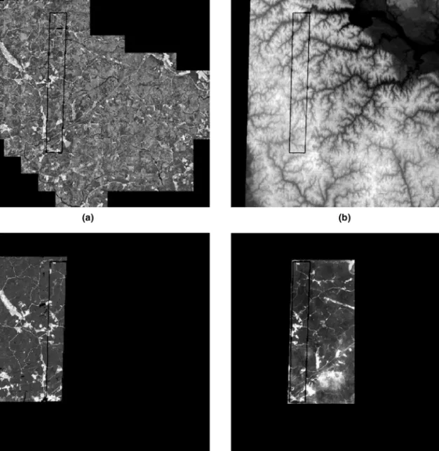
Decision tree classifiers and information fusion have both been extensively studied in the remote sensing literature. However, these studies have been limited to the cases where all data sources have a full coverage for the scene under consideration. On the other hand, presence of missing data is an important problem in statistical model-ing and analysis. There are several possible reasons for a value to be missing, such as: it was not measured; there was an instrument malfunction; the attribute does not apply; or the attribute’s value cannot be known. This is also an important problem in temporal and multi-sensor remote sensing image analysis where one or more data bands may be completely missing due to transmission problems, or there may be gaps in coverage of some of the sensors for particular regions at particular times (as can be seen in the coverage of our test data in Figure 1) because of satellite orbit restrictions, heavy clouds, haze or other atmospheric conditions, and viewing and illumination geometry.

Most algorithms “deal” with missing data by ignoring patterns with incomplete measurements (Little, 1978). Unless the relative amount of missing data is small, this is quite wasteful because remote sensing data are often hard and expensive to obtain. Furthermore, such discarding of patterns may also lead to valuable labeled data (ground truth) being thrown away, and may cause additional issues such as small sample size problems during training and adverse effects on the statistical significance of error rates during performance evaluation.

Our contribution in this paper is to show how decision tree classifiers can be learned with alternative (surrogate) decision nodes and result in models that are capable of dealing with missing data during both training and classifi-cation to handle cases where one or more measurements do not exist for some locations. We compare the perform-ance of the proposed classifiers to several other classifiers from the literature, and also evaluate the performance of three different methods for handling missing data. The rest of the paper is organized as follows. The multi-source data set that consists of spectral and textural values obtained from different aerial and satellite sensors with different coverages and resolutions is presented in the next section. The classifiers used for land-cover/land-use modeling are described followed by several methods for handling missing data. Performance evaluation using the multi-source data set is then presented followed by Conclusions.

Multi-source Data and Feature Extraction

The VISIMINEsystem (Koperski et al., 2002) we have developed supports interactive classification and retrieval of remote sensing images by modeling them on pixel, region, and scene levels. The system consists of a geospatial data

input/output library, a relational database management system, image processing, statistics, machine learning and data

mining libraries, and a graphical user interface. The inputs to the system are raw images and ancillary data. These data are automatically processed by unsupervised algorithms in the image processing library for feature extraction. Original data and extracted features become the input to the classification algorithms in the machine learning library. The user interacts with the system by providing a list of land-cover/land-use labels and corresponding training examples. The models learned from these examples can be used to classify other images in the same data set, or can be used to search other collections for similar scene structures.

The image data used in this paper consist of:

• Aerial (2 m/pixel ground resolution, three bands, one byte/pixel/band),

• Ikonos (4 m/pixel ground resolution, four bands, two bytes/pixel/band, two sets),

• DEM(30 m/pixel ground resolution, one band, two bytes/pixel/band)

data layers that cover the Fort A.P. Hill area in Virginia, USA, and were provided by the U.S. Army Topographic Engineer-ing Center. These layers were converted to the same projec-tion (WGS84, UTM Zone18) and were up-sampled (using nearest-neighbor interpolation of pixel values) to the same resolution (2 m) where each band has 11,683 ⫻ 11,677 pixels.

As additional ancillary data, we extracted Gabor wavelet features (Haley and Manjunath, 1999) for micro-texture analysis on several Aerial and Ikonos bands. Gabor features were computed by filtering a particular spectral band with Gabor wavelet kernels at different scales and orientations. We used kernels rotated by np/8, n⫽ 0, . . . ,7, at two scales. To obtain rotation invariant features, we computed the auto-correlation of the wavelet filter outputs with 0 and 90 degree phase differences at each scale. This resulted in four bands corresponding to two phase differences for each of the two scales. As a result, the extracted Gabor features correspond to:

• First band (red) of Aerial data (four texture bands, eight bytes/pixel/band),

• Second band (green) of Aerial data (four texture bands, eight bytes/pixel/band),

• First band of Ikonos data (four texture bands, eight bytes/pixel/band),

(3)

Figure 1. Data for the Fort A.P. Hill scene used in the experiments: (a) Aerial data (⬃391 sq. km. coverage), (b) DEMdata (⬃504 sq. km. coverage), (c) Ikonos2 data (⬃123 sq. km. coverage), and (d) Ikonos3 data (⬃101 sq. km. coverage). Note that each data layer has a different coverage of the same scene. The black pixels indicate missing data for that layer in that area. The black (red) polygon marks the common coverage area (⬃29 sq. km.). (The labels Ikonos2 and Ikonos3 in (c) and (d) are just the names of the corresponding data sets. These sets were obtained from the same sensor.) A color version of this figure is available at the ASPRSwebsite: www.asprs.org.

• Fourth band (near infrared) of Ikonos data (four texture bands, eight bytes/pixel/band).

The total size of the data (28 bands) is about 12 GB. Some of the data layers and their coverages are shown in Figure 1. The ground truth, which was also provided by the U.S. Army Topographic Engineering Center, includes 11 pixel level land-cover/land-use labels (classes) with independent training and testing data described in Table 1.

Decision Tree Classifiers and Information Fusion

This section describes the algorithms used in our decision tree classifier implementation and the details necessary for the description of the missing data handling methods.

Decision Tree Learning

Decision trees are non-parametric tools that are used to predict a categorical response (class) based on a collection of predictors (attributes, features). The fundamental principle underlying tree creation is that of simplicity. Each node in the tree includes a condition that splits (partitions) the data into groups. For a binary tree, the conditions are of the form “is x_{⑀ D” where x is a particular attribute and D is a subset} of the measurement space for that attribute. The cases for which the answer is “yes” belong to the branch representing set D, whereas the other cases go to the complement set -D. The preferred split condition makes the data reaching the immediate descendant nodes as “pure” as possible.

Decision trees can be built by recursively partitioning the training data where split functions are used to estimate

(4)

TABLE1. LAND-COVER/LAND-USECLASSES AND THENUMBER OFTRAINING ANDTESTINGEXAMPLES USED IN THEEXPERIMENTS. THESETRAINING ANDTESTINGEXAMPLES WEREGENERATED BYTWOPEOPLE USING THE GROUNDCONTROLPOINTS WITHIN THEORIGINALGROUNDTRUTHDATA. THEDIFFERENCES IN THENUMBER OF

EXAMPLES FOR DIFFERENTCLASSES ARECAUSED BY THESELABELINGS BYDIFFERENTPEOPLE AND DO NOT HAVE ANYSIGNIFICANTMEANINGRELATED TO THEDATA. THESENUMBERS AREPRESENTED ASTWO SEPARATECOLUMNS FOR THESUBSET THAT HASFULLCOVERAGE FORALLDATA SOURCES(SHOWN USING

THE“RED” POLYGON INFIGURE1) AND THEWHOLEDATA THATCONTAINMANYMISSINGPARTS. EACH CLASS ISREPRESENTED BY THECORRESPONDINGCOLOR IN THEFIGURES IN THEREST OF THEPAPER

Land-cover/ # training examples # testing examples

Land-use Color subset whole subset whole

burned 0 145 0 456 paved 188 91 80 536 building 17 664 93 427 ground 2,521 2,434 752 2,442 crop 0 9,433 0 49,765 grass 5,747 7,223 7,632 15,329 brush 1,565 3,117 2,292 7,170 pine 21,544 11,284 19,543 60,669 deciduous 10,942 10,409 4,936 59,511 water 9,130 14,275 8,194 41,502 marsh/wetland 2,233 7,204 3,589 8,097 Total 53,887 66,279 47,111 245,904

the impurities for partitioning. Let f be some impurity function and define the impurity of node A as:

(1) where pAiis the proportion of the training examples at node

A that belong to class i and m is the number of classes.

A requirement for f is that I(A) ⫽ 0 when A is pure and it achieves the largest value if all classes occur with equal frequency at that node. We use the entropy f(p) ⫽ ⫺p log(p) and the Gini f (p) ⫽ p(1 ⫺ p) functions for quantifying impurity (Therneau and Atkinson, 1999). The best split is defined to be the one that gives the maximal impurity reduction:

(2) where ALand ARare the left and right children of node

A and P(_{⭈) is the probability of a node. In Equation 2, the}

probability of node A can be computed as:

(3) where piis the prior probability for class i. Probabilities for

ALand ARare computed similarly. Given the training data, the partitioning algorithm searches through the attributes one by one and for each attribute finds the best split. Then, it compares the best single attribute splits and selects the best of the best. Next, the data are separated into two using that split, and this process is recursively applied to each subgroup until the subgroups either reach a minimum size or until no improvement can be made. Once the leaf nodes are found, they are labeled by the class that has the most patterns represented. The confidence value for that class is computed as the ratio of the training patterns that belong to that class to the total number of patterns in that node.

Tree-based tools have been considered as promising solutions for the information fusion problem in multi-source remote sensing with multi-sources such as spectral data,

DEMdata and other ancillary GIS data because they can operate on both numerical (continuous) and categorical

P(A)_{⫽ g}

m i⫽1

p_i p_Ai ¢I⫽ P(A)I(A) ⫺ P(A

L)I(AL)⫺ P(AR)I(AR)

I (A)⫽ g

m i⫽1

f (pAi)

(discrete) measurements. The split conditions on numeri-cal attributes are based on ranges of the measurement domain (e.g., “is x ⬍ x0”), whereas the conditions on

categorical attributes are based on subsets of the possible attribute values (e.g., “is x ⑀ { . . . }”). To decrease the computational load of the search procedure described above, we do randomized selection of candidate thresholds to find the split conditions for numerical attributes and consider randomized subsets of attribute values for categorical ones. Once the attributes are independently analyzed and the corresponding split conditions are found for each node of the decision tree, Boolean operations are used to combine these conditions and fuse the correspon-ding data modalities.

The resulting models are also often easy to interpret, even by those with no statistical expertise, by creating subgroups of data which the user may graphically analyze. Furthermore, they automatically perform feature selection during the searching phase of the splitting process using Gini or entropy selection criteria by using only the attributes that can partition the measurement space the most effectively. In particular, we use the predictor importance criterion which is measured for each data band (attribute) as the total reduction in the split criterion achieved by that band (attribute). An important attribute is defined as the one that maximizes the reduction in impurity given in Equation 2 as much as possible for as many nodes as possible. Therefore, given the impurity reduction values in Equation 2 for the attributes selected for each node in the tree, the overall importance value for a particular attribute is computed by summing the corresponding values in all nodes. The actual values of this criterion are not so important, but the relative sizes give an indication of the comparative utility of each attribute (Therneau and Atkinson, 1999).

Finally, depending on the threshold on the number of patterns at leaf nodes, the resulting tree can become a very extensive one that will actually classify the training samples perfectly but may have little generalization ability in classifying new observations (overfitting problem). To prevent such behavior and achieve good generalization ability, we use automatic pruning of trees based on error predictions and cost-complexity measures. In pruning, a tree with good classification accuracy on training data is fully

(5)

grown until leaf nodes have minimum size and minimum impurity. Then, the leaf nodes are successively deleted until a smaller tree with similar accuracy is obtained. We use cross-correlation to estimate the classification error during pruning. Trees can also be pruned using the cost complexity measure:

C(T,a)=R(T )+a`T` (4)

where T represents a tree, R(T) is the misclassification cost of T, and `T` is the number of leaf nodes in T. a acts as a penalty factor for the complexity of the tree. This cost-complexity measure C can be used to create a nested sequence of trees ordered according to their C values and cross-validation can be used to select the best tree from this sequence. Classifier ensembles that use bootstrap aggregation (bagging) with multiple feature subsets (Debeir et al., 2002), also called as random forests (Breiman, 2001), can alterna-tively be used for improving accuracy and generalization ability but we use single decision trees in this work to maintain straightforward interpretability of the classification models by the users.

Conversion of Trees into Rules

At any time of the learning process, decision trees can be automatically converted to decision rules. This can be done by tracing the tree from the root node to each leaf node and forming logical expressions that make the initial set of rules. Occasionally, some of these rules can be redundant and can be simplified without affecting the classification accuracy. We investigate the following schemes for rule generalization:

• Lossless generalization where conditions that are com-pletely redundant with respect to other conditions are removed. Redundancy is determined according to the intersection of decision regions, and complete redundancy occurs when a decision region for a particular attribute is covered by another decision region for the same attribute in the same rule.

• Lossy generalization where conditions are removed using greedy elimination. This is done by comparing error estimates of the original rule and the resulting rule with one of the conditions deleted. If the error rate for the latter case is no higher than that of the original rule, that condition is deleted. We use the pessimistic error estimate (Quinlan, 1993) where, given a confidence level, the upper limit on the probability of error is computed using the confidence limits for the Binomial distribution.

We also further simplify the rules by deleting the ones that have error estimates that are greater than the error estimate for the default rule. The default rule is used to assign the observations that do not satisfy any rule to the class with the highest frequency in the training data.

Examples of rule generalization are given below. Among the features used to construct these rules, FINE0DEG and COARSE0DEG are Gabor features computed from AERIAL data, ELEVATION is obtained from DEMdata, and the

integers given in curly brackets are the cluster IDs obtained by unsupervised clustering of the AERIAL data.

Example 1

(*) represents conditions removed based on error estimate, (**) represents conditions redundant with regard to ELEVATION _{⬍ 5.5.} non-generalized rule: IF AERIAL_GABOR::FINE0DEG ⬎⫽ 66.3421 (*) AND AERIAL_GABOR::COARSE0DEG ⬍ 253.842 (*) AND AERIAL::BAND1 ⬍ 142.5 (*) AND AERIAL::BAND2 ⬍ 76.5 (*) AND DEM::ELEVATION ⬍ 50.5 (**) AND DEM::ELEVATION ⬍ 10 (**) AND DEM::ELEVATION ⬍ 5.5 THEN CLASS water WITH PROB 1

generalized rule:

IF DEM::ELEVATION ⬍ 5.5

THEN CLASS water WITH PROB 0.99923 Example 2

(*) represents conditions removed based on error estimate, (**) represents conditions redundant with regard to ELEVATION ⬍ 35.5. non-generalized rule: IF AERIAL_GABOR::FINE0DEG ⬎⫽ 66.3421 (*) AND AERIAL_GABOR::COARSE0DEG ⬎⫽ 253.842 (*) AND AERIAL::CLUSTERID in {10–11,13,15–22} AND DEM::ELEVATION ⬍ 45.5 (**) AND AERIAL_GABOR::COARSE0DEG ⬍ 488.451 AND DEM::ELEVATION ⬍ 35.5 AND DEM::ELEVATION ⬎⫽ 32.5 THEN CLASS water WITH PROB 0.892006

generalized rule:

IF AERIAL::CLUSTERID in {10–11,13,15–22} AND AERIAL_GABOR::COARSE0DEG ⬍ 488.451 AND DEM::ELEVATION ⬍ 35.5

AND DEM::ELEVATION ⬎⫽ 32.5 THEN CLASS water WITH PROB 0.925682 Example 3

(*) represents conditions removed based on error estimate, (**) represents conditions redundant with regard to COARSE0DEG _{⬎⫽ 476.393.} non-generalized rule: IF AERIAL_GABOR::FINE0DEG ⬎⫽ 66.3421 (*) AND AERIAL_GABOR::COARSE0DEG ⬎⫽ 253.842 (**) AND AERIAL::CLUSTERID in {10–11,13,15–22} (*) AND DEM::ELEVATION ⬎⫽ 45.5 (*) AND AERIAL_GABOR::COARSE0DEG ⬎⫽ 476.393 AND DEM::ELEVATION ⬍ 60.5

THEN CLASS deciduous WITH PROB 0.666667

generalized rule:

IF AERIAL_GABOR::COARSE0DEG ⬎⫽ 476.393 AND DEM::ELEVATION ⬍ 60.5

THEN CLASS deciduous WITH PROB 0.85664

Decision trees always give sets of mutually exclusive rules. However, rules may not stay mutually exclusive after the rule generalization process (lossy generalization step). To avoid conflicts, we sort the rules in descending order of the probability (confidence) values. If an observation satisfies none of the rules, it is assigned to the default class that appears the most frequently in the training set.

Handling of Missing Data

Presence of missing data is an important problem in multi-temporal and multi-sensor remote sensing image analysis where one or more data bands may be completely missing due to transmission problems, or there may be gaps in coverage of some of the sensors for particular regions at particular times because of satellite orbit restrictions, heavy clouds, haze or other atmospheric conditions, and viewing and illumination geometry. However, most algorithms “deal” with missing data by ignoring patterns with incom-plete measurements and can work only on small scenes where complete data are available. This limits the use of multi-source data and hinders the exploitation of the complementary information inherent in such data.

Unless the relative amount of missing data is small, this is quite wasteful because remote sensing data are often hard

(6)

and expensive to obtain. Alternative techniques for handling missing data either impute all missing values before training or rely on the learning algorithm to deal with missing values in its training phase. These techniques are usually based on the assumption that the mechanism that results in the omission of a data point is independent of that point’s unobserved value. In particular, the data are assumed to be either missing at random (i.e., the distribution of which data points are missing depends on the complete data only through the observed data points) or missing completely at random (i.e., the distribution of which data points are missing does not depend on the observed or missing data) (Hastie et al., 2001).

A common technique for handling missing data is to make the calculations using only the attribute informa-tion present so that any pattern with at least one observed attribute will participate in training. When the learning algorithm involves estimation of parameters such as means and covariances, this corresponds to using only those observations for which measurements have been made on the relevant variables. Thus, the estimates for different attributes depend on different numbers of samples. How-ever, this can give poor results and may produce covari-ance matrices that are not positive definite (Webb, 2002). An alternative ad hoc solution is to replace a missing attribute by the mean or median of the non-missing values for that attribute, and treat it as if it was actually observed. A predictive model can also be estimated from the training patterns that are not missing a particular attribute, and a missing value can be imputed by its prediction from that model (Dixon, 1979; Little, 1978; Ghahramani and Jordan, 1994; Hastie et al., 2001). However, these imputations can bias and distort the marginal distributions of the attributes (Little, 1978). In addition, most of the existing solutions to the missing data problem assume that the training data are uncorrupted and missing values only in the test cases can be handled, thus potentially valuable data are neglected during training (Juszczak and Duin, 2004).

Classification models that can handle missing data during both training and application (test) phases have a high potential of making important contributions to remote sensing image analysis. We discuss three separate methods for handling missing data below. The first one is specific to decision tree classifiers whereas the other two can be used with any classifier.

Surrogate Splits

In our system, any observation with a class label and a value for at least one of the attributes participates in train-ing. To find the primary decision attribute and the corre-sponding split at a particular node, the criterion to be maximized is still Equation 2 where the first term is the same irrespective of missing data but the right two terms must be modified when there are incomplete observations (Therneau and Atkinson, 1999). For a particular attribute that is missing in some of the observations, first, the impu-rity values I(AL) and I(AR) and the probabilities P(AL) and

P(AR) are all computed over the observations that are not missing that attribute. Then, the probability values are adjusted so that they sum to P(A).

The procedure in the previous paragraph takes care of missing data during training. To be able to cope with missing data during the application of the classifier, the decision tree is extended using surrogate splits during training. The idea behind surrogate splits is to use the primary decision attribute at a node whenever possible, and use alternative attributes when the pattern is missing the primary attribute. This can be achieved by an ordered set of surrogate splits for each non-leaf node (Breiman et al., 1984; Duda et al., 2000).

Given the attribute that maximizes the impurity reduc-tion in Equareduc-tion 2 as the primary split at a node, the first surrogate split maximizes the probability of making the same decision as the primary split, i.e., the number of patterns that are sent to the same descendant branches by both the primary split and the surrogate split is as high as possible. Other surrogate splits are defined similarly and are ranked according to their misclassification errors. In addition to the surrogate splits, a blind rule called “go with the majority” is also evaluated. This rule chooses the descendant branch that received most of the training patterns. The surrogate splits that are stored for a particular node are the ones that do better than the blind rule in terms of classification accuracy. During the application phase, if a test pattern is missing the primary decision attribute at a node, it is classified using the first surrogate split, or if it is also missing that, the second surrogate is used, etc. If a pattern is missing all surrogate attributes, the blind rule is used, i.e., it is sent to the descendant node that received most of the training patterns (this is actually expected to be a very rare case).

Nearest Neighbor Imputation

As described above, imputation methods provide ad hoc solutions to the missing data problem. In our nearest neighbor imputation implementation, we take the subset of training data that contains only the patterns where all attributes are available (no missing data), and substitute the test data to create a full space of features where missing values are replaced by the corresponding values from the nearest neighbor of the test pattern in the training set. The nearest neighbor of a test pattern in the feature space is found according to the Euclidean distance between the corresponding feature vectors where only the non-missing features are used in the distance computation.

One-class Classifiers

An alternative method that can be applied to any classifier is to use a combination of one-class classifiers. The goal of one-class classification (Tax, 2001) is to accurately describe one class of patterns (called the target class) against the rest of the patterns (called outliers). Many standard pattern recognition techniques tackle this type of problem using two-class classifiers. Since these techniques require complete descriptions of both classes, they may not generalize well for the diverse (outlier) class. On the other hand, one-class classifiers try to overcome this problem by modeling only the target class and assuming a low uniform distribution for the outlier class.

After a probability density is estimated using the training patterns of the target class, a threshold is set on the tails of this distribution and a specified amount of the target data is rejected. This results in a decision boundary that separates the target class from the rest in the feature space.

One-class classifiers can be used to handle missing data as follows (Juszczak and Duin, 2004). First, individual one-class one-classifiers that use a single attribute at a time are trained. The resulting number of classifiers is dm where d is the number of attributes, and m is the number of classes. This keeps the number of required classifiers at a reasonable level as opposed to the alternatives such as training two-class two-classifiers on all possible combinations of attributes (resulting in classifiers) or training one-class one-classifiers on all possible combinations of attributes (resulting in (2d_{⫺ 1)m classifiers). Then, during testing, the} individual decisions by the classifiers corresponding to the available (non-missing) attributes are combined using Bayesian combination rules (Kittler et al., 1998). For these

(2d_{⫺ 1)}m(m⫺ 1) 2

(7)

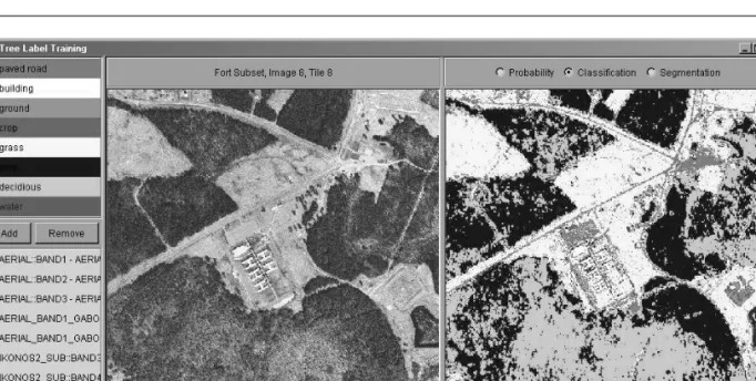
Figure 2. Graphical user interface for training classifiers. The panel on top-left shows the

land-cover/land-use classes defined by the user. The user can add new classes or remove existing ones, and can also change the color of a class. The panel on bottom-left shows the data layers used in training. The user can add or remove layers at any time of the training process, and examine the difference in classification results using the previously given training examples. Double-clicking on a data layer shows that layer on the left image panel. The “load tile” button loads a new image for training and/or classification. The “update” button shows the probability map for an individual class or the classification map for selected classes on the right image panel. The “undo” button removes the latest example submitted to the classifier. The “show info” button displays information about the trained classifier. The “show tree” and “show rules” buttons open the tree and rule displays,

respectively. A color version of this figure is available at the ASPRSwebsite: www.asprs.org. combinations, first, the posterior probabilities P(j ƒxi) are

estimated for classes j ⫽ 1, . . . ,m using individual

attributes xiwhere x⫽ (x1, x2, . . . , xd)Tis the full attribute vector. Then, as the final classification decision, a pattern x is assigned to class j* where:

(5)

using the product combination rule that simplifies the full posterior probability by assuming that the attributes are conditionally statistically independent, or:

(6)

using the sum combination rule that approximates the full posterior probability by assuming that the individual posterior probabilities do not deviate dramatically from the prior probabilities (Kittler et al., 1998). In both Equations 5 and 6, the product and sum are computed using only the available (non-missing) attributes.

Performance Evaluation

We evaluated the performance of the system using the Aerial, Ikonos, DEM, and Gabor data layers (consisting of a total of 28 bands in eight images) previously

j*_{⫽ arg max}m j⫽1 iH{availablea attributes} P(j

ƒ

x_i) j*_{⫽ arg max}m j⫽1 iH{availableq attributes} P(j

ƒ

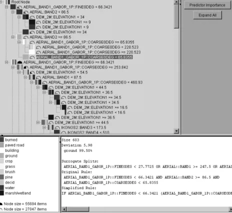
x_i)

described. Training of the classifiers is done using the graphical user interface shown in Figure 2 that allows users to add both training and testing (ground truth) examples. The user can view the color composite image or individual data bands while entering examples in the training display. At any time of the learning process, the user can view the current classification model as shown in Figure 3, and can validate it with the ground truth data using the automatically generated confusion matrices as shown in Table 3. In addition, the user can trace the results by selecting a rule (or an individual node in the tree) and see which patterns (pixels) are classified using that rule (or pass through that node during classification). Tracing also allows the user to select a pixel in the original image and see which rule and node are used to classify that pixel.

The experiments are grouped into four parts:

• evaluation of information fusion using decision tree classifiers,

• evaluation of rule generalization,

• evaluation of information fusion using other classifiers, and • evaluation of robustness to missing data.

Quantitative and qualitative results are presented below. Evaluation of Information Fusion using Decision Tree Classifiers The first set of experiments involved comparing the per-formance of combinations of different data layers using decision trees both for feature selection and as information

(8)

Figure 3. Graphical user interface for classification tree model visualization. Each node in the tree shows the primary split condi-tion and, for each class, percentages of training examples that satisfy that condition. Details of a node selected are also shown for further examination by the user. These details include the number of training examples (size) passing through that node, the Gini or entropy impurity value (deviation), surrogate splits, path from the root node to the current node (original rule), and the generalized rule if it is a leaf node. A color version of this figure is available at the ASPRSwebsite: www.asprs.org.

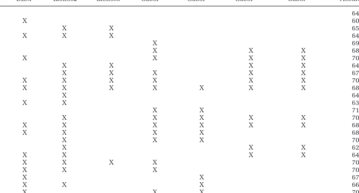
fusion tools. Table 2 presents 25 different combinations of data sources (images) and the corresponding correct classifi-cation rates using the ground truth. Pruning using the cost complexity measure given in Equation 4 was used during the learning of decision trees for each combination. The misclassification cost was estimated using ten-fold cross-validation and the complexity penalty a was set to 0.0001 empirically for pruning. Since the images used in the combinations contain a lot of missing data, surrogate splits were used as previously described. The Gini impurity function was used in the experiments reported. The result-ing differences when the entropy function was used were very insignificant in our data set.

The classification accuracy varied between 60 to 70 percent for the 25 combinations given in Table 2, with the maximum achieved as 71.16 percent when the three Aerial bands and the corresponding Gabor features were used. This is an expected result because the Aerial bands (and the corresponding Gabor features) have the largest coverage and do not need the approximations for handling of missing data. Another observation is that using Gabor features always improved the accuracy compared to the cases where no texture information was used. Among the optical bands, there was a slight increase in the accuracy when Ikonos bands were used together with Aerial bands. This shows that even though the Ikonos bands had a small coverage, the decision tree classifiers with surrogate splits could

incorpo-rate this information with the Aerial bands whenever possible. More detailed evaluation of information fusion and missing data handling are given in the following sections.

We also used decision trees for automatic feature selec-tion. In particular, the second set of experiments involved using the predictor importance criterion previously described to find the features (bands) that could partition the measure-ment space the most effectively. The advantage of this selection technique is that the importance values can be directly computed from the trained decision tree; therefore, no additional iterative search procedure is required for feature selection. The resulting importance values when all 28 features were given as input to the decision tree classifier are shown in Figure 4. The DEM(elevation) feature had the largest importance value. The reason behind this is that the

DEMdata originally have 30 m spatial resolution, but the version used in the classifier was up-sampled (interpolated) to 2 m for fusion with other data layers. Since the resulting neighboring pixels have the same value due to up-sampling,

DEMvalues seem to artificially have almost uniform values (low variance) for pixels belonging to the same class. This makes the importance value of DEMhigher than other bands even though this does not guarantee that DEMwill have good generalization ability for classification. Among the optical sources, the first two Aerial bands had the largest importance values. Given these two bands, the third (blue) band had a small significance. Ikonos bands had lower importance

(9)

TABLE2. COMBINATIONS OFDATASOURCES(IMAGES) AND THECORRESPONDINGCORRECTCLASSIFICATIONRATES WITHRESPECT TO THEGROUND TRUTH. ORIGINALDATASOURCES(AERIAL, DEM, IKONOS2, ANDIKONOS3) ARE SHOWN INFIGURE1. AERIALB1GABOR ANDAERIALB2GABOR

CORRESPOND TO THEGABORFEATURESEXTRACTED FROM THEFIRST AND THESECONDBANDS OF THEAERIALDATA, RESPECTIVELY. IKONOS2B1GABOR ANDIKONOS2B4GABORCORRESPOND TO THEGABORFEATURESEXTRACTED FROM THEFIRST AND THEFOURTH(NEAR-INFRARED)

BANDS OF THEIKONOS2 DATA, RESPECTIVELY. THECROSSMARK AT EACHCOLUMNMEANS THAT THEBANDS FROM THATIMAGE ARE USED IN THE COMBINATION IN THATROW. AERIALDATA WASASSUMED TO BEAVAILABLE INALLCOMBINATIONS BECAUSE IT HAS THEHIGHESTRESOLUTION

(THEMOSTDETAIL) AND THELARGESTCOVERAGE(EXCEPTDEM) AMONG ALLDATASOURCES

AerialB1 AerialB2 Ikonos2B1 Ikonos2B4

Aerial DEM Ikonos2 Ikonos3 Gabor Gabor Gabor Gabor Accuracy(%)

X 64.25 X X 60.82 X X X 65.68 X X X X 64.05 X X 69.57 X X X X 68.39 X X X X X 70.02 X X X X X 64.28 X X X X X X 67.99 X X X X X X X 70.50 X X X X X X X X 68.50 X X 64.22 X X X 63.71 X X X 71.16 X X X X X X 70.77 X X X X X X X 68.80 X X X X X 68.54 X X X X 70.87 X X X X 62.39 X X X X X 64.11 X X X X X 70.75 X X X X 70.67 X X X 67.08 X X X X 66.36 X X X X 70.20

Figure 4: Features sorted according to their predictor importance values. Out of 28 features, only the ones that constitute the cumulative 99 percent are shown. Details are given in the text.

values. This result is consistent with Table 2 where there was only a slight increase in the accuracy when Ikonos bands were used together with Aerial bands. Apart from the Aerial bands, Gabor features based on Aerial data constituted the next set of bands in the order of predictor importance. This result is also consistent with Table 2 and shows the impor-tance of texture features for land-cover/land-use classification. One final observation is that one does not have to use all

bands from the same source. The importance values for only a subset of such bands are high, and this shows the correla-tions among the bands and the importance of feature selec-tion within a problem that involves a lot of features. After the features were sorted according to their importance values and the ones that constitute the cumulative 99 percent importance were selected, the resulting subset of 15 features were given as input to the decision tree for classification. The overall accuracy was obtained as 70.92 percent (compared to 68.50 percent where all 28 bands were used). The confu-sion matrix for the resulting feature combination is given in Table 3. It can be seen that some classes (e.g., building, ground, pine, deciduous) had much higher accuracies compared to others (e.g., burned, paved, crop, brush, wet-land). This is due to the lack of qualified ground truth for some of the classes (e.g., burned areas, paved roads, and parking lots) and the spectral similarities that caused some confusion between certain pairs of classes (e.g., crop versus grass, grass versus brush, wetland versus water). Visual evaluation acknowledges correct classification of many classes including, e.g., roads and other paved areas in many cases.

Finally, the third set of experiments involved automatic feature selection using sequential forward selection and sequential backward selection algorithms (Duda et al., 2000). Sequential forward selection is an iterative algorithm that starts with a single feature and builds up a feature set by, at each iteration, adding the single best feature to the set of features selected in the previous iterations. The procedure starts with computing the classification accuracy when each feature is used individually, and selects the best one. Given this best one, pairs of features are formed using one of the remaining features and this best feature. The classification accuracy is computed for each pair, and the pair having the highest accuracy is selected. Given the best two features,

(10)

Figure 5. Results of sequential forward feature selec-tion: x-axis shows the classification accuracy (%), and y-axis shows the features added at each iteration (the first iteration is at the bottom). The highest accuracy value is shown with a star.

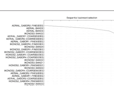
Figure 6. Results of sequential backward feature selection: x-axis shows the classification accuracy (%) and y-axis shows the features removed at each iteration (the first iteration is at the bottom). The highest accuracy value is shown with a star.

next, triplets of features are formed using one of the remain-ing features and these two best features. This procedure continues until all features are used.

Sequential backward selection is also an iterative algorithm that starts with all features and shrinks down the feature set by, at each iteration, removing the single worst feature from the set of features obtained in the previous iteration. The procedure starts with computing the classifica-tion accuracy when all d features are used. Then, the accuracies for all d-1 feature subsets are computed, and the subset having the highest accuracy is selected. This can also be interpreted as discarding the single worst feature. Next, the accuracies for all d-2 feature subsets of this best d-1 feature subset are computed, and the subset having the highest accuracy is selected. This procedure continues until one feature is left.

These procedures do not guarantee that the optimal subset of features is found but they allow us to select a suboptimal subset without doing an exhaustive search that would have required 228_{-1 classifications. Figures 5 and 6}

show the iterations of forward and backward selection, respectively. The best set of features obtained using sequen-tial forward selection contained 13 features with an overall accuracy of 72.12 percent. This subset consisted of three Aerial bands, seven Aerial-based Gabor features, two Ikonos bands, and one Ikonos-based Gabor feature as shown in Figure 5. The best set of features obtained using sequential backward selection contained eight features with an overall accuracy of 71.68 percent. This subset consisted of three Aerial bands, four Aerial-based Gabor bands, and one Ikonos band as shown in Figure 6. The results for individual classes were also consistent with those discussed above where most of the classes had similar accuracies as in the predictor importance criterion-based feature selection case, with the accuracies for some of the classes (e.g., building, ground, crop, wetland) improved even further. Note that these selection results were not affected by the artificial low variance of the DEMdata because they used the classification error directly as the search criterion. We can conclude that,

TABLE3. CONFUSIONMATRIX FOR THEDECISIONTREE CLASSIFIER USING THE15 FEATURESSELECTEDACCORDING TO THEIRPREDICTORIMPORTANCEVALUES

Assigned

Total %Agree

burned paved building ground crop grass brush pine deciduous water marsh

burned 24 0 0 0 0 0 0 172 23 187 50 456 5.26 paved 0 38 33 47 9 111 136 2 55 105 0 536 7.09 building 0 0 366 10 0 24 0 0 4 23 0 427 85.71 ground 0 1 4 2022 0 211 31 10 157 6 0 2442 82.80 crop 0 0 0 2976 18163 17740 7415 1899 488 559 525 49765 36.50 True grass 0 20 19 311 1053 10309 3339 9 252 10 7 15329 67.25 brush 0 0 0 209 464 2175 2514 61 1707 37 3 7170 35.06 pine 13 15 9 7 378 8 578 51767 1607 2507 3780 60669 85.33 deciduous 0 31 53 32 86 77 697 3044 53278 608 1605 59511 89.53 water 75 0 20 2 212 6 3 784 571 32119 7710 41502 77.39 marsh 119 21 2 0 12 0 1 1176 1166 1808 3792 8097 46.83 Total 231 126 506 5616 20377 30661 14714 58924 59308 37969 17472 245904 70.92

(11)

TABLE4. CONFUSION MATRIX FOR THERULE-BASEDCLASSIFIER USING THE13 FEATURESSELECTEDACCORDING TO THESEQUENTIAL FORWARDFEATURESELECTIONALGORITHM

Assigned

burned paved building ground crop grass brush pine deciduous water marsh

burned 0 0 0 0 0 0 0 310 34 99 13 456 0.00 paved 0 21 90 43 2 113 97 2 102 66 0 536 3.92 building 0 0 390 6 0 7 0 0 3 21 0 427 91.33 ground 0 0 2 2148 0 86 16 8 177 5 0 2442 87.96 crop 0 1 0 3174 22174 16551 3531 2291 1727 218 98 49765 44.56 True grass 0 6 21 201 182 11515 3068 10 303 22 1 15329 75.12 brush 0 0 0 163 423 1410 3099 31 2022 22 0 7170 43.22 pine 0 1 23 0 873 0 6 54411 1980 1165 2210 60669 89.69 deciduous 0 5 29 156 147 118 612 4112 52815 700 817 59511 88.75 water 0 0 12 1 306 0 0 1350 401 36091 3341 41502 86.96 marsh 0 2 12 0 14 0 1 1955 1072 2353 2688 8097 33.20 Total 0 36 579 5892 24121 29800 10430 64480 60636 40762 9168 245904 75.38

in overall, fusion of spectral and textural features as well as feature selection improved the classification accuracy. Evaluation of Rule Generalization

We also evaluated the effects of rule generalization on classification. Three experiments with different feature sets were performed. These experiments correspond to the fea-ture sets selected according to the predictor importance, sequential forward selection, and sequential backward selection algorithms. Decision trees were trained using these features, and the corresponding generalized rule sets were constructed from these trees as described. The overall classification accuracies obtained using the features based on predictor importance, forward selection and backward selection were 74.81 percent, 75.38 percent, and 75.10 percent, respectively. As an example, the confusion matrix for the 13-feature subset obtained using sequential forward selection is shown in Table 4. In all cases, the classification accuracy for the rule-based classifier consisting of the generalized rules learned from the decision tree classifier was higher than the one for the corresponding decision tree classifier. The improvement was due to the additional pruning during rule generalization.

Evaluation of Information Fusion using Other Classifiers

We compared the decision tree classifiers with the maxi-mum likelihood classifier, support vector machine classifier, minimum distance classifier, naive Bayes classifier, tree ensemble using boosting and tree ensemble using bagging available in the VISIMINEsystem. Our maximum likelihood classifier implementation uses Gaussian mixture models for class-conditional densities. Each component in the mixture has an arbitrary covariance matrix where the parameters of the model are estimated using the Expectation-Maximization algorithm (Duda et al., 2000). Our support vector machine (SVM) classifier implementation uses both linear and polyno-mial kernels for mappings from the original feature space to a high-dimensional space where the training examples for different classes can be separated by hyperplanes. SVM

classifiers are originally developed for binary classification and our implementation uses the decision-directed acyclic graph approach (Platt et al., 2000) for extension of SVMs to multi-class classification. The minimum distance classifier forms clusters of input training examples and labels a test pattern with the label of the cluster whose centroid is closest to the feature vector of that pattern (Duda et al., 2000). The naive Bayes classifier uses the Bayes decision

rule with the conditional independence assumption that states that features are independent given the class label for a pattern (Duda et al., 2000). Our implementation models class-conditional probabilities using Gaussian mixtures. Bagging uses multiple bootstrapped versions of the original training data where each of these bootstrap data sets is used to train a different component classifier and the final classification decision is based on the vote of each compo-nent classifier (Breiman, 1996). Boosting also iteratively generates new training sets where the probability of a data point being selected for a component classifier is determined according to how accurately it was classified by earlier component classifiers. The final classification decision is based on the weighted sum of the outputs of the component classifiers (Schapire, 2002).

Since these additional classifiers cannot handle missing data, we used the subset of the training data that includes the intersection of the coverages of all sensors (see Figure 1). We also used only the Aerial data and the Gabor features corresponding to the second (green) band because of compu-tational reasons for some of the classifiers. The resulting performances for different classifier settings are given in Table 5. As can be seen from the results, the performances for different classifiers were similar to each other except the minimum distance and the naive Bayes classifiers that could not perform as well as the others. An important observation is that the common accuracy, which was close to 90 percent, for this data set was greater than the accuracy values (⬃70 percent) obtained by the decision tree classifiers for the whole data. The main reason behind this is the presence of large amounts of missing data in the original data set. In addition, these results do not include the “burned” and “crop” classes as they were removed from the training data because no ground truth examples exist for these classes in the small coverage area. Some of the increase in classification accuracy can be attributed to this removal because these two classes cannot be classified accurately as can be seen from the confusion matrices discussed earlier. Finally, the remaining ⬃10 percent error for the fully available data set can be associated with the complexity of the land-cover/land-use classes in the high-resolution imagery and the spectral similarities among these classes.

We also used hypothesis testing to further evaluate the significance of the differences between the performances of different classifiers. The McNemar test (Dietterich, 1998; Debeir et al., 2002) is used to check whether the predictions

(12)

TABLE5. PERFORMANCE OFDIFFERENTCLASSIFIERS FOR ASUBSET OF THEORIGINALDATA WHERE THERE ISCOMPLETE COVERAGE(SHOWN USING THE“RED” POLYGON INFIGURE1). THENOTESCOLUMNDESCRIBES THESETTINGS OF

APARTICULARCLASSIFIER

Classifier Notes Accuracy(%)

Decision tree (DT-CC) Pruned using the cost-complexity measure 87.85 Decision tree (DT-CV) Pruned using cross-validation 88.20 Maximum likelihood (ML-1) Single multivariate Gaussian for each class 86.28 Maximum likelihood (ML-2) Mixture of 2 Gaussians for each class 87.83 Maximum likelihood (ML-3) Mixture of 3 Gaussians for each class 89.22 Maximum likelihood (ML-4) Mixture of 4 Gaussians for each class 88.87

Support vector machine (SVM-L) Linear kernel 87.97

Support vector machine (SVM-P) Polynomial kernel 90.20

Minimum distance (MD) 66.78

Naive Bayes (NB) 72.97

Boosted tree ensemble (BS-30) 30 components 89.01

Boosted tree ensemble (BS-35) 50 components 89.09

Bagged tree ensemble (BG-30) 30 components 88.34

Combined classifiers (COMB) Tree ⫹ SVM ⫹ Maximum likelihood 90.24

TABLE6. MCNEMARTESTRESULTS. THENUMBERSSHOW THE P-VALUES FOR THECORRESPONDINGPAIR OFCLASSIFIERS. A P-VALUE BEINGGREATER THAN THESIGNIFICANCELEVELa_{⫽ 0.05 (S}HOWN ASBOLD) MEANS THAT THERE IS NOSIGNIFICANT

DIFFERENCE BETWEEN THEPREDICTIONS OF THECORRESPONDINGCLASSIFIERS. CLASSIFIERNAMES ARE GIVEN INTABLE5

DT-CC DT-CV ML-1 ML-2 SVM-P BS-30 BG-30 COMB DT-CC — 0.5071 0.0000 0.0000 0.0000 0.0000 0.0000 0.0000 DT-CV — 0.0000 0.0000 0.0000 0.0000 0.0000 0.0000 ML-1 — 0.0000 0.0000 0.0000 0.0000 0.0000 ML-2 — 0.0000 0.0000 0.0000 0.0000 SVM-P — 0.0000 0.0000 0.0000 BS-30 — 0.3057 0.0030 BG-30 — 0.0350 COMB —

of two classifiers trained with the same training data differ significantly among themselves. Given two classification algorithms A and B, we count the number of data points misclassified by A but not by B (denoted n01), and the

number of examples misclassified by B but not by A (denoted n10). Under the null hypothesis, there is no

difference between the classifiers’ predictions and they have the same error rate, which means that n01⫽ n10.

The test statistic:

(7) follows a x2_{distribution with one degree of freedom under}

this hypothesis. Given a significance level a, we can find the rejection region where the probability that the test statistic T is greater than a critical value is less than a. For example, for

a⫽ 0.05, this critical value is found as x2

1,0.95⫽ 3.8415.

If the test statistic is greater than this value, we can reject the null hypothesis in favor of the hypothesis that the difference between the performances of two classifiers is significant. The significance of this difference for different classifier pairs can be quantified by the p-value which is the probability of making a Type I error that occurs when the null hypothesis is true (i.e., there is no difference between the two classifiers) and the test rejects the null hypothesis.

The McNemar test was performed to evaluate the significance of the difference between the performances of different classifiers. Among the 28 different pairs of classi-fiers compared, only two cases had a p-value greater than the significance level (i.e., there was no significant difference) as shown in Table 6. These cases were: decision trees pruned

T⫽(

ƒ

n₀₁⫺ n₁₀

ƒ

⫺ 1)2

n₀₁_{⫹ n}₁₀

using the cost-complexity measure vs. cross-validation, and classifier ensembles formed using boosting versus bagging. These two cases were expected because the classifiers compared were based on similar structures and were trained using similar algorithms. All other pairs were found to be significantly different.

These comparative experiments show that the decision tree classifiers perform at least as good as many other classifiers (even their combinations) on the data with full coverage. Therefore, decision trees can be considered useful and effective tools for information fusion with the additional important advantage that they can handle missing data without a significant decrease in performance. On the other hand, many commonly used classifiers can only classify a small subset of the original data where there is complete coverage. In other words, for our data set, they can perform information fusion only for ⬃6 percent of the original data (in terms of area with respect to the data source with the largest coverage) as shown in Figure 1 and Table 1. Evaluation of Robustness to Missing Data

We evaluated the robustness of decision tree classifiers to missing data using three methods:

• using surrogate splits,

• using nearest neighbor imputation, and • using combinations of one-class classifiers.

The Aerial data, the Ikonos data, the Gabor features extracted from the first and the second bands of the Aerial data, and the Gabor features extracted from the first and the fourth bands of the Ikonos data (total of 23 bands) were used as features.

(13)

TABLE7. CONFUSIONMATRIX FOR THEDECISIONTREECLASSIFIER USINGSURROGATESPLITS FORHANDLINGMISSINGDATA

Assigned

paved building ground grass brush pine deciduous water marsh

paved 270 1 12 43 50 23 134 3 0 536 50.37 building 22 240 7 30 3 10 114 1 0 427 56.21 ground 6 0 2183 35 11 5 194 5 3 2442 89.39 grass 13 0 183 11450 1738 93 1835 17 0 15329 74.70 True brush 3 0 205 1787 3230 151 1772 21 1 7170 45.05 pine 0 0 0 0 13 56076 902 1115 2563 60669 92.43 deciduous 1 0 85 63 764 5674 52637 40 247 59511 88.45 water 0 0 0 0 4 2827 214 34599 3858 41502 83.37 marsh 0 0 0 0 0 1960 78 1579 4480 8097 55.33 Total 315 241 2675 13408 5813 66819 57880 37380 11152 195683 84.40

For all three methods, the subset of data where there is complete coverage (no missing parts) was used for training so that the classification models were learned from patterns that have values for all features. Same as in the previous section where different classifiers were compared, the “burned” and “crop” classes were removed because no training ground truth examples exists for these classes in the area where there is complete coverage of all features. To test the classifiers, full test data (see Table 1) were used.

The confusion matrices for surrogate splits, nearest neighbor imputation, and combinations of one-class classi-fiers are given in Tables 7, 8, and 9, respectively. The highest accuracy was obtained as 84.40 percent when

surrogate splits were used for handling missing data. On the same data set, nearest neighbor imputation and one-class classifiers achieved 84.19 percent and 47.08 percent accura-cies, respectively. Even though combinations of one-class classifiers can be applied to any classifier as previously described, their performance was significantly lower than those of other missing data handling techniques on this data set. One possible reason for this may be the use of each feature independently for the classifiers used in the combi-nation. We believe that independent usage of the features could not model the complex data and the complex set of classes in this problem setting. Another justification for this observation can be found in the relatively low performance

TABLE8. CONFUSIONMATRIX FOR THEDECISIONTREECLASSIFIER USINGNEARESTNEIGHBORIMPUTATION FORHANDLINGMISSINGDATA

Assigned

TABLE9. CONFUSIONMATRIX FOR THEDECISIONTREECLASSIFIER USINGCOMBINATIONS OFONE-CLASSCLASSIFIERS FORHANDLINGMISSINGDATA

Assigned

(14)

of the naive Bayes classifier that uses the same independ-ence assumption in the experiments presented in the previous section.

The nearest neighbor imputation technique achieved similar performance as the surrogate splits technique. However, the classifier resulting from the use of surrogate splits has the additional advantage of providing a classifi-cation model with higher understandability and inter-pretability due to the direct incorporation of the surrogate (alternative) conditions into the decision rules (see Figure 3 for an example). Furthermore, the surrogate splits-based classifier has faster run-time performance because of the additional cost of computing distances in the nearest neighbor imputation technique.

When these results in Table 7 are compared to those in Tables 3 and 4 with accuracies around 70 to 75 percent, we can see an improvement of around 10 percent. The reason for this improvement is that the subset of data where there is complete coverage was used for training in the former case (Table 7) but the whole training data, with many missing areas, were used in the latter case (Tables 3 and 4). There-fore, the learned classification models were more accurate in the sense that they were learned from data where all features for all patterns were available. (The same testing data were used for all of these cases (Tables 3, 4, and 7).) When the results of Table 7 are compared to those in Table 5, the improvement of around 4 percent in the latter case can be attributed to the use of testing data where all features for all patterns were available. (The same training data where used for all of these cases (Tables 5 and 7).)

Evaluation Summary

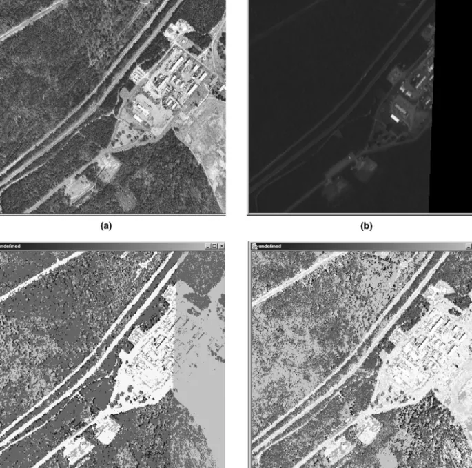
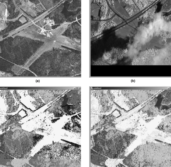
The conclusions of the experiments in the Performance Evaluation Section can be summarized as follows. When there were missing data in the training set, using only the subset where there was complete coverage (no missing parts) gave better results (Table 7 versus 3 and 4). When there was missing data in the testing set, the accuracy using only the subset where there was complete coverage (Table 5) was higher than the accuracy for the whole data where some features were missing for some patterns (Tables 3, 4, and 7), but using surrogate splits allowed classifying the whole data (⬃17 times more area than the subset) without a significant difference (⬃4 percent) in the overall accuracy. As visual examples, Figures 7 and 8 illustrate classification in the presence of missing data. Aerial and Ikonos bands were used in these examples. Missing data in the Ikonos bands initially resulted in many false alarms. However, land-cover/land-use classification drastically improved when surrogate splits were used.

Conclusions

We described decision tree and rule-based tools for building statistical land-cover/land-use models for classification of remote sensing images. We concentrated on three important problems in the image analysis process: information fusion, model understandability, and handling of missing data.

We presented detailed performance evaluation of the proposed models and algorithms using a very large multi-source data set consisting of spectral, textural and DEM

data layers with a total of 28 data bands. An extensive set of experiments consisting of comparisons of 25 different combinations of data sources illustrated that decision tree clas-sifiers are capable of fusing information from different sources and handling missing observations in these sources. These experiments also proved that the proposed classifiers can be used for feature selection in parallel to building classifica-tion models. In the next set of experiments, the rule-based

classifier consisting of the generalized rules learned from a decision tree classifier had a higher accuracy than the corre-sponding tree classifier due to the additional pruning during rule generalization. We also performed comparative experi-ments using six other popular classification techniques and showed that the decision tree classifiers perform at least as good as many other classifiers (even their combinations) with the additional important advantage of providing classification models with higher understandability and human readability. Furthermore, evaluation of the robustness of these classifiers to missing data illustrated that surrogate splits incorporated into decision trees and rules can robustly handle missing data with a higher accuracy than two other comparative techniques.

Overall, the decision tree classifiers and the correspon-ding rules proved to be very powerful and flexible in building land-cover/land-use models by fusing information from different data layers while being very robust to missing data during both training and classification. Our current work includes developing new methods for region segmentation, and building human readable models that are learned for characterizing the contents of the resulting image objects using shape attributes and statistical sum-maries of their spectral and textural features.

Acknowledgments

This work was supported by the U.S. Army contracts DACA42-03-C-16 and W9132V-04-C-0001. S. Aksoy was supported in part by the TUBITAK CAREER Grant 104E074 and European Commission Sixth Framework Programme Marie Curie International Reintegration Grant MIRG-CT-2005-017504. The VISIMINEproject was also supported by NASA contracts NAS5-98053 and NAS5-01123.

References

Baraldi, A., and F. Parmiggiani, 1994. A Nagao-Matsuyama approach to high-resolution satellite image classification,

IEEE Transactions on Geoscience and Remote Sensing,

32(4):749–758.

Bardossy, A., and L. Samaniego, 2002. Fuzzy rule-based classifica-tion of remotely sensed imagery, IEEE Transacclassifica-tions on

Geoscience and Remote Sensing, 40(2):362–374.

Breiman, L., 1996. Bagging predictors, Machine Learning, 24(2):123–140.

Breiman, L., 2001. Random forests, Machine Learning, 45(1):5–32. Breiman, L., J.H. Friedman, R.A. Olshen, and C.J. Stone, 1984.

Classification and Regression Trees, Wadsworth and

Brooks/Cole.

de Fries, R.S., M. Hansen, J.R.G. Townshend, and R. Sohlberg, 1998. Global land cover classifications at 8km spatial resolution: The use of training data derived from Landsat imagery in decision tree classifiers, International Journal of Remote

Sensing, 19(16):3141–3168.

Debeir, O., I.V. den Steen, P. Latinne, P.V. Ham, and E. Wolff, 2002. Textural and contextual land-cover classification using single and multiple classifier systems, Photogrammetric Engineering &

Remote Sensing, 68(6):597–605.

Dietterich, T.G., 1998. Approximate statistical tests for comparing supervised learning algorithms, Neural Computation, 10(7):1895–1923.

Dixon, J.K., 1979. Pattern recognition with partly missing data,

IEEE Transactions on Systems, Man, and Cybernetics,

9(10):617–621.

Duda, R.O., P.E. Hart, and D.G. Stork, 2000. Pattern Classification, John Wiley & Sons, Inc.

Ghahramani, Z., and M.I. Jordan, 1994. Supervised learning from incomplete data via an EM approach, Advances in Neural

(15)

Figure 7. Classification in the presence of missing data: (a) Aerial bands, (b) Ikonos band with missing data, (c) Classification using no surrogate splits, and (d) Classification using five surrogate splits. Missing data in the Ikonos bands (see Figure 1c and 1d) resulted in false results for the right half of the scene. However, recognition of buildings as well as land-cover/land-use classification drastically improved when surrogate splits were used. A color version of this figure is available at the ASPRSwebsite: www.asprs.org.

Haley, G.M., and B.S. Manjunath, 1999. Rotation-invariant texture classification using a complete space-frequency model,

IEEE Transactions on Image Processing, 8(2):255–269.

Hastie, T., R. Tibshirani, and J. Friedman, 2001. The Elements of

Statistical Learning, Springer Series in Statistics.

Huang, X., and J.R. Jensen, 1997. A machine-learning approach to automated knowledge-base building for remote sensing image analysis with GIS data, Photogrammetric Engineering & Remote

Sensing, 63(10):1185–1194.

Juszczak, P., and R.P.W. Duin, 2004. Combining one-class classifiers to classify missing data, Proceedings of the 5th_{International}

Workshop on Multiple Classifier Systems, pp. 92–101.

Kittler, J., M. Hatef, R.P.W. Duin, and J. Matas, 1998. On combining classifiers, IEEE Transactions on Pattern Analysis and Machine

Intelligence, 20(3):226–239.

Koperski, K., G. Marchisio, S. Aksoy, and C. Tusk, 2002. VisiMine: Interactive mining in image databases, Proceedings of IEEE

International Geoscience and Remote Sensing Symposium,

Toronto, Canada, Vol. 3, pp. 1810–1812.

Langley, P., and H.A. Simon, 1995. Applications of machine learning and rule induction, Communications of the ACM, 38:55–64. Lawrence, R.L., and A. Wright, 2001. Rule-based classification systems

using classification and regression tree (CART) analysis,

Pho-togrammetric Engineering & Remote Sensing, 67(10):1137–1142.

Little, R.J.A., 1978. Consistent regression methods for discriminant analysis with incomplete data, Journal of the American

Statistical Association,73:319–322.

McKeown, Jr., D.M., W.A. Harvey, Jr., and J. McDermott, 1985. Rule-based interpretation of aerial imagery, IEEE Transactions