KiMPA: A Kinematics-Based Method for
Polygon Approximation
Ediz S¸aykol, G¨urcan G¨ule¸sir, U˘gur G¨ud¨ukbay and ¨Ozg¨ur Ulusoy
Department of Computer Engineering, Bilkent University 06533 Bilkent, Ankara, Turkey
{ediz,gulesir,gudukbay,oulusoy}@cs.bilkent.edu.tr
Abstract. In different types of information systems, such as multimedia information systems and geographic information systems, object-based information is represented via polygons corresponding to the boundaries of object regions. In many applications, the polygons have large number of vertices and edges, thus a way of representing the polygons with less number of vertices and edges is developed. This approach, called poly-gon approximation, or polypoly-gon simplification, is basically motivated with the difficulties faced in processing polygons with large number of vertices. Besides, large memory usage and disk requirements, and the possibility of having relatively more noise can also be considered as the reasons for polygon simplification. In this paper, a kinematics-based method for polygon approximation is proposed. The vertices of polygons are sim-plified according to the velocities and accelerations of the vertices with respect to the centroid of the polygon. Another property of the proposed method is that the user may set the number of vertices to be in the approximated polygon, and may hierarchically simplify the output. The approximation method is demonstrated through the experiments based on a set of polygonal objects.
1 Introduction
In most of the information systems employing methods for representing or retrieval of object-based information, polygons are used to represent objects or object regions, corresponding to the boundaries of the ob-ject regions. For example, in multimedia information systems, polygons are used in pattern recognition, object-based similarity [1, 14], and image processing [12]. Another example application can be the representation of geographic information by the help of polygons in geographic infor-mation systems [6]. In many cases, the polygons have large number of vertices, and managing these polygons is not an easy task. Thus, polygon approximation is required to facilitate information processing. Obviously, the output of the approximation must be a polygon preserving all of the critical shape information in the original polygon. Besides the difficul-ties in managing polygons with large number of vertices, storing such a
polygon may require relatively large disk space and memory usage during processing. However, the simplified form requires less memory and disk space than the original one. Another reason for using polygon approxi-mation can be the fact that the simplified form of the original polygon tends to have less ‘noise’ as far as the small details on the object region boundaries are concerned.
In [13], a tool for object extraction in video frames, called Object Ex-tractor, is presented in which the boundaries of the extracted object re-gions are represented as polygons. Basically, the extracted polygons have at least 360 vertices for each angle with respect to the centroid of the object. Since such a size is quite large as we might have a large number of objects in a single video frame, an approximation for the polygons is inevitable. Since dealing with polygons having appropriate size is one of the main motivations of polygon approximation, a reasonable size for the approximated polygons is around 30 vertices. For example, Turning An-gle Method [1], a famous polygonal shape comparison method, may not be feasible for polygons having more than 30 vertices. In this method, a (polygonal) object is represented by a set of vertices and shape compar-ison between any two objects is performed with respect to their turning angle representations. A turning angle representation of an object is the list of turning angles corresponding to each vertex on the polygon.
In this paper, Kinematics-Based Method for Polygon Approximation (KiMPA) is proposed. The main motivation of using kinematics is to figure out the most ‘important’ vertices to appear in the approximated form via associating a level of importance for each of the vertices. Thus, KiMPA eliminates less important vertices until the polygon reduces to an appropriate size. The rest of the paper is organized as follows: Sec-tion 2 defines the polygon approximaSec-tion problem formally and discusses some of the existing methods in the literature. The KiMPA approxima-tion process is discussed in Secapproxima-tion 3. In Secapproxima-tion 4, the experiments to demonstrate approximation method are presented for a set of polygonal objects. Finally, Section 5 concludes the paper.
2 Related Work
In parallel to the wide use of polygons in information systems, polygon approximation methods are required in various application areas, such as pattern recognition [10], processing spatial information [6], and shape cod-ing [8]. Besides, there are also methods applicable to many applications.
Before discussing some of the existing polygon approximation methods, the problem definition is given first.
2.1 Problem Definition
The problem of polygon approximation can be defined as follows: Let a set of points P = {p1, p2, ..., p|P |} denote a polygon (|P | is possibly
large). Let another set of points PA = {p1, p2, ..., p|PA|} denote another
polygon. If |P | >> |PA| and dP,PA < ², where dP,PA denotes the difference
between P and PA, and ² denotes the approximation error, then PAis an
approximation of P . Based on this definition, the polygon approximation problem can be classified into two as follows:
– Given an upper bound for ², find the polygon with minimum number of vertices.
– Given an upper bound for |PA|, find the polygon that minimizes the
approximation error ².
In many applications, the main goal may not fit into the above cases. For example in [13], due to the complexity of the extracted object bound-ary polygons, the approximated polygon must have less number of sides than some threshold (|PA|) and the approximation error must be below
some threshold (²). However, the approximated polygon must preserve the critical shape information, thus must include the most important vertices. The most important vertices are the peaks, i.e., the sharp and extreme points. Therefore, the approximation algorithm has to eliminate the non-critical vertices first.
2.2 Polygon Approximation Methods
The first way of approaching polygon approximation problem can be se-lecting |PA| many vertices from P arbitrarily or at random. In many cases,
this may not give the desired results. Thus, more sophisticated methods are needed for an appropriate approximation.
There exist some methods that transform the polygon approximation to a graph-based problem [4]. The corresponding weighted graph G for a polygon P is constructed as follows: Each vertex of the polygon is set to be a node in G, and arcs are added for each vertex pair (i, j) such that i < j. An error is associated for each arc corresponding to the presence of the line segment pipj in the approximated form. Due to this transformation,
solving the shortest path problem in G is equivalent to the first group of polygon approximation problems, as mentioned in problem definition.
The Minimax Method [9], however, finds an approximation for a set of points representing a polygon where for an approximated line l the maximum distance between the points and l is minimized. The method is generalized for polygonal curves, not only closed polygons, and different constraints are imposed according to the definition and specifications of the problem. Another method that minimizes the inflections is proposed by Hobby [7]. In this method a special data structure is designed for the set of points so that the direction and length of the approximating line between points can be determined. The main use of such a method may be approximating the scanned bitmap images to smooth polygons.
Polygon simplification algorithms in computer graphics literature re-duce the number of polygons in a three dimensional polygonal model containing a large number of polygons [5, 11, 15]. However, since our aim is simplifying a two dimensional polygon by reducing the number of ver-tices and edges, we seek a more specialized algorithm suitable for this purpose. Although more general polygonal simplification algorithms from computer graphics domain can be used with adaptations for our specific needs, we preferred to design a new algorithm since the polygonal simpli-fication algorithms from graphics domain are more general, and therefore, more complicated. However, our algorithm is similar to polygon simplifi-cation algorithms using vertex decimation.
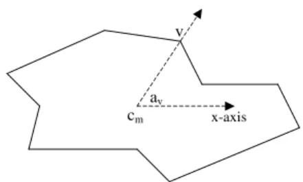
cm x-axis av
v
Fig. 1. Polar Angle Calculations
3 Kinematics-Based Method for Polygon Approximation
KiMPA is applied on polygons in such a way that each vertex of a polygon is associated with an importance level. In fact, the value of the importance level is already encapsulated in the polygon, and kinematics is employed to process that value. The following section presents the preliminary def-initions to clarify the method.
3.1 Preliminaries
Definition 1. (Vertex Velocity) The velocity Vv of a vertex v = (x, y) is
the rate of change of distance per angle.
Definition 2. (Vertex Acceleration) The acceleration Av of a vertex v = (x, y), is the rate of change of velocity per angle.
Vv = ∆d∆av v
, Av = ∆V∆av v
(1)
In Equation (1), d denotes the distance between v and the centroid1 c
m,
av denotes the polar angle of v (cf., Fig. 1).
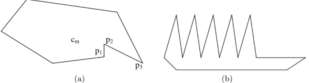
The key observation is as follows: the more the velocity for a vertex, the more sharp the polygon at that vertex. Hence, in order to get a good approximation for the polygonal region, the sharp features should be included. For example in Fig. 2 (a), it would be a better choice to include the points p2 and p3 in the result set rather than including p1 and p2, if one of these three vertices has to be eliminated. In order to differentiate between the vertices, all of them have to be sorted with respect to their velocities and accelerations. The first step is selecting the top-K vertices in the descending velocity order. If the number K is not specified by the user, the default value 2 × |PA| can be used. Among the K vertices, the
top-|PA| vertices are selected as the vertices of the approximated polygon |PA|. By processing the vertices in this manner, the most accelerated (the
most ‘important’) vertices appear in the approximated polygon since they are the vertices where the original polygon has its sharp features.
p1 p2
p3 cm
(a) (b)
Fig. 2. (a) KiMPA Calculations to Detect Sharpness. (b) Visualizing Sharpness on a Comb-like Object.
1 The centroid, or center of mass, of a polygon can be computed as the mean of the
In order to visualize the sharpness on objects, Fig. 2 (b) shows a fluctuating and sharp comb-like figure. This fluctuating and sharp vertices of the polygons can be detected by the change of the acceleration between consecutive vertices. As in the comb-like example, if one extreme has a positive acceleration, the other extreme will have a negative one, leading to a huge acceleration difference between two vertices. Therefore, among these most accelerated points, the very first vertices have to be selected as the final output to have a good approximation.
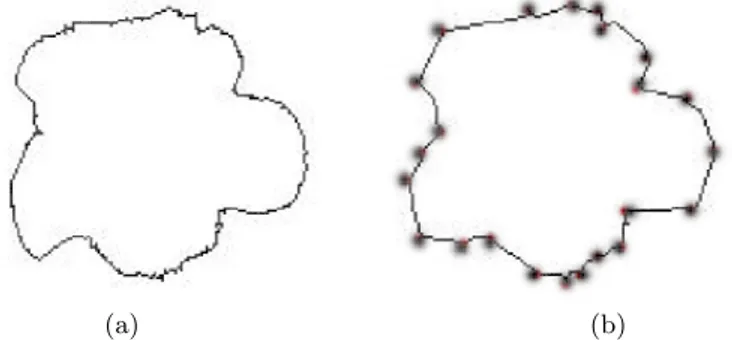
As an example for the KiMPA approximation, Fig. 3 shows a sample polygon corresponding to a rose object. In Fig. 3 (a), the original object is shown as a polygon of 360 vertices. After applying KiMPA method on the object, the object is simplified to 23 vertices as shown in Fig. 3 (b).
(a) (b)
Fig. 3. Application of KiMPA on an input polygon. (a) Original polygon having 360 vertices (at each degree). (b) Polygon after simplification to 23 vertices with K = 64.
3.2 KiMPA Algorithm
The section gives an algorithmic discussion on KiMPA based on the above preliminaries. As mentioned in the problem definition, the input is a set of vertices V corresponding to a polygon. In a polygon, the vertex are in order and this vertex ordering is needed in some calculations of the algorithm. In order to determine the importance levels of the vertices, vertex velocities have to be calculated first. Then, the vertex accelerations can be computed from the vertex velocities. One important point is that the sign of the vertex accelerations has to be taken into consideration. In both of these calculations, the previous vertex of a vertex, according to the initial sorted polar angle ordering, is needed. At the end of this calculation process, the importance level hidden in the vertices are determined.
To continue approximation, the top-K vertices with higher velocities are selected. Then, among these vertices, the most accelerated vertices
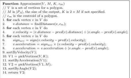
to be in the approximated form are selected. These operations require two sorting operations on the vertex list (in fact the second one is on a much smaller set), and since the final output must be a polygon, one more sorting operation is required to represent the output as a polygon. The overall approximation algorithm is shown in Fig. 4. In the algorithm, a vertex data structure is assumed to have fields for storing distance, velocity, and acceleration.
Function Approximate(V , M , K, cm)
// V is a set of vertices for a polygon.
// M is |PA|, the size of the output, K is 2 × M if not specified.
// cmis the centroid of a polygon.
1. for each vertex v in V do
2. v.distance = findDistance(v, cm);
3. for each vertex v in V do
4. v.velocity = |v.distance − pred(v).distance| ÷ |v.angle − pred(v).angle|;
5. for each vertex v in V do
6. signacc= sign(v.velocity − pred(v).velocity);
7. v.acceleration = signacc× (v.velocity − pred(v).velocity);
8. v.acceleration = v.acceleration ÷ |v.angle − pred(v).angle|;
9. sortByVelocity(V ); 10. V 1 = pickVertices(V, K); 11. sortByAcceleration(V 1); 12. V 2 = pickVertices(V 1, M ); 13. sortByAngle(V 2); 14. return V 2;
Fig. 4. The KiMPA Algorithm
The running time analysis of KiMPA algorithm is as follows: For a polygon, sorting by polar angles may be required and it can be handled in O(|V |log|V |) time. The running time of Approximate() function is dominated by line 9, which is O(|V |log|V |). The first three for loops require O(|V |) time, the other sort operations in line 11 and 13 require O(K) and O(M ) time, respectively. Therefore, KiMPA approximation algorithm takes O(|V |log|V |) time for an arbitrary set of vertices V .
4 Experiments
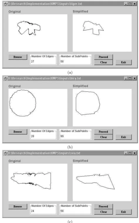
The experiments are based on polygonal objects extracted by our Object Extractor tool [13], which extracts polygonal boundaries of the objects of interest. The tool is a part of the rule-based video database management system that is developed for storing and retrieving video related data and querying that data based on spatio-temporal, semantic, color and shape
(a)
(b)
(c)
Fig. 5. Simplification Experiments on Objects Extracted by Object Extractor (a) tiger, (b) bicy, and (c) sea.
information [2, 3]. It should be noted that an extracted object has at least one vertex (on the boundary) corresponding to every angle with respect to its centroid. Hence, the polygon has at least 360 sides. However, this number is quite large. For example, if we are to use the extracted objects for shape similarity via Turning Angle (TA) method [1], an appropri-ate polygon size is around 20, and it is certain that an approximation is needed. Obviously, randomly selecting the vertices to be in the approxi-mated form would not be the correct way, thus an approximation method preserving the most important vertices is required.
The basic observation for such an experiment is as follows: each vertex on the polygon corresponds to exactly one degree. The vertex velocity of a vertex v is the difference of the distances between v and its predecessor vertex (pred(v)). Similarly, the vertex acceleration of v is the difference between the velocities of v and pred(v). In both of the cases, pred(v) is located in one degree distance from v with respect to the centroid cm.
The results of approximations for a set of polygonal objects are shown in Fig. 5. Since these objects are extracted from digitized images, the critical shape information about the original object is preserved in the approximated polygon. The approximated polygon can be used in pattern recognition [1] and object-based similarity [14] applications.
5 Conclusion
In this paper, a kinematics-based method for polygon approximation, called KiMPA, is proposed. The algorithm is especially suitable for ex-tracting and representing the boundaries of salient objects from video frames for shape-based querying in multimedia, especially video, databases. The polygons are simplified according to the vertex velocities and vertex accelerations with respect to the centroid of the polygon. Velocity and ac-celeration values for vertices are used to express the level of importance, and during vertex elimination the ones having higher importance are pre-served. Since polygon approximation is aimed to overcome the difficulties in processing polygons with a large number of vertices, not only to handle their large memory usage and disk requirements but also to reduce noise, KiMPA can be used to approximate a polygon while preserving the cru-cial information on the polygon. Thus, it can be successfully used within information systems requiring an approximated polygonal representation. While using the algorithm, the user may specify the number of vertices to be in the approximated polygon. Besides, the simplification algorithm may be hierarchically applied, enabling the approximation of a polygon
to a desired simplification level. The method can be integrated to any system and may improve the performance of the approximation. We have conducted several polygon approximations on polygonal objects and the results of these approximations are presented. The results show that the method is successful in approximation of polygonal objects, and provides a way of representing the object with less number of vertices.
References
1. E. Arkin, P. Chew, D. Huttenlocher, K. Kedem, and J. Mitchel. An efficiently computable metric for comparing polygonal shapes. IEEE Transactions on Pattern
Analysis and Machine Intelligence, 13(3):209–215, 1991.
2. M.E. D¨onderler, ¨O. Ulusoy, and U. G¨ud¨ukbay. A rule-based approach to repre-sent spatio-temporal relations in video data. In T. Yakhno, editor, Advances in
Information Sciences (ADVIS’2000), volume 1909 of LNCS, pages 248–256, 2000.
3. M.E. D¨onderler, ¨O. Ulusoy, and U. G¨ud¨ukbay. A rule-based video database system architecture, to appear in Information Sciences, 2002.
4. D. Eu and G.T. Toussaint. On approximating polygonal curves in two and three dimensions. CVGIP: Graphical Models and Image Processing, 56(3):231–246, 1994. 5. M. Garland and P. S. Heckbert. Surface simplification using quadric error metrics.
ACM Computer Graphics, 31(Annual Conference Series):209–216, 1997.
6. S. Grumbach, P. Rigaux, and L. Segoufin. The DEDALE system for complex spatial queries. Proceedings of ACM SIGMOD Symp. on the Management of Data, pages 213–224, 1998.
7. J.D. Hobby. Polygonal approximations that minimize the number of inflections. In Proceedings of Fourth ACM-SIAM Symposium on Discrete Algorithms, pages 93–102, 1993.
8. J. Kim, A.C. Bovik, and B.L. Evans. Generalized predictive binary shape coding using polygon approximations. Signal Processing: Image Communication, 15(7-8):643–663, 2000.
9. Y. Kurozumi and W.A. Davis. Polygonal approximation by the minimax method.
Computer Graphics and Image Processing, 19:248–264, 1982.
10. C.C. Lu and J.G. Dunham. Hierarchical shape recognition using polygon approx-imation and dynamic alignment. Proceedings of 1988 IEEE International
Confer-ence on Acoustic, Speech and Signal Processing, Vol. II, pages 976–979, 1988.
11. J.R. Rossignac and P. Borrel. Multiresolution 3d approximations for rendering complex scenes. In B. Falcidieno and T. Kunii, editors, Modeling in Computer
Graphics: Methods and Applications, pages 455–465, 1993.
12. J. Russ. The Image Processing Handbook. CRC Press, in cooperation with IEEE Press, 1999.
13. E. S¸aykol, U. G¨ud¨ukbay, and ¨O. Ulusoy. A semi-automatic object extraction tool for querying in multimedia databases. In S. Adali and S. Tripathi, editors, 7th
Workshop on Multimedia Information Systems MIS’01, Capri, Italy, pages 11–20,
2001.
14. E. S¸aykol, U. G¨ud¨ukbay, and ¨O. Ulusoy. A histogram-based approach for object-based query-by-shape-and-color in multimedia databases. Technical Report BU-CE-0201, Bilkent University, 2002.
15. W. J. Schroeder, J. A. Zarge, and W. E. Lorensen. Decimation of triangle meshes.