Novel Methods for Microscopic Image Processing,
Analysis, Classification and Compression
a thesis
submitted to the department of electrical and
electronics engineering
and the graduate school of engineering and science
of bilkent university
in partial fulfillment of the requirements
for the degree of
doctor of philosophy
By
Alexander Suhre
March 2013
I certify that I have read this thesis and that in my opinion it is fully adequate, in scope and in quality, as a thesis for the degree of Doctor of Philosophy.
Prof. Dr. Ahmet Enis C¸ etin (Supervisor)
I certify that I have read this thesis and that in my opinion it is fully adequate, in scope and in quality, as a thesis for the degree of Doctor of Philosophy.
Prof. Dr. Orhan Arıkan
I certify that I have read this thesis and that in my opinion it is fully adequate, in scope and in quality, as a thesis for the degree of Doctor of Philosophy.
Assoc. Prof. Dr. U˘gur G¨ud¨ukbay
I certify that I have read this thesis and that in my opinion it is fully adequate, in scope and in quality, as a thesis for the degree of Doctor of Philosophy.
Asst. Prof. Dr. Pınar Duygulu-S¸ahin
I certify that I have read this thesis and that in my opinion it is fully adequate, in scope and in quality, as a thesis for the degree of Doctor of Philosophy.
Assoc. Prof. Dr. Aydın Alatan
Approved for the Graduate School of Engineering and Science:
Prof. Dr. Levent Onural
ABSTRACT
Novel Methods for Microscopic Image Processing,
Analysis, Classification and Compression
Alexander Suhre
Ph.D. in Electrical and Electronics Engineering
Supervisor: Prof. Dr. Ahmet Enis C
¸ etin
March 2013
Microscopic images are frequently used in medicine and molecular biology. Many interesting image processing problems arise after the initial data acquisition step, since image modalities are manifold. In this thesis, we developed several algorithms in order to handle the critical pipeline of microscopic image stor-age/compression and analysis/classification more efficiently.
The first step in our processing pipeline is image compression. Microscopic images are large in size (e.g. 100K-by-100K pixels), therefore finding efficient ways of compressing such data is necessary for efficient transmission, storage and evaluation.
We propose an image compression scheme that uses the color content of a given image, by applying a block-adaptive color transform. Microscopic images of tissues have a very specific color palette due to the staining process they undergo before data acquisition. The proposed color transform takes advantage of this fact and can be incorporated into widely-used compression algorithms such as JPEG and JPEG 2000 without creating any overhead at the receiver due to its
DPCM-like structure. We obtained peak signal-to-noise ratio gains up to 0.5 dB when comparing our method with standard JPEG.
The next step in our processing pipeline is image analysis. Microscopic im-age processing techniques can assist in making grading and diagnosis of imim-ages reproducible and by providing useful quantitative measures for computer-aided diagnosis. To this end, we developed several novel techniques for efficient feature extraction and classification of microscopic images.
We use region co-difference matrices as inputs for the classifier, which have the main advantage of yielding multiplication-free computationally efficient algo-rithms. The merit of the co-difference framework for performing some important tasks in signal processing is discussed. We also introduce several methods that estimate underlying probability density functions from data. We use sparsity criteria in the Fourier domain to arrive at efficient estimates. The proposed methods can be used for classification in Bayesian frameworks. We evaluated the performance of our algorithms for two image classification problems: Dis-criminating between different grades of follicular lymphoma, a medical condition of the lymph system, as well as differentiating several cancer cell lines from each another. Classification accuracies over two large data sets (270 images for follic-ular lymphoma and 280 images for cancer cell lines) were above 98%.
Keywords: Image compression, feature extraction, pattern recognition, kernel
¨
OZET
M˙IKROSKOP˙IK ˙IMGE ˙IS
¸LEME, ANAL˙IZ, SINIFLANDIRMA
VE SIKIS
¸TIRMA ˙IC
¸ ˙IN YEN˙I Y ¨
ONTEMLER
Alexander Suhre
Elektrik ve Elektronik M¨
uhendisli˘
gi B¨
ol¨
um¨
u Doktora
Tez Y¨
oneticisi: Prof. Dr. Ahmet Enis C
¸ etin
Mart 2013
Mikroskopik imgeler tıp biliminde ve molek¨uler biyoloji alanında sıklıkla kul-lanılır. ˙Imge ¨ozellikleri de˘gi¸skenlik g¨osterdi˘gi i¸cin de pek ¸cok ilgi ¸cekici imge i¸sleme problemleri ortaya ¸cıkar. Bu tezde, mikroskopik imge depolama/sıkı¸stırma ve analiz/sınıflandırma s¨urecini ele almak i¸cin bazı algoritmalar geli¸stirdik.
S¨urecimizdeki ilk adım imge sıkı¸stırmadır. Mikroskopik imgelerin boyut-ları b¨uy¨ukt¨ur (¨orne˘gin 100K’ya 100K piksel). Dolayısıyla da, bu imgelerin ver-imli bir ¸sekilde iletimi, saklanması ve de˘gerlendirilebilmesi i¸cin etkin sıkı¸stırma y¨ontemlerinin geli¸stirilmesi gereklidir.
Verilen bir imgenin renk i¸ceri˘gini kullanarak blok-uyarlamalı renk d¨on¨u¸s¨um¨u uygulayan bir imge sıkı¸stırma y¨ontemi ¨oneriyoruz. Veri ediminden ¨once uygu-lanan boyama s¨ureci sebebiyle dokuların mikroskopik imgeleri kendine ¨ozg¨u bir renk paletine sahiptir. ¨Onerdi˘gimiz renk d¨on¨u¸s¨um¨u bu ¨ozellikten faydalanır ve JPEG ya da JPEG 2000 gibi yaygın olarak kullanılan sıkı¸stırma algoritmalarına eklenebilir. Bu ekleme alıcıda DPCM’e benzer yapısı y¨uz¨unden ek bir y¨uk ge-tirmez. Bu y¨ontemle, standart JPEG ile kıyaslayınca sinyal-g¨ur¨ult¨u oranında 0.5 dB’ye varan miktarda artı¸s elde ettik.
S¨urecimizdeki sonraki adım imge analizidir. Mikroskopik imge i¸sleme teknikleri imgelerin sınıflandırmasını ve i¸slenmesini tekrarlanabilir kılar ve bil-gisayar destekli te¸shiste faydalı sayısal ¨ol¸cekler sa˘glar. Bu ama¸cla, etkili ¨oznitelik ¸cıkarma ve mikroskopik imge sınıflandırılması i¸cin ¸ce¸sitli yeni teknikler geli¸stirdik.
Burada ¸carpma gerektirmeyen, hesaplama a¸cısından verimli algoritmalar kul-lanma avantajını sa˘glayan, alan tabanlı e¸s-farklılık matrislerini sınıflandırıcıya girdi olarak verme y¨ontemini kullanıyoruz. E¸s-farklılık matrisleri ¸cer¸cevesinin, i¸saret i¸slemedeki temel bir takım i¸slerin yapılmasındaki ¨onemini tartı¸sıyoruz. Ayrıca altta yatan olasılık yo˘gunluk fonksiyonlarını veriden tahmin eden bir takım y¨ontemler ¨oneriyoruz. Fourier d¨uzlemindeki seyreklik kriterlerini etkili tahminlere ula¸smakta kullanıyoruz. ¨Onerdi˘gimiz y¨ontemler Bayes ¸cer¸cevesinde sınıflandırma i¸cin kullanılabilir. Algoritmalarımızın performansını iki imge sınıflandırma probleminde de˘gerlendirdik: Folik¨uler lenfomanın farklı derecelerini ayırt etmek ve bir takım kanser h¨ucre dizilerini birbirinden ayırmak. ˙Iki b¨uy¨uk veri setinde (folik¨uler lenfoma i¸cin 270 imge ve kanser h¨ucre dizileri i¸cin 280 imge) sınıflandırma do˘grulu˘gu %98’in ¨uzerindedir.
Anahtar Kelimeler: imge sıkıstırma, ¨oznitelik ¸cıkarımı, ¨or¨unt¨u tanıma, ¸cekirdek
ACKNOWLEDGMENTS
As John Donne once said: “No man is an island.” The following people have been indispensable to the learning process I underwent during my time in graduate school. I would like to thank
• My supervisor A. Enis C¸etin for supporting me in every possible way. • Orhan Arıkan and U˘gur G¨ud¨ukbay for their valuable feedback during the
work on this thesis.
• Pınar Duygulu S¸ahin and Aydın Alatan for agreeing to be on my defense
committee.
• Levent Onural for giving me the chance to start graduate school at Bilkent
University.
• Ergin Atalar for his help when the going got tough.
• Reng¨ul C¸etin-Atalay for giving me the opportunity to work in the field of
microscopic images.
• The Scientific and Technological Research Council of Turkey (T¨UB˙ITAK)
for my scholarship.
• The European Commission and its IRSES Project 247091 MIRACLE for
• My office mates during the first years of my Ph.D., for helping me adjust to
the new environment and thereby teaching me many things. I will always be indebted to G¨okhan Bora Esmer, Fahri Yara¸s, Erdem Ulusoy, Ali ¨Ozg¨ur Y¨ontem and Erdem S¸ahin.
• Kıvan¸c K¨ose and his wonderful wife Bilge for being just the way they are. • Ay¸ca ¨Oz¸celikale and Mehmet K¨oseo˘glu for their friendship during hard
times and the delicious fruit.
• M¨ur¨uvet Parlakay for her tireless efforts and good humor.
• M. Furkan Keskin and T¨ulin Er¸sahin for their collaboration on many
ex-periments.
• All members of the Signal Processing Group Bilkent past and present:
Beh¸cet U˘gur T¨oreyin, Osman G¨unay, Serdar C¸ akır, Onur Yorulmaz, Alican Bozkurt, ˙Ihsan ˙Ina¸c, Y. Hakan Habibo˘glu, Ahmet Yazar, R. Akın Sevimli, Fatih Erden, Kaan Duman, Onay Urfalio˘glu and Kasım Ta¸sdemir.
• All the good people I met in Ankara: Zeynep Y¨ucel, Elif Aydo˘gdu, Aslı
¨
Unl¨ugedik, G¨ulis Zengin, Can Uran, Esra Abacı-T¨urk & Ata T¨urk, S. Figen ¨
Oktem, Ezgi S¸afak, Teksin Acıkg¨oz Kopano˘glu & Emre Kopano˘glu, Aydan Ercing¨oz, Sıla T¨urk¨u Kural ¨Unal & Alper ¨Unal, G¨ok¸ce Balkan, M. Can Kerse, Sinan Ta¸sdelen, Yi˘gitcan Eryaman, A. Serdar Tan, Namık S¸engezer, Volkan H¨unerli, Merve ¨Onenli G¨uven & Volkan G¨uven, Anirudh Srinivasan, Nurdane ¨Oz, Deniz Atasoy, Simon Sender, Kevin Kusmez & G¨uls¨um ¨Ozsoy Kusmez, Natalie Rizzuto and Julie Shaddox for the good times and many laughs.
• John Angliss for reminding me from time to time that there is more. • Sibel Kocao˘glan for trying all she could to keep me sane.
• Marshall Govindan and Shibendu Lahiri for their advice and insights. • Christian Hahn for “keepin’ it real”.
• My parents Leonie & R¨udiger as well as the rest of my family for their love
and understanding.
Last but not least, my heart goes out to Yufang Sun. Her love and friendship have sustained me throughout these challenging times.
Contents
1 INTRODUCTION 1
1.2 Microscopic Image Compression . . . 3
1.3 Microscopic Image Analysis . . . 4
1.3.1 Feature Extraction . . . 5
1.4 Microscopic Image Classification . . . 6
1.4.1 Follicular Lymphoma Classification Using Sparsity Smooth-ing . . . 7
1.4.2 Bandwidth Selection in Kernel Density Estimation using Fourier Domain Constraints . . . 8
1.4.3 Image Thresholding using Mixtures of Gaussians . . . 9
1.4.4 Cancer Cell Line Classification using Co-Difference Oper-ators . . . 10
2 MICROSCOPIC IMAGE COMPRESSION 13 2.1 Algorithm . . . 16
3 CLASSIFICATION OF FOLLICULAR LYMPHOMA IMAGES BY REGION COVARIANCE AND A BAYESIAN CLASSI-FIER USING SPARSITY IN TRANSFORM DOMAIN 39
3.1 Feature Extraction . . . 42
3.2 Classification . . . 45
3.2.1 First classification stage . . . 45
3.2.2 Second classification stage . . . 45
3.3 Experimental Results . . . 49
4 BANDWIDTH SELECTION IN KERNEL DENSITY ESTI-MATION USING FOURIER DOMAIN CONSTRAINTS 54 4.1 CV-based cost function for Bandwidth Estimation . . . 57
4.1.1 Cross-validation using l1 Norm in Fourier Domain . . . 58
4.1.2 Cross-validation using l1 Norm and Filtered variation . . . 59
4.2 Simulation Results . . . 60
5 IMAGE THRESHOLDING USING MIXTURES OF GAUS-SIANS 77 5.1 Description of the Algorithm . . . 78
5.1.1 Bandwidth choice of the Gaussian kernel . . . 80
6 CANCER CELL LINE CLASSIFICATION USING
CO-DIFFERENCE OPERATORS 91
6.1 Vector Product and Image Feature Extraction Algorithm . . . 92
6.2 Experimental results . . . 95
6.2.1 Feature Extraction . . . 97
List of Figures
2.1 A general description of our prediction scheme. To predict the color content of the black-shaded image block, color contents of previously encoded gray-shaded blocks, marked by arrows, are used. Figure reproduced from Reference [1] with permission. . . . 21
2.2 PSNR-vs-CR performance of the ‘24’ image from the Kodak dataset for fixed color transforms and the color weight method. (a) Original Image, (b) Rate-Distortion curve. Our method out-performs the baseline transforms. Figure reproduced from Refer-ence [1] with permission. . . 26
2.3 PSNR-vs-CR performance of the ‘23’ image from the Kodak dataset for fixed color transforms and the color weight method. (a) Original Image, (b) Rate-Distortion curve. The baseline trans-forms outperform our method. Figure reproduced from Refer-ence [1] with permission. . . 27
2.4 PSNR-vs-CR performance of the ‘Lenna’ image for fixed color transforms and the color weight method. (a) Original Image, (b) Rate-Distortion curve. Our method outperforms the baseline transforms. Figure reproduced from Reference [1] with permission. 28
2.5 PSNR-vs-CR performance of the ‘01122182-0033-rgb’ image (sec-ond image in microscopic image dataset) for fixed color trans-forms and the color weight method. (a) Original Image, (b) Rate-Distortion curve. Our method outperforms the baseline trans-forms. Figure reproduced from Reference [1] with permission. . . 29
2.6 A visual result of image ‘24’ from the Kodak dataset coded by JPEG using a quality factor of 80%. (a) Original, (b) JPEG coded version using Y’CbCr and (c) JPEG coded version using the color weight method with Y’CbCr. Figure reproduced from Reference [1] with permission. . . 30
2.7 Example of the segmentation using the algorithm described in Chapter 4. (a) shows the original image 1 from the microscopic image dataset and (b) shows the segmentation, where white pixels denote background and black pixels denote foreground. Original image repoduced from Reference [2] with permission. . . 37
3.1 Examples of FL images used in this study: (a) FL grade 1, (b) FL grade 2 and (c) FL grade 3 . . . 41
3.2 Examples of of the Hp and Ep for the grade 3 image of Figure 3.1
(c): (a) Hp, (b) Ep . . . 43
3.3 The procedure of the proposed FL classification method. . . 44
3.4 Examples of the histograms of L (right) and Hp (left) used in the
first step of classification: (a) FL grade 1, (b) FL grade 2, (c) FL grade 3. . . 46
3.5 Depiction of the algorithm described in Section 3.2. The histogram in (a) which has empty bins is transformed into (b) using DCT. In (c) the values of the high frequency coefficients are set to zero. The inverse DCT of (c) yields an estimate for the likelihood function that has only non-empty bins, see (d). Note that in (d), bins may have very small likelihood values but larger than zero. Figure reproduced from Reference [3] with permission. . . 50
4.1 Estimated σ for Sheather’s method and the proposed method. . . 67
4.2 Results of KDE for 15 example distributions used in this chap-ter. Shown are the original (black), KDE with Sheather’s method (blue) and KDE with the proposed method cross validation (red) and the proposed cross validation with l1 norm term and filter
(green). . . 76
5.1 An illustration of the algorithm. The figure shows the final stage of the algorithm. Bin 4 is assigned to cluster U and the algorithm is aborted. . . 80
5.2 Example in which our method performed better than Otsu’s method according to five out of six metrics: (a) image 6 from the dataset, (b) its groundtruth segmentation, (c) our proposed segmentation and (d) Otsu’s segmentation. . . 84
5.3 Example in which our method performed worse than Otsu’s method according to three out of six metrics: (a) image 2 from the dataset, (b) its groundtruth segmentation, (c) our proposed segmentation and (d) Otsu’s segmentation. . . 85
5.4 Example in which our method performed worse than Otsu’s method according to five out of six metrics: (a) image 47 from the dataset, (b) its groundtruth segmentation, (c) our proposed segmentation and (d) Otsu’s segmentation. . . 86
5.5 Example of a possible application area: (a) cropped cell image from the BT-20 cancer cell line, (b) our proposed segmentation and (c) Otsu’s segmentation. . . 87
5.6 Example of a possible application area: (a) cropped cell image from the BT-20 cancer cell line, (b) our proposed segmentation and (c) Otsu’s segmentation. . . 88
5.7 Example of a possible application area: (a) cropped cell image from a BT-20 cancer cell line, (b) our proposed segmentation and (c) Otsu’s segmentation. . . 89
5.8 Example of a possible application area: (a) cropped cell image from the BT-20 cancer cell line, (b) our proposed segmentation and (c) Otsu’s segmentation. . . 90
6.1 Examples of the image classes used in our experiments. Figure reproduced from Reference [4] with permission. . . 102
List of Tables
2.1 The condition numbers of the baseline transforms and the mean and standard deviations of the condition number of our transforms for the Kodak dataset. . . 19
2.2 Mean and standard deviations of the correlation coefficients ρij
for the baseline color transforms and our transforms as computed over the Kodak dataset. . . 20
2.3 PSNR-Gain values for the whole dataset with different baseline color transform. PSNR-Gain of each image is measured at differ-ent rates and averaged. α is equal to 2.5. . . . 24
2.4 PSNR-Gain values for the whole dataset with different baseline color transform. PSNR-Gain of each image is measured at differ-ent rates and averaged. α is equal to 3. . . . 25
2.5 PSNR-Gain values for the whole dataset with different baseline color transform. PSNR-Gain of each image is measured at differ-ent rates and averaged. α is equal to 2. . . . 25
2.6 PSNR-Gain values for the whole dataset with different baseline color transform. PSNR-Gain of each image is measured at differ-ent rates and averaged. No threshold was used, i.e. the whole image was coded with our method. . . 25
2.7 PSNR-Gain values for the whole microscopic image dataset with different baseline color transform. PSNR-Gain of each image is measured at different rates and averaged. α is equal to 2.5. . . . . 32
2.8 PSNR-Gain values for the whole microscopic image dataset with different baseline color transform. PSNR-Gain of each image is measured at different rates and averaged. α is equal to 3. . . . 33
2.9 PSNR-Gain values for the whole microscopic image dataset with different baseline color transform. PSNR-Gain of each image is measured at different rates and averaged. α is equal to 2. . . . 34
2.10 PSNR-Gain values for the whole microscopic image dataset with different baseline color transform. PSNR-Gain of each image is measured at different rates and averaged. No threshold was used, i.e. the whole image was coded with our method. . . 35
2.11 PSNR-Gain values for the whole microscopic image dataset us-ing the KDE segmentation of this section. The parameter a was chosen as 0.99. . . 38
3.1 Image recognition rates (%) for all three grades and two classifiers different classifiers in the second stage: The proposed sparsity smoothing and SVM. . . 51
3.2 Mean and standard deviations of block recognition rates (%) for grades 1 and 2 and two different classifiers in the second stage: The proposed sparsity smoothing and SVM. . . 52
3.3 Mean and standard deviations of Kullback-Leibler divergence for test images from Grade 1 to the training images of class A (grade 1 and 2) and class B (grade 3) with L and Hp features. . . 52
3.4 Mean and standard deviations of Kullback-Leibler divergence for test images from grade 2 to the training images of class A (grade 1 and 2) and class B (grade 3) with L and Hp features. . . 52
3.5 Mean and standard deviations of Kullback-Leibler divergence for test images from Grade 3 to the training images of class A (grade 1 and 2) and class B (grade 3) with L and Hp features. . . 53
4.1 KL divergence gain in dB over Sheather’s method for traditional cross-validation . . . 62
4.2 MISE gain in dB over Sheather’s method for traditional cross-validation. . . 62
4.3 KL divergence gain in dB over Sheather’s method for proposed cross-validation with l1 term. . . 63
4.4 MISE gain in dB over Sheather’s method for proposed cross-validation with l1 term. . . 63
4.5 KL divergence gain in dB over Sheather’s method for proposed cross-validation with l1 term. wh[n] was used. . . . 64
4.6 MISE gain in dB over Sheather’s method for proposed cross-validation with l1 term. wh[n] was used. . . . 64
4.7 KL divergence gain in dB over Sheather’s method for proposed cross-validation with l1 term. wl[n] was used. . . . 65
4.8 MISE gain in dB over Sheather’s method for proposed cross-validation with l1 term. wl[n] was used. . . . 65
4.9 KL divergence gain in dB over Sheather’s method for proposed cross-validation with l1 term. wq[n] was used. . . . 66
4.10 MISE gain in dB over Sheather’s method for proposed cross-validation with l1 term. wq[n] was used. . . . 66
5.1 Differences between Otsu’s method and our proposed method for different distance metrics according to Equation (5.7). A posi-tive value indicates that our method had a lower score and was therefore better than Otsu’s method. The last row denotes the percentage of images in the dataset where our proposed methods outperforms Otsu’s method. . . 82
5.2 Differences between Otsu’s method and our proposed method for different distance metrics according to Equation (4.14). A posi-tive value indicates that our method had a lower score and was therefore better than Otsu’s method. The last row denotes the percentage of images in the dataset where our proposed methods outperforms Otsu’s method. . . 83
6.1 Covariance vs. co-difference computational cost. The fourth col-umn shows the ratio of the second and third colcol-umn, respectively. 94
Chapter 1
INTRODUCTION
”He is an optician, daily having to deal with the microscope, tele-scope, and other inventions for sharpening our natural sight, thus enabling us mortals (as I once heard an eccentric put it) liberally to enlarge the field of our essential ignorance.”
Herman Melville, Inscription Epistolary to W. Clark Russell
Vision is arguably one of the most important senses that human beings rely on. However, human vision has only limited resolution and bandwidth. To overcome these limitations has been a steady endeavor of science and engineering from its very beginnings.
The origins of microscopy can be traced back as far as the year 1000 with the first descriptions of concave and convex lenses. In 1595, William Borel delivered the first description of a compound microscope built by the Dutch spectacle-maker Hans Jansen and his son Zacharias. The first detailed scientific study of microscopy dates back to Robert Hooke’s milestone book ”Micrographia” in 1665 [5]. In 1873, Abbe published his landmark paper [6], finding the relation of the smallest resolvable distance between two points given the wavelength of the imaging light when using a conventional microscope. This diffraction limit
was accepted as the ruling paradigm for imaging until the introduction of sub-diffraction imaging in the early 2000s [7]. Abbe’s findings were instrumental in developing the first fluorescent microscope in 1911 by Oskar Heimstaedt [8]. In 1935, Frits Zernike discovered the principle of phase contrast [9]. The advent of the confocal microscope in 1961 [10] allowed researchers to witness a new level of optical resolution. Confocal microscopy can also be used for three-dimensional reconstruction of the sample [11]. Of special interest for image processing prac-titioners may be the deconvolution-type algorithms in microscopy [12]. An in-formative overview of the milestones of microscopy is provided in [13].
To illustrate the scope of this thesis, let us first discuss what it is not. This thesis does not deal with the actual image acquisition process of microscopic images. Data was provided by collaborators, e.g., the molecular biology depart-ment of Bilkent University, using state-of-the-art imaging systems. The problems that will be adressed in this thesis are therefore issues that arise after imaging and mostly deal with the analysis of the information contained in the images at hand, i.e., the whole processing pipeline of microscopic images, consisting of compression, analysis and classification.
Depending on the sample under observation, we will deal with a large variety of image modalities, from which a variety of image processing problems arise. Example images are shown in Figures 2.2 (a), 3.1 and 6.1. We ask the following question: Can the specific features of microscopic images, such as color con-tent and morphology be used for more efficient compression and classification? The short answer is a resounding “yes”. The long answer will be given in the remainder of this thesis.
1.2
Microscopic Image Compression
As the amount of digitally stored data is increasing rapidly [14], data compres-sion is a topic that needs to be adressed. The National Institute of Health (NIH) in America issued a call for proposals on the problem of compression of micro-scopic image data in April 2009. Recent advances in technology have enabled researchers to digitize pathological whole-slides at high magnifications (e.g. at 40x). Resulting color microscopic images are large in size (e.g. 100K-by-100K). Therefore, finding efficient ways of compressing such data is necessary for efficient transmission, storage and evaluation.
Currently, standard image compression methods such as JPEG or JPEG 2000 are used for microscopic image compression. The DCT-based “lossy” JPEG standard [15] has proven to be the most widely accepted technique in modern day applications, thus making the very term JPEG a household name. JPEG, however, was designed and performs best for so-called “natural” images. For example, it uses color transforms of the YUV flavor, in which the luminance component holds most of the energy, compared to the other two chroma com-ponents. The weighting coefficients in these color transform matrices model the human visual system (HVS). For other, most notably medical, applications this strict assumption on the color content of the given image may not be valid. This is due to the fact that images of tissue are usually stained with certain dyes [16]. For example, tissue samples showing different follicular lymphoma grades are stained using haematoxylin and eosin (H&E) dyes. Haematoxylin stains cell nu-clei blue, while eosin stains cytoplasm, connective tissue and other extracellular substances pink or red. The respective color content of those images is therefore significantly different from the color content of “natural scene” images.
The motivation of our research here is to find an efficient method to represent the color content of a given image in a way that can be integrated with widely
used compression schemes such as JPEG and JPEG 2000. In this thesis, we developed a weight-based color transformation method for microscopic images, that takes the image specific color-content into account and can replace standard color transforms in JPEG and other compression schemes. In the conducted tests the proposed method yielded an increase in PSNR value up to 0.15 dB for natural images and up to 0.5 dB for microscopic images, compared to standard JPEG.
1.3
Microscopic Image Analysis
To this day, analysis of microscopic images of human tissues remains the most reliable way of diagnosing and grading several illnesses, e.g., cancer. Our work on the classification and rating of microscopic images is motivated by the fact that there is significant inter- and intra-rater variability in the grading and diagnosis of these illnesses from image data by human experts. Computer-aided classification can assist the experts in making their grading and diagnosis reproducible, while additionally providing useful quantitative measures.
One of the first applications of computer-aided diagnosis (CAD) was digital mammography in the early 1990’s [17], [18]. CAD has become a part of routine clinical detection of breast cancer on mammograms at many screening sites and hospitals [19] in the United States. Interest in research of medical imaging and diagnostic radiology has increased since then. Given modern day computing re-sources, computer-aided image analysis can play its part in facilitating disease classification. Using CAD makes also sense when considering another issue: It has been estimated that roughly 80% of all yearly prostate biopsies in the U.S.A. are benign [20], which means that pathologists spend a larg amount of their time sieving through benign tissue. If CAD could help pathologists to analyse benign tissue faster, a significant amount of time and money could be saved.
The authors of [20] wrote: “Researchers in both the image analysis and pathol-ogy fields have recognized the importance of quantitative analysis of patholpathol-ogy images. Since most current pathology diagnosis is based on the subjective (but educated) opinion of pathologists, there is clearly a need for quantitative image-based assessment of digital pathology slides.” Applications are in cancer research. Similar techniques can also be used for problems arising in molecular biology.
1.3.1
Feature Extraction
The first step of most image interpretation problems including microscopic im-age processing is feature extraction [21]. Feature vectors represent or summarize a given image. In many problems, image classification is then performed using the feature vectors instead of actual pixel values. Microscopic images are large in size, which requires the feature extraction process to be computationally effi-cient in order not to rely on supercomputers or computer clusters in the future. Furthermore, the proper choice of feature vectors is crucial.
One problem in this context is not to be underestimated: Humans’ concept of the world is inherently object-based, while in image processing we deal with the real world’s pixel-based representation. However, human experts describe and understand images in terms of such rather abstract objects. A pathologist, e.g., will describe his or her diagnosis criteria in terms of notions like “nucleus” and “cell.” Establishing the link between the “object” and its pixel representation in the image is not straight-forward. Research on useful features for disease classification has often been inspired by visual attributes defined by clinicians as particularly important for disease grading and diagnosis. This ultimately means that the image processing specialist has to learn these features from a seasoned pathologist and thereby become similarily well-skilled in pathology. This may involve a long, iterative process. However, model complexity can not be increased endlessly without the risk of overfitting [22]. One may also ask if it is always
wise to try to mimick the process of a pathologist step-by-step or if a set of low-level features paired with an efficient classifier may result in a better performing sytem. We will introduce such an approach in Chapter 3.
One of the most promising feature extraction methods in recent years has been the region covariance method, which was successfully used in image texture classification and object recognition [23]. Region covariance method features are extensively used in texture classification and recognition in image and video. Given a feature vector of an image region, a covariance matrix is constructed, thereby measuring the interplay of the given features. Covariance matrix com-putation for N features is of orderO(N2), due to the extensive number of vector
multiplications involved. As mentioned above, the size of microscopic image data requires the feature extraction process to be computationally efficient. The so-called region co-difference matrices serve the same purposes as region covariance matrices and exhibit similar performance but do no rely on the multiplication op-erator [24]. Texture classification techniques like this can be used for microscopic images to classify them into groups and recognize specific types of diseases. We present frameworks based on these ideas in Chapter 3 (for region covariance) and Chapter 6 (for region co-difference). For a further in-depth review of feature extraction for microscopic images, the reader may consult [20].
1.4
Microscopic Image Classification
After feature extraction has been carried out successfully, classification is per-formed. The problems to be solved can range from binary classification within a given image, e.g., segmentation of pixels into foreground and background, to discrimination of several images into a set of classes. A large amount of literature on classification schemes exists [25]. The Bayes classifier minimises the probabil-ity of misclassification [26], but it requires an estimate of the likelihood function
of the data. However, this function is usually unknown. Histograms of the data can be used for this purpose, but due to the limited amount of data, these will be rather poor estimates of the underlying probability density functions (PDFs). In fact, smoothing the histograms will result in more desirable estimates [27]. We will present several algorithms in order to achieve this task.
1.4.1
Follicular Lymphoma Classification Using Sparsity
Smoothing
The first microscopic image classification problem that we will discuss deals with follicular lymphoma (FL). FL is a group of malignancies of lymphocyte origin that arise from lymph nodes, spleen and bone marrow in the lymphatic system in most cases and is the second most common non-Hodgkin’s lymphoma. FL can be differentiated from all other subtypes of lymphoma by the presence of a follicular or nodular pattern of growth presented by follicle center B cells consisting of cen-trocytes and centroblasts. In practice, FL grading process often depends on the number of centroblasts counted within representative follicles, resulting in three different grades describing the severity of the disease. Although reliable clini-cal risk stratification tools are available for FL, the optimal choice of treatment continues to depend heavily on morphology-based histological grading.
Current microscopic image classification systems for FL consist of follicle tection using immunohistochemical (IHC) images, image registration, follicle de-tection using haematoxylin-eosin (H & E) stained images, centroblast dede-tection, and false positive elimination [28]. Therefore, microscopic image analysis for this disease involves many algorithmic components. Optimal and robust functioning of each of these components is important for the overall accuracy of the final system.
In Chapter 3, a different approach in terms of feature extraction and classi-fication was chosen. The philosophy behind this is the following: Features that pathologists and molcecular biologists are interested in with respect to biomed-ical images are oftentimes hard to model on an image level. If, however, it is known that the feature in question can be decomposed into several low-level com-ponents, but their interplay in a particular instance of a feature may be unknown, the covariance of these features may help in classifying the feature correctly.
In Chapter 3, we wish to classify images of the three different grades of FL. In order to carry out classification of the computed features we need to estimate their underlying likelihood functions. Such functions tend to be smooth functions, i.e., they are sparse in the Fourier domain. We introduce a novel classification algorithm that imposes sparsity on the likelihood estimate in an iterative manner. The transform domain in which we will impose sparsity is the discrete cosine transform (DCT), because of its energy compaction property [29]. Once an estimate of the likelihood function is found, a Bayes classifier can be used for the final classification. Classification accuracies for our proposed methods were above 98% for all three FL grades.
1.4.2
Bandwidth Selection in Kernel Density Estimation
using Fourier Domain Constraints
We believe that using sparsity in PDF estimation can be a powerful tool. In fact a wide range of literature on the issue of sparsity exists, especially within the context of what is commonly referred to as “compressive sensing” (CS) [30]. CS is a technique in which an ill-conditioned system like Ax = b, where A does not have full-rank, can be solved uniquely with high probability. This, however, can only be achieved if the data x is sparse in some basis. One can measure sparsity by computing the signal’s l0 norm. Unfortunately, minimizing
an expression including the l0 norm is non-deterministic polynomial-time (NP)
hard. Therefore, one usually uses the l1 norm as a sparsity restriction for a
minimization.
In Chapter 4, we will not use full CS-type algorithms but we will impose sparsity in the Fourier domain on the PDF estimates for kernel density estimation (KDE), via minimization of the l1 norm. In KDE, a PDF can be estimated from
data using a kernel function, the most popular of which is the Gaussian kernel. A crucial problem here is how to choose the the bandwidth of the kernel or, in case of the Gaussian kernel, its standard deviation σ. In case the σ is chosen too large or too small, the resultant PDF will be over-smoothed or under-smoothed, respectively. In the statistics community, many algorithms have been developed to estimate a proper bandwidth. The common opinion here is that so-called “plug-into-the-equation” type estimators [31] outperform other approaches [32]. These types of algorithms iteratively update their estimates, but initially rely on an estimate from a parametric family, the so-called “pilot estimate”. A concern that is voiced frequently in the statistics community [33] is that the pilot estimate may be computed under wrong assumptions. In this thesis, we are interested in finding approaches to the described problem by using the Fourier domain properties of the data. Similar approaches are to the best of our knowledge absent in the literature. We present an algorithm that outperforms the traditional method by Sheather for different lengths of data. In our simulations the proposed method resulted in Kullback-Leibler divergence gains of up to 2dB.
1.4.3
Image Thresholding using Mixtures of Gaussians
Image segmentation is an important part of image understanding. The most basic problem here is segmentation of the pixels into foreground and background. This is usually accomplished by choosing an appropiate threshold [34]. The resultant binary image can be used as input for more advanced segmentation
algorithms [35]. Therefore, the quality of the final segmentation in that case will largely depend on the initial threshold choice, which is why image thresholding can only be considered a “basic” problem at first sight. In microscopic images, thresholding can be used to find the outline of cell organels within the nucleus. Examples are shown in Figures 5.5-5.8.
In order to estimate a threshold in a simple foreground-background image segmentation problem, mixtures of Gaussians can also be used. To this end we present an algorithm that outperforms the widely used method by Otsu [36] in Chapter 5. Image histogram thresholding is carried out using the likelihood of a mixture of Gaussians. In the proposed approach, a PDF of the data is estimated using Gaussian kernel density estimation in an iterative manner, using the method from Chapter 4. The threshold is found by iteratively computing a mixture of Gaussians for the two clusters. This process is aborted when the current bin is assigned to a different cluster than its predecessor. The method is self-adjusting and does not involve an exhaustive search. Visual examples of our segmentation versus Otsu’s thresholding method are presented. We evaluated the merit of our method on a dataset of 49 images with groundtruth segmentations. For a given metric our proposed method yielded up to 10% better segmentations than Otsu’s method.
1.4.4
Cancer Cell Line Classification using Co-Difference
Operators
Cancer cell lines (CCL) are widely used for research purposes in laboratories all over the world. They represent different generations of cancer cells that are usually grown in a laboratory environment and whose bio-chemical properties are well known. Molecular biologists use CCLs in their experiments for testing the effects of certain drugs on a given form of cancer. However, during those
experiments the identity of the CCLs have to be confirmed several times. The traditional way of accomplishing this is to use short tandem repeat (STR) anal-ysis. This is a costly process and has to be carried out by an expert. Computer-assisted classification of CCLs can alleviate the burden of manual labeling and help cancer research. In Chapter 6, we present a novel computerized method for cancer cell line image classification.
The aim is to automatically classify 14 different classes of cell lines including 7 classes of breast and 7 classes of liver cancer cells. Microscopic images con-taining irregular carcinoma cell patterns are represented by subwindows which correspond to foreground pixels. The images of the CCLs contain a large num-ber of different junctions and corners, whose orientation is random. To quantify these directional variations, a region covariance/co-difference descriptor utiliz-ing the dual-tree complex wavelet transform (DT-CWT) coefficients and several morphological attributes was computed. Directionally selective DT-CWT fea-ture parameters are preferred primarily because of their ability to characterize edges at multiple orientations which is the characteristic feature of carcinoma cell line images. A support vector machine (SVM) with radial basis function (RBF) kernel was employed for final classification. The proposed system can be used as a reliable decision maker for laboratory studies. Our tool provides an automated, time- and cost-efficient analysis of cancer cell morphology to classify different cancer cell lines using image-processing techniques, which can be used as an alternative to the costly STR analysis.
In order to achieve this result, a new framework for signal processing is intro-duced. It is based on a novel vector product definition that permits a multiplier-free implementation. In this framework, a new product of two real numbers is defined as the sum of their absolute values, with the sign determined by the product of the two hard-limited numbers. This new product of real numbers is used to define a similar product of vectors in RN. The new vector product of two
identical vectors reduces to a scaled version of the l1 norm of the vector. The
main advantage of this framework is that it yields multiplication-free computa-tionally efficient algorithms for performing some important tasks in microscopic image processing. This is necessary to achieve an almost-real time processing of microscopic images, where computer-aided analysis can provide results within seconds, compared to minutes when a human being carries out the same task. In research environments, a speed-up on such a scale will help medical doctors or molecular biologists significantly. Over a dataset of 280 images, we achieved an accuracy above 98%, which outperforms the classical covariance-based methods.
Chapter 2
MICROSCOPIC IMAGE
COMPRESSION
Image compression is a well-established and extensively studied field in the sig-nal processing and communication communities. Although the “lossy” JPEG standard [15] is one of the most widely accepted image compression techniques in modern day applications, its resulting fidelity can be improved. It is a well known fact that JPEG compression standard is optimized for natural images. More specifically the color transformation stage is designed in such a way that, it favors the color components to which the human visual system (HSV) is more sensitive in general. However, using one fixed color transformation for all types of natural images or even for all the blocks of an image may not be the most efficient way.
One possible idea is to find a color transform that represents the RGB com-ponents in a more efficient manner and can thereby replace the well-known RGB-to-YCbCr or RGB-to-YUV color transforms, used by most practitioners. Usually such approaches aim at reducing the correlation between the color channels [37]. An optimal solution would be to use Karhunen-Lo`eve Transform (KLT), see [38].
However, in KLT there is an underlying wide-sense stationary random process assumption which may not be valid in natural images. This is because autocor-relation values of the image have to be estimated to construct the KLT matrix, since most natural images cannot be considered as wide-sense stationary random processes, due to edges and different objects. A single auto-correlation sequence cannot represent a given image. Another approach to an optimal color space projection on a four-dimensional colorspace was developed in [39]. The follow-ing literature survey aims at establishfollow-ing today’s state of the art in the area of microscopic image compression for medical purposes.
Okurma et al. [40] studied the characteristics of pathological microscopic images (PMI). Although colorless by nature, sample images are prepared by using special dyes producing color. When comparing these sample images with natural images based on CIE chromaticity diagrams, it was shown that PMI are more concentrated around specific color components than their natural counterparts.
Nakachi et al. [41] developed a full-grown coding scheme for PMI. They avoid the effects of chrominance downsampling by using a Karhunen-Lo`eve Transform (KLT), its main advantages being to reduce correlation between RGB color-components and biasing the signal energy between the transformed color-components. Ladder networks are used to implement KLT. Experiments show that the KL-transformed images have lower entropy than their RGB or YCbCr counterparts. The actual coding process involves a S+P transform followed by a SPIHT coder for each transformed component.
A much larger branch of research activities on efficient coding of medical images involve wavelet approaches to the problem. Ref. [42] offers a clear intro-duction to the field.
Manduca [43] presented a study comparing the performance of JPEG, stan-dard wavelet (using run-length and arithmetic coding) as well as wavelet trans-form followed by a SPIHT coding method. For four different images (‘Lena’, MRI, CT and X-ray) and compression ratios from 10:1 up to 40:1, the RMS errors of the three methods was compared resulting in a distinguishably bet-ter performance of SPIHT, followed by standard wavelet compression and lastly normal JPEG.
Arya et al. [44] use a vector quantisation approach for coding medical image sequences. Using interframe correlation by applying a 3-D vector scheme yields significantly higher PSNR values than baseline H.261 video codec. O˘guz and C¸ etin also used video coders to compress MRI images in the past [45]. Since our research is dedicated to single images and not sequences of such, an approach like this was not further investigated.
Gormish et al. introduced their CREW compression system in [46]. This system is lossless and idempotent, using a customised reversible color transform, a wavelet transform and a quantization via alignment routine, in which the fre-quency bands are ”aligned” following a selectable rule. CREW has a tagged file format, that also contains information about importance levels of certain regions and not only pixel data. Experimental results show a compression gain of about 10% in Bits/Pixel. Note that this study aims not particularily at medical, but general high quality images.
Zamora et al. [47] worked on a particular problem, namely compression of images showing osteoporotic bone. They exploit certain properties of the image data, namely its small variance in color. For that reason run-length coding is a well-suited approach to coding these types of images. Data given by the authors confirms that run-length coding, though quite a simple technique, is competible with adaptive arithmetic coding, which again can achieve entropy values very
close to the input data’s entropy. Assuming a six-color model for the input data compression ratios can go up to 100:1 with low computational effort.
A new transform based on the color content of a given image is developed in this chapter. The proposed transform can be used as part of the JPEG im-age coding standard, as well as part of other imim-age and video coding methods, including the methods described in [48], [49] and [50].
2.1
Algorithm
A typical colorspace transform can be represented by a matrix multiplication as
follows: D E F = T· R G B , (2.1)
where T = [tij]3×3 is the transform matrix, while R, G and B represent the
red, green and blue color components of a given pixel, respectively, and D, E, F represent the transformed values, see [51] and [52]. For example, JPEG uses luminance-chrominance type colorspace transforms and chooses the coefficients in T accordingly. Examples for these include RGB-to-YCbCr [53], as definded in JPEG File Interchange Format (JFIF), as well as RGB-to-YUV and a digital version of RGB-to-Y’CbCr from CCIR 601 Standard that are used in our ex-periments as baseline color transforms. Their respective transform matrices are given by T′RGB−to−Y CbCr = 0.299 0.587 0.114 −0.169 −0.331 0.500 0.500 −0.419 −0.081 , (2.2)
T′RGB−to−Y′CbCr = 0.257 0.504 0.098 −0.148 −0.291 0.439 0.439 −0.368 −0.071 , (2.3) and T′RGB−to−Y UV = 0.299 0.587 0.114 −0.147 −0.289 0.436 0.615 −0.515 −0.100 . (2.4)
The Y component of the resultant image is usually called the luminance component, carrying most of the information, while the Cb and Cr components, or U V components, respectively, are called the chrominance components.
In our approach, we manipulate the luminance component, while leaving the chrominance components as they are, i.e., only the coefficients in the first row of the T-matrix are modified. The second and third rows of the matrix remain unaltered because in natural images, almost all of the image’s energy is concentrated in the Y component [54]. As a result, most of the bits are allocated to the Y component. Consider this: The image ‘01’, from the Kodak dataset [55] used in our experiments, is coded with 2.03 bits per pixel (bpp) using standard JPEG with a quality factor of 80%. The PSNR is 33.39 dB. The Y component is coded with 1.76 bpp, while the chrominance components are coded with 0.27 bpp. Similarily, the ‘Barbara’ image from our expanded dataset is coded with 1.69 bpp and a PSNR of 32.98 dB, when coded with a quality factor of 80%. The Y component is coded with 1.38 bpp, while the chrominance components are coded with 0.31 bpp.
Recent methods of color transform design include [56], [57] and [58], but all of these methods try to optimize their designs over the entire image. However, different parts of a typical natural image may have different color characteristics. To overcome this problem, a block adaptive method taking advantage of the local color features of an image is proposed. In each block of the image, coefficients
of the color transform are determined from the previously compressed neighbor-ing blocks usneighbor-ing weighted sums of the RGB pixel values, makneighbor-ing the transform specific to that particular block.
We calculate the coefficients t11, t12, t13of the first row of the color transform
matrix, using the color content of the previous blocks in the following manner:
t11= 1 2 · ( t′11+ ∑M i=1 ∑N j=1I(i, j, 1) ∑M k=1 ∑N l=1 ∑3 p=1I(k, l, p) ) , (2.5) t12 = 1 2 · ( t′12+ ∑M i=1 ∑N j=1I(i, j, 2) ∑M k=1 ∑N l=1 ∑3 p=1I(k, l, p) ) (2.6) and t13= 1 2· ( t′13+ ∑M i=1 ∑N j=1I(i, j, 3) ∑M k=1 ∑N l=1 ∑3 p=1I(k, l, p) ) , (2.7)
where I denotes a three-dimensional, discrete RGB image composed of the used subimage blocks, which are to be discussed below, M and N denote the number of rows and columns of the subimage block, respectively, and t′1j denotes the element in the 1-st row and the j-th column of the 3-by-3 baseline color transform matrix, e.g. RGB-to-YCbCr. Normally, M and N are equal to 8 if only the previous block is used in JPEG coding.
Equations (2.5)-(2.7) have to be computed for each image block, therefore, the proposed transform changes for each block of the image. The extra overhead of encoding the color transform matrix can be easily avoided by borrowing an idea from standard DPCM coding in which predictor coefficients are estimated from encoded signal samples. In other words, there is no need to transmit or store the transform coefficients because they are estimated from previously encoded blocks. However, the specific 3-by-3 color transform matrix for a given block has to be inverted at the decoder. The computational cost for the inversion of a N-by-N matrix is usually given as O(N3), however this is valid only in an
asymptotic sense. For 3-by-3 matrices, a closed form expression exists, where the inverse can be found using 36 multiplications and 12 additions. In our case where
we only alter the first row of the color transform matrix, this narrows down to 24 multiplications and 6 additions.
Since the color transform matrix is data specific, one may ask how numerically well-conditioned it is. A common technique to measure this is the condition number of a matrix. The condition number is defined as the ratio of the largest to the smallest singular value of the singular value decomposition (SVD) of a given matrix [59]. A condition number with value close to 1 indicates a numerically stable behaviour of the matrix, i.e., it has full rank and is invertible. In order to investigate this, the condition number for each transform matrix of each block of the Kodak dataset was computed. Those results are averaged and can be seen alongside the values of the baseline transform matrices in Table 2.1. We find that for the given dataset, the condition number of our transform is in fact lower than the respective condition number of the baseline transform. It may also be of interest if our modified transform increases the interchannel correlation. In order to investigate this, the correlation coefficients ρij, denoting the correlation
between the i-th and j-th channel of a color transformed image, were calculated for the baseline transform matrices and for the modified transform matrices over the whole Kodak dataset. The average results can be seen in Table 2.2. We find that for the given dataset, the correlation between channels was not significantly increased by our method.
Baseline Condition Condition
Color Number Number
Transform Baseline Our Transform
YCbCr 1.75 1.41 ± 0.07
Y’CbCr 1.75 1.38 ± 0.08
YUV 2.00 1.72 ± 0.05
Table 2.1: The condition numbers of the baseline transforms and the mean and standard deviations of the condition number of our transforms for the Kodak dataset.
In most cameras, image blocks are raster-scanned from the sensor and blocks are fed to a JPEG encoder one by one [48]. For the first block of the image, the
Color ρ12 ρ13 ρ23 Transform YCbCr -0.0008 ± 0.2250 -0.0436 ± 0.1308 -0.1683 ± 0.2372 Y’CbCr -0.0006 ± 0.2260 -0.0444 ± 0.1306 -0.1691 ± 0.2369 YUV -0.0008 ± 0.2264 -0.0444 ± 0.1308 -0.1696 ± 0.2378 Our YCbCr 0.0087 ± 0.2255 0.0043± 0.1308 -0.1683 ± 0.2337 Our Y’CbCr 0.0096 ± 0.2263 0.0073± 0.1306 -0.1691 ± 0.2337 Our YUV 0.0087 ± 0.2269 0.0041± 0.1308 -0.1696 ± 0.2343
Table 2.2: Mean and standard deviations of the correlation coefficients ρij for
the baseline color transforms and our transforms as computed over the Kodak dataset.
baseline color transform is used and the right-hand side of Equations (2.5)-(2.7) are computed from encoded-decoded color pixel values. For the second image block these color transform coefficients are inserted into the first row of the baseline color transform and it is encoded. The color content of the second block is also computed from encoded-decoded pixel values and used in the coding of the third block. Due to the raster-scanning, the correlation between neighboring blocks is expected to be high, therefore, for a given image block, the color content of its neighboring blocks is assumed to be a good estimate of its own color content. Furthermore, we are not restricted to use a single block to estimate the color transform parameters. We can also use image blocks of previously encoded upper rows as shown in Figure 2.1 in which shaded blocks represent previously encoded blocks and the black shaded block is the current block. The neighboring blocks marked by an arrow are used for the prediction of the current block. In [60] an adaptive scheme is presented in which the encoder selects for each block of the image between the RGB, YCoCg and a simple green, red-difference and blue-difference color spaces. This decision is signaled to the decoder as side information. Our method, however, does not require any transmission of side information to the receiver.
The current block’s color content may be significantly different from previ-ously scanned blocks. In such blocks we simply use the baseline color transform.
Figure 2.1: A general description of our prediction scheme. To predict the color content of the black-shaded image block, color contents of previously encoded gray-shaded blocks, marked by arrows, are used. Figure reproduced from Refer-ence [1] with permission.
Such a situation may occur if the current block includes an edge. We determine these blocks by comparing the color content with a threshold, as follows
1
2 · ||xc− xp||1 > δ, (2.8)
where xc is the normalised weight vector of the current block’s chrominance
channels, xp is the mean vector of the chrominance channels’ weights for all
the neighboring blocks used in the prediction and δ is the similarity threshold. The l1 norm was chosen due to its low computational cost. Note that in our
predicition scheme we are not changing the chrominance channels. Therefore, we can use these for estimating the color content of the previous and current blocks, regardless of the changes we make in the luminance channel. The threshold is chosen after investigating the values of the left hand side of Equation 2.8 for the Kodak dataset and calculating its mean and standard deviation. δ is then chosen according to
δ = µb+ α· σb, (2.9)
where µb and σb denote the mean and standard deviation of the left hand side of
Equation 2.8, respectively. α can take values between 2 and 3, since we assume a Gaussian model for the left hand side of Equation 2.8. In a Gaussian distribution,
about 95.4% of the values are within two standard deviations around the mean (µb ± 2 · σb), and about 99.7% of the values lie within 3 standard deviations
around the mean (µb± 3 · σb). Therefore, in Equation 2.8 we intend to measure
if the l1 norm of the difference between the weight vectors of the current and
the previous block lies within an interval of 2-3 standard deviations of the mean value. If it doesn’t, we assume that it is an outlier and therefore use the baseline color transform. In Section 2.2 we investigate the performance of several α values.
Due to our prediction scheme, no additional information on the color trans-form needs to be encoded by implementing a decoder inside the encoder as in standard DPCM signal encoding. It should be also pointed out that optimized color transform designs of [56], [57] and [58] can be also used in our DPCM-like coding strategy. Instead of estimating the color transform over the entire image the transform coefficients can be determined in the previously processed blocks as described above. The goal of this chapter is to introduce the block-adaptive color transform concept within the framework of JPEG and MPEG family of video coding standards. Therefore, a heuristic and computationally simple color transform design approach is proposed in Equations (2.5)-(2.7). Since only the first row of the transform is modified it is possible to use the binary encoding schemes of JPEG and MPEG coders.
2.2
Experimental Studies and Results
A dataset of 42 images was used in our experiments. This includes the Kodak dataset, 10 high-resolution images (‘1pmw’, ‘ATI’, ‘DCTA’, ‘Gl Boggs’, vHuva-hendhoo’, ‘Patrick’, ‘PMW’, ‘LagoonVilla’, ‘Lake June’, ‘Sunset Water Suite’), the microscopic image ‘Serous-02’ [2] and the standard test images ‘Lenna’, ‘Ba-boon’, ‘Goldhill’, ‘Boats’, ‘Pepper’, ‘Airplane’ and ‘Barbara’. The high-resolution images have dimensions ranging from 1650-by-1458 to 2356-by-1579. The JPEG
coder available in the imwrite function of MATLAB⃝R
was used in our experi-ments. The color transformation stage of the baseline JPEG was replaced with the proposed form of transformation. The weights of Equations (2.5)-(2.7) were computed using the previously processed blocks neighboring the current block as shown in Figure 2.1.
We show several tables, in which we alter the α value of Equation 2.9. We chose α to be 2, 2.5 and 3, as explained in Section 2.1. The results can be seen in Tables 2.3-2.5. The results for using no threshold at all, i.e., the whole image being coded by our method, can be seen in Table 2.6. Note that the δ threshold from Equation 2.8 was computed using the data from the Kodak dataset but still performs well on the 18 additional images.
The PSNR-Gain of our method over the baseline color transform was mea-sured at five different compression ratios (CR), spread over the whole rate range, for each image. The averages of these gain values are shown in the tables. Ad-ditionally, the mean of all these gain values is presented for the whole dataset. Furthermore, a success rate for the dataset is given. The decision for a success is binary and is made in case the average gain value of a given image is positive. These results show that, on average, the proposed method produces better results than the baseline JPEG algorithm using the RGB-to-YCbCr, RGB-to-YUV or RGB-to-Y’CbCr matrices, respectively. Using the threshold from Equation 2.8 yields better results than using no theshold. On average, our method used with Y’CbCr yields the best compression gain. This tendency can be seen in most im-ages. The two images were the performance of our method is the worst are images ‘3’ and ‘23’. In those cases, Y’CbCr has a positive gain but significantly smaller than its average gain, thus a negative tendency on the coding performance in those images is perceivable for all color spaces. Especially in those images, many sharp edges are visible and the color content on one side of the edge is not highly correlated to the color content on the other side of the edge. The differences in
Image Average PSNR Average PSNR Average PSNR
Gain [dB] Gain [dB] Gain [dB]
using YCbCr using Y’CbCr using YUV
as baseline as baseline as baseline
‘1’ 0.0624 0.0928 0.0732 ‘2’ -0.0668 -0.0845 -0.0368 ‘3’ -0.2394 0.0824 -0.6358 ‘4’ -0.0325 0.0017 -0.2449 ‘5’ 0.0423 0.1008 0.0863 ‘6’ 0.0966 0.1302 0.1564 ‘7’ 0.0480 0.0767 0.0115 ‘8’ 0.0958 0.1237 0.1326 ‘9’ 0.1147 0.1349 0.1868 ‘10’ 0.1395 0.2309 0.2167 ‘11’ 0.0300 0.0791 0.0263 ‘12’ 0.0781 0.0534 0.1261 ‘13’ 0.1179 0.1162 0.1236 ‘14’ -0.0517 -0.0901 -0.0538 ‘15’ -0.0518 -0.0486 0.0024 ‘16’ 0.0812 0.1545 0.1415 ‘17’ 0.0845 0.1265 0.1553 ‘18’ 0.0952 0.1283 0.1113 ‘19’ 0.0500 0.1003 0.0947 ‘20’ 0.0399 0.0581 0.1320 ‘21’ 0.0799 0.1535 0.1305 ‘22’ 0.0642 0.1371 0.0762 ‘23’ -0.4293 0.0525 -1.1956 ‘24’ 0.1448 0.1903 0.2081 ‘1pmw’ 0.1832 0.1659 0.2331 ‘ATI’ 0.0289 0.1388 0.1586 ‘Airplane’ 0.5197 0.5079 0.4287 ‘Baboon’ 0.0003 0.2097 -0.4955 ‘Barbara’ 0.1054 0.1294 0.1155 ‘Boats’ 0.0913 0.0840 0.1348 ‘DCTA’ 0.2134 0.2063 0.2457 ‘Gl Boggs’ 0.4427 0.3519 0.4673 ‘Goldhill’ 0.2324 0.2395 0.2485 ‘Huvahendhoo’ 0.2076 0.2254 0.2698 ‘LagoonVilla’ 0.0791 0.0551 0.1229 ‘Lake June’ 0.1223 0.1211 0.1388 ‘Lenna’ 0.2070 0.2472 0.2197 ‘Patrick’ 0.1130 0.0778 0.1489 ‘Pepper’ 0.2158 0.2130 0.1769 ‘PMW’ 0.1696 0.2188 0.2078 ‘Serous-02’ 0.1245 0.0917 0.1606
‘Sunset Water Suite’ 0.2036 0.3482 0.7866
Whole dataset 0.0967 0.1435 0.0952
Success rate 36/42 39/42 35/42
Table 2.3: PSNR-Gain values for the whole dataset with different baseline color transform. PSNR-Gain of each image is measured at different rates and averaged.
Image Average PSNR Average PSNR Average PSNR Gain [dB] Gain [dB] Gain [dB] using YCbCr using Y’CbCr using YUV as baseline as baseline as baseline
Whole dataset 0.0948 0.1432 0.0941
Success Rate 36/42 39/42 35/42
Table 2.4: PSNR-Gain values for the whole dataset with different baseline color transform. PSNR-Gain of each image is measured at different rates and averaged.
α is equal to 3.
Image Average PSNR Average PSNR Average PSNR Gain [dB] Gain [dB] Gain [dB] using YCbCr using Y’CbCr using YUV as baseline as baseline as baseline
Whole dataset 0.0967 0.1411 0.0965
Success Rate 35/42 39/42 35/42
Table 2.5: PSNR-Gain values for the whole dataset with different baseline color transform. PSNR-Gain of each image is measured at different rates and averaged.
α is equal to 2.
Image Average PSNR Average PSNR Average PSNR Gain [dB] Gain [dB] Gain [dB] using YCbCr using Y’CbCr using YUV as baseline as baseline as baseline
Whole dataset 0.0609 0.1207 0.0521
Success Rate 31/42 34/42 31/42
Table 2.6: PSNR-Gain values for the whole dataset with different baseline color transform. PSNR-Gain of each image is measured at different rates and averaged. No threshold was used, i.e. the whole image was coded with our method.
color content of certain blocks compared to their previous blocks are not as well detected by the threshold approach of Section 2.1 as in most other images of our dataset. The color estimate is therefore not accurate, resulting in a larger coding error. (a) 5 6 7 8 9 10 11 31 31.5 32 32.5 33 33.5 34 34.5 35 35.5 36 PSNR [dB] Compression Ratio YCbCr Our YCbCr Y‘CbCr Our Y‘CbCr YUV Our YUV (b)
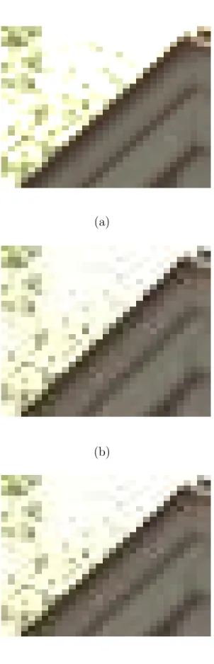
Figure 2.2: PSNR-vs-CR performance of the ‘24’ image from the Kodak dataset for fixed color transforms and the color weight method. (a) Original Image, (b) Rate-Distortion curve. Our method outperforms the baseline transforms. Figure reproduced from Reference [1] with permission.
In Figures 2.2 - 2.2 the rate-distortion curves for ‘24’, ‘23’, ‘Serous-02’ and ‘Lenna’ are given. While v24’, ‘Serous 2’ and ‘Lenna’ are images where our method outperforms the baseline transforms, in image ‘23’ this is not the case.
(a) 6 8 10 12 14 16 18 35 35.5 36 36.5 37 37.5 38 38.5 39 39.5 40 PSNR [dB] Compression Ratio YCbCr Our YCbCr Y‘CbCr Our Y‘CbCr YUV Our YUV (b)
Figure 2.3: PSNR-vs-CR performance of the ‘23’ image from the Kodak dataset for fixed color transforms and the color weight method. (a) Original Image, (b) Rate-Distortion curve. The baseline transforms outperform our method. Figure reproduced from Reference [1] with permission.
(a) 10 15 20 25 32 32.5 33 33.5 34 34.5 PSNR [dB] Compression Ratio YCbCr Our YCbCr Y‘CbCr Our Y‘CbCr YUV Our YUV (b)
Figure 2.4: PSNR-vs-CR performance of the ‘Lenna’ image for fixed color trans-forms and the color weight method. (a) Original Image, (b) Rate-Distortion curve. Our method outperforms the baseline transforms. Figure reproduced from Reference [1] with permission.
(a) 3 3.5 4 4.5 5 5.5 6 6.5 7 32 32.5 33 33.5 34 34.5 35 PSNR CR YCbCr Our YCbCr Y‘CbCr Our Y‘CbCr YUV Our YUV (b)
Figure 2.5: PSNR-vs-CR performance of the ‘01122182-0033-rgb’ image (second image in microscopic image dataset) for fixed color transforms and the color weight method. (a) Original Image, (b) Rate-Distortion curve. Our method outperforms the baseline transforms. Figure reproduced from Reference [1] with permission.
(a)
(b)
(c)
Figure 2.6: A visual result of image ‘24’ from the Kodak dataset coded by JPEG using a quality factor of 80%. (a) Original, (b) JPEG coded version using Y’CbCr and (c) JPEG coded version using the color weight method with Y’CbCr. Figure reproduced from Reference [1] with permission.