A new method for the steady-state analysis of periodically excited nonlinear circuits

964 IEEE TRANSACTIONS ON CIRCUITS AND SYSTEMS-I: FUNDAMENTAL THEORY AND APPLICATIONS, VOL. 43, NO. 12, DECEMBER 1996

A New Metho

Periodically Excited Nonline

Mustafa Celik, Abdullah Atalar, Senior Member, IEEE, and Mehmet A. Tan, Senior Member, IEEE

Abstract- We propose a new method for the steady state analysis of periodically excited nonlinear microwave circuits. It is a modified and more efficient form of Newton-Raphson iteration based harmonic balance (HB) technique. It solves the convergence problems of the HB technique at high drive levels. The proposed method makes use of the parametric dependence of the circuit responses on the excitation level. It first computes the derivatives of the complex amplitudes of the harmonics with respect to the excitation level efficiently and then finds the Pad6 approximants for the amplitudes of the harmonics using these derivatives.

I. INTRODUCTION

TEADY-STATE ANALYSIS methods for nonlinear mi- crowave circuits are classified into three categories ac- cording to the domain in which linear and nonlinear elements are calculated. These are pure time-domain methods [1]-[4], pure frequency-domain methods [ 5 ] , [6], and hybrid time- domaidfrequency-domain methods.

Among these categories, the hybrid frequency-domaidtime- domain technique is accepted to be the most suitable one for the analysis of nonlinear microwave circuits. This technique, which is referred to as harmonic balance (HB) [7], combines the efficiency of frequency-domain analysis of linear circuit elements and the accurate time-domain analysis of nonlin- ear devices. A comprehensive survey of harmonic balance technique can be found in [SI-[12].

From a mathematical point of view, the harmonic balance method converts the problem of solving a set of nonlinear differential equations into the problem of solving a set of nonlinear algebraic equations. The latter is more preferable because it is simpler to solve than the other. The solu- tion of the nonlinear algebraic system is usually obtained by means of a suitable iterative procedure. Therefore, it is clear that the strength of the HB method is determined by the iteration process used. The most common iteration processes are variable metric (quasi-Newton) [SI, relaxation

[ 131, reflection [14], continuation [ 151, and Newton-Raphson [SI techniques. Among these, the Newton-Raphson method is

Manuscript received July 1, 1994; revised July 8, 1995. This work was supported by NATO-SFS project (TU-MIMIC). This paper was recommended by Associate Editor A. Premoli.

M. Celik was with the Department of Electrical and Electronics Engineer- ing, Bilkent University, 06533 Bilkent, Ankara, Turkey. He is now with the Department of Electrical and Computer Engineering, Camegie Mellon University, Pittsburgh, PA 15213 USA.

A. Atalar is with the Department of Electrical and Electronics Engineering, Bilkent University, 06533 Bilkent, Ankara, Turkey.

M. A. Tan was with the Department of Electrical and Electronics Engi- neering, Bilkent University, 06533 Bilkent, Ankara, Turkey. He is now with Silicon Systems Inc., A Texas Instruments Company, Tustin, CA 92680 USA.

Publisher Item Identifier S 1057-7 122(96)08336-5.

known to be the most general and efficient iteration technique. However, like all other locally convergent methods, it has convergence problems. Convergence can be achieved only by finding sufficiently close initial values to the solution, which is difficult particularly for the cases of high excitation levels. This paper describes a new method to obtain the steady-state solution of a nonlinear circuit with periodical excitation. It is a modified form of HB technique based on Newton-Raphson iteration and uses far fewer Newton-Raphson iterations than the HB method. It also solves the convergence problems of the HB technique at high drive levels. The proposed method makes use of the parametric dependence of the circuit re- sponses on the excitation level. It first computes the derivatives of the phasors of the harmonics with respect to excitation level efficiently, and then finds the Pad6 approximants for the phasors of the harmonics using these derivatives. This approximation is valid for a wide range of excitation levels. When the error of approximation grows, a correction is made using a Newton-Raphson iteration by using the last result as the seed.

In Section 11, the method of harmonic balance is revisited and the Newton-Raphson technique is reviewed. Then, in Section I11 we present our method. Section IV presents some examples that show the advantage of the proposed method over the Newton-Raphson technique.

11. THE HARMONIC BALANCE APPROACH Consider a circuit which contains nonlinear elements, linear lumped components, and linear elements specified with fre- quency domain parameters. All nonlinear devices in the circuit will be assumed to be represented by algebraic equations. Let us suppose that the circuit is partitioned into linear and nonlinear subcircuits and let N be the number of ports between these subcircuits. The linear part of the circuit, therefore, is reduced to a N port network which is characterized by a N by N Y-parameter matrix r ( j w ) . Kirchoff s current law requires the following set of nonlinear equations for the port voltages to be satisfied

where y ( t ) is the inverse Fourier transform of T ( j w ) , and v(t) is a vector containing the port voltage waveforms, i,(t) is a vector containing the Norton equivalent source waveforms,

i(v) and q(v) are the functions describing the nonlinear conductances and capacitances in the circuit, respectively. 1057-7122/96$05.00 0 1996 IEEE

CELIK et al.: STEADY-STATE ANALYSIS 965

Let WO be the fundamental angular frequency and H be the highest harmonic number that is taken into account. Therefore, any waveform in the circuit can be approximated with a finite Fourier series

where K z , k is used to represent the phasor for the kth harmonic of the voltage at port i . The above relation can be also represented in the vector notation as a Fourier series pair

v(t)

++

v

(3)

where V = [ V ~ , - H * * . V ~ , O * . * Vl,H"'VN,-H"'VN,O'" VN,HIT. similarly we have, q ( t ) H Q , i ( t ) H I , and

i,(t)

H

I , . Then, (1) can be written in the form [8],

F ( V ) = I ( V )

+

jRQ(V)

+

YV + I , = 0 (4) where F ( V ) is called as the current-error vector and the harmonic balance error is defined as the Z2 norm of the current-error vector

E = II~(V)ll2. ( 5 )

In (4), the admittance matrix Y has the form

y11 " ' Y 1 N

(6) Y N I

...

Y N N

where the submatrices are equivalent to

Yij = diag[Tij(jkwo)], k = - H , . .

.

,

0,

. . .

,

H ₍₇₎ and finally R is a diagonal matrix such that it has N cycles of (-Hwo, e

-

,

0,

-

a

,

Hwo) along its main diagonal.

A. Newton-Raphson Method updated as follows:

In the Newton-Raphson (NR) method, the phasor vector is

Vn+' = V"

-

J(V")-lF(V") (8)

where J is the Jacobian of F ,

(9) In the above equation

and the entries of the submatrices A,, are equivalent to exp(-j(k - l ) w o t ) d t

It is widely known that the NR method is both locally and superlinearly convergent, that is, it is very fast if the starting point is close enough to the final solution, but if the converse holds it may diverge. The time consuming part of the NR method is the evaluation and the inversion of the Jacobian matrix J because of its dense structure. One way to accelerate the NR technique is Shamanskii method, that is, to reuse the inverted Jacobian matrix until the harmonic balance error begins to rise. In another approach, the small terms far from the diagonal in the Jacobian are set to zero, therefore its density is reduced and sparse matrix techniques can be applied. The above approaches are attractive in terms of speed and memory considerations, however, they are poor in convergence.

In order to improve convergence, one can make use of source stepping concept [ 141. This method approaches the desired input level incrementally. The results of a calculation at one level can be used as a good initial estimate for the next level. However, in order to obtain a starting point lying in the region of convergence, the step sizes may have to be very small.

Another technique that can be used to improve the conver- gence is the continuation method. Let us consider a system of nonlinear equations given in the form, F ( X ) = 0. In the continuation method, the problem is replaced by an auxiliary one of the form:

F ( X , p ) = 0 (12) where p is called the continuation parameter. Assuming that a solution X o is known for a certain value of the continuation parameter, e.g., p = 0, this method generates the solution

X

for the desired value of the parameter p by a step-by-step mechanism. In case of electrical circuits, the intensities of the RF sources are taken as the continuation parameter. Therefore,

X o is the result of the dc analysis. Starting from this result, the solution at the desired power level is obtained through a sequence of intermediate solutions corresponding to the increasing values of p. At each intermediate step the nonlinear problem is very well conditioned because the corresponding value of p can be made sufficiently close to the that of previous solution.

Convergence of the iterative techniques can be improved using the continuation method. However, since it uses a first order approximation, the number of intermediate steps in the continuation method can be large and therefore very long analysis time may be required.

111. PROPOSED METHOD

In the following, we propose an extension to the continua- tion method. Unlike the continuation method, our technique uses higher order approximations, and is faster than the conventional HB algorithms. We start by splitting the source vector i s ( t ) into two parts as follows:

i , ( t , p ) = Pi,l(t)

+

i s 2 ( t ) (13) where p is a parameter similar to the one used in the continu- ation method. In our method, the parameter p may be used in many different ways. For instance, in a practical case, i s l ( t ) (11)

The entries of the matrix dQ/aV are similar to those of

966 IEEE TRANSACTIONS ON CIRCUITS AND SYSTEMS-I: FUNDAMENTAL THEORY AND APPLICATIONS, VOL. 43, NO. 12, DECEMBER 1996

dq - _- -

d V

may contain all the RF sources while i s 2 ( t ) contains only dc sources. In another case, i s l ( t ) may contain only one of the sources (RF or dc). Moreover, the parameter p can be used either artificially or naturally in the sense explained as follows. Using p artificially refers to the case where the sources in the vector i s l ( t ) are represented by their actual values and the solution that corresponds to p = 1 is attempted to obtain. It can be also used naturally, that is,

i,l(t)

contains only one source whose value is unity and the parameter p is equivalent to the input excitation level. In this case, a solution as a function of the input level is sought.

Having split the sources as in (13), assuming that all port voltages are continuous functions of the parameter p, we express them in the Taylor series expansion form about a particular value of p as follows:

- &ll(t) %l(t) - dv1 ( t ) dviv ( t )

asN

( t ) &IN ( t ) ~

. . .

~ (20) ~

. . .

~

-

dv1

( t )

a v N ( t )

-

Let V" be the phasor equivalent of the nth order derivatives of the time waveforms, i.e.,

Then we have 00 ( P

-

Po)" n.! ' V ( p ) =

CV".

n=O

The aim of this work is to find good approximations for the nonlinear dependencies of the Fourier coefficients on the parameter p. For this purpose, we first compute the derivatives of the Fourier coefficients with respect to the parameter p , then using these derivatives we find a rational polynomial function of p for each coefficient.

A. Computation of the Derivatives

Using (13) we can rewrite (1) as follows: Y ( t -

447,

P ) d7

+

w ,

P I )

and let us suppose that the solution of (1) is known at p = po.

Then V o = V ( p 0 ) . Now, if we take the derivative of (17) with respect to p and evaluate at p = p o we obtain

k=-H

and let the vectors I and V contain the Fourier series coef-

ficients, i . e . , I =

[I-H,...,IH]~

a n d V =

[V-H,...,VH]~.

Similarly, H g ( t ) = G k e x P ( j k w o t ) (25) k=-H and H c ( t ) = CI,exp(jkwot). (26) k=-H

Then, the time domain input output relations given in (21) and (22) can be represented in the frequency domain as

I = G V (27)

I

=jacv

(28)

where the conversion matrices G and C axe given as [ G o G-l . . . G - - 2 ~ 1

and

= diag[kwo], k = - H , , 0 ,

. . .

H . (31) 'Actually, we have n(t) = C , g , ( t ) v z ( t ) and s(t) = ( d / d t ) ( C , c z ( t ) v z ( t ) ) . However, for simplicity we assume that they are in the form (21) and (22).

CELIK et al.: STEADY-STATE ANALYSIS 967

Applying the conversion matrix techniques to (18) we can

(32)

C. Approximating the Fourier Coeficients

Let

v,

be the phaSOr of the kth harmonic of a port voltage of the circuit and consider its Taylor series expansion about po obtain a set of linear equations for the first order derivative

( Y + A + j R B ) . V 1 = - I s l

where Y is again in the form of (6), but this time its submatrices are the conversion matrices of the corresponding linear elements,

Yij = diag[Tij(jkwo)], k = - H , 1 1

,

0,

. . .

,

H (33)

and the matrices A and B contain the submatrices which are the conversion matrices of the time-varying elements,

[Amn]kl = / T o ' 2

ai,(t)

exp(-j(k - Z)wot) d t . (34) TO - T 0 / 2

T o / 2

exp(-j(k - Z)wot) d t . (35) [Bmnlkl = 1 T 0 / 2

av,(t)

such that IC = - H , e a . , 0 , a . e

,

H and 1 = - H , 0 * , 0 , e a,H

and finally

R

is a diagonal matrix such that it has N cycles of ( -Hwo,

. . .

,

0 , W O ,

.

.

*

,

Hwo) along its main diagonal. A

closer look reveals that the matrix (Y

+

A

+

j R B ) is in fact the Jacobian J .

Similarly, taking the derivatives of (17) repeatedly with respect to p, one obtains (18) with a different excitation vector

(36) where

i"(t)'s

are the sources corresponding to the constants appearing as the result of derivative operations performed on the constitutive relations of the nonlinear elements. Therefore, higher order derivatives can be obtained by solving the same linear equation set with different source vectors

J . V " = -I", n 2 2 (37)

where I" is the phasor equivalent of the waveform

i"(t).

Once the LU factorization of the Jacobian matrix J has been obtained, each derivative can be obtained efficiently only by one forward and one back substitution.

B.. Computation of the Source Vectors

The nth-order excitation vector,

in(t),

is a function of vZ(t)'s, i = l , . . . , n - 1, and derivatives of i(v) and q(v)

with respect to v evaluated at v(t) = v(t, po) up to order n. It is cumbersome to represent the recursive dependence of in

( t )

to the lower order outputs in the matrix notation used above. The procedure for computing the excitation at the nth-order circuit can be best explained at element level. This procedure is called the method of nonlinear currents and the details can be found in [ 5 ] . In the proposed method the symbolic expressions for derivatives are generated only once and embedded into the simulator. During the analysis they are only numerically evaluated and the corresponding computational overhead is very small compared the LU factorization of the Jacobian matrix J as will be demonstrated in Section IV.

00

n=O

where m, = V,'")/n!. If p is very close to po i.e., Ip-po(

<<

1, above series converges rapidly. It is sufficient to calculate only the first few terms. This is also true for weakly nonlinear circuits where the coefficients m, 's decay rapidly. Both cases correspond to the Volterra series analysis when the expansion is performed about p = 0.

For the general case, however, the series given in (38) may be slowly convergent. One can use Pad6 approximation [16], to find an approximation to the exact solution V j ( p ) . Pad6 approximation is preferred over a power series approximation because of its good convergence properties. The objective of Pad6 approximation is to construct a rational function

(39) i=O

such that its Taylor series expansion about po has the same first 2q

+

1 coefficients as that of V, given in (38). The coefficients of the rational functions, therefore, should satisfy

a M

__

n

az(p - Po)z =

Cmz(P

-

POY *

2

bZ(P - P o ) % . (40)

a=O 2=o a=O

Equating the coefficients of the terms of the same degree yields the following systems of linear equations for the coefficients:

bo =mo

bl = moa1

+

ml

and

After the ai's have been obtained from (42), the bi's can be found from (41) by substitution. Since the matrix in (42) is a Toeplitz matrix, an efficient solution is available at the complexity of O ( q 2 ) [171.

The approximation obtained for a particular p is valid in its neighborhood. When the harmonic balance error grows, a correction becomes necessary. For this purpose, a Newton- Raphson iteration may be used by using the last result as an initial guess. A similar approach using power series ap- proximation has been proposed earlier [18]. We use Pad6 approximation instead, because it provides a much larger range of validity.

968 IEEE TRANSACTIONS ON CIRCUITS AND SYSTEMS-I: FUNDAMENTAL THEORY AND APPLICATIONS, VOL. 43, NO. 12, DECEMBER 1996

D. The Algorithm

We can summarize our algorithm as follows.

1) Set p = po (generally po = 0) and find the solution of the circuit using a Newton-Raphson iteration.

2) Applying (37) compute the derivatives of the Fourier coefficients. Then performing Pad6 approximation for each coefficient, obtain the estimated solution V ( p ) . 3 ) Increase p until the harmonic balance error, as defined

in (5), becomes larger than a predefined tolerance, €1. Then, at that particular value of p , find the solution using Newton-Raphson method with last result as a seed (i.e., decrease the HB error to another tolerance €2 ( € 2

<

€1)).

Go to step 2.

Iv. RESULTS

The algorithm proposed in this paper is not a completely new analysis technique, but a modified form of Newton- Raphson based harmonic balance technique and it may be adopted in existing harmonic balance simulators to reduce the number of iterations drastically. Therefore, we prefer the following method for performance comparison, which we believe is a fair one. To count the number of iterations required for our method, we used a commercial simulator: Microwave Harmonica from Compact Software [19]. In Mi- crowave Harmonica, one can provide initial solution estimate to the simulator using the xxx.vcIr file. The simulator reads this file and starts Newton Raphson iterations from this initial guess. All the iterations reported in the paper are carried out by Microwave Harmonica and we believe that the iteration comparison (whether they are Shamanskii or actual Newton- Raphson) in this way is homogeneous. Moreover, the simulator is more likely to use Shamanskii iteration in our case because our initial estimates are already very close to the actual solution.

In order to demonstrate the efficiency of the proposed method we examine some example circuits.

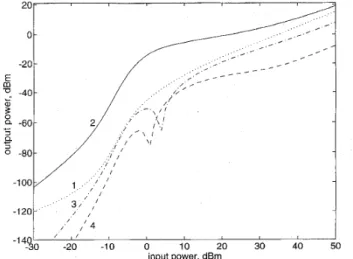
Example 1: We first consider a doubler circuit whose schematic is shown in Fig. 1. The diode in the circuit has the following characteristics:

(43) where I , = l e

-

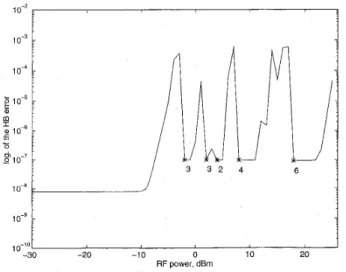
06 and V, = 1/35. This circuit was analyzed as a function of input excitation level, using the method proposed in this paper. The first four harmonics of the load voltage are plotted in Fig. 2. The HB error is shown in Fig. 3 as a function of the input power. In the same figure, the stars indicate the points where a Newton-Raphson iteration is needed, and the numbers below them indicate how many such iterations are performed. In the small-signal region, our method and the Volterra series approach performs similarly. As p is growing, the error increases. When the error exceeds € 1 = Newton-Raphson iterations are performed

to reduce the error below €2 = lop7. The approximation obtained from the new solution is valid in about 10 dB range. In Fig. 4, our method is compared with Microwave Harmonica in terms of number of Newton-Raphson iterations. The circuit was analyzed with 2 dB increments in Microwave Harmonica,

I = Is[exp(V/K) - I]

R1 I=f(V)

Fig. 1. Doubler circuit (R1 = 830, C1 = 0.1592F, L1 = 0.1592H, R2 = 1R, C2 = 0.0796F, L2 = 0.0796H, R3 = 5 9 0 )

I

I ' ,/'4

I

, ,

- 1 4 . d ~

-io

-,o

A

10

io io

40

A

input power, dBm

Fig. 2. Powers of the harmonics at the load (doubler circuit)

-*/

-4t

i

-16 -I4[

:I

-l8IJ

1

-20 - 7 0 0 I O 20

3b

4'0 20 input power, dBm

Fig. 3. Harmonic balance error versus input power (el = l O W 5 , e 2 = l o p 7 ) (doubler circuit).

where the error limit was set to In order to obtain the response of the circuit for an input power range from -30 to f50 dBm, Microwave Harmonica needs a total of 300 Newton-Raphson iterations while our method finds the same result with only 20 iterations.

In Figs. 5, 6, and 7, we compare the performance of the Pad6 approximation with the Taylor series approximation for the dc component, the first harmonic and the eighth harmonic of the voltage waveform on the diode of the doubler circuit. Using the solution of the circuit at V,, = 4 V, we computed the first 16 derivatives of the Fourier coefficients. As seen from

CELIK et al.: STEADY-STATE ANALYSIS or!

5

i o 15 io 5;

io

35 ‘lo 969 45 141 I I 12- U) B 10- E

-

._ * Microwave Harmonica 0 proposed method 36% * * * * * * * x x * * * * x x * x * - x x * * * * x (1 0 0 1 6 - 0016- 2 0.014 E l 20012: $ 0.01 ;0008+ L B I I 0 1 e ’ 5 1 $0006+ 0004; 0 -

;

I

,

0 $0 -20 .IO 0 I O 20 30 40 input power, dBm Fig. 4. cuit).

Comparison of number of Newton-Raphson iterations (doubler cir-

_ _ _ Pade approx.

oov

5

Ib

15 40 ;5

i o

i5 ‘lo

b

I

excitation level (volts)

Fig. 5.

nent (doubler circuit).

Comparison of Pad6 and polynomial approximations for dc compo-

the figures, the @/SI Pad6 approximations of the dc component and first harmonic remain valid up to V;, = 40 V, while the fifteenth-order Taylor series approximation is valid only up to V;, = 8 V. For higher harmonics the region of accuracy is smaller compared the lower harmonics due to smaller accuracy in higher harmonics, but as shown in Fig. 7, the approximation of the eighth harmonic (highest harmonic) is still valid for a very broad range (up to V;, = 30 V).

Example 2: The second example is a GaAs MESFET cir- cuit whose nonlinear equivalent circuit is shown in Fig. 8. The following relation was used for drain current [14]:

Id = (A0

+

AlV,

+

A2V;

+

&V’) tanh(aVd) (44) where A0 = 0.5304,Al = 0.2595,A2 = -0.0542,A3 = -0.0305, and a = 1. Using the proposed method, we analyzed the circuit as a function of the input power level. We used [7/8] Pad6 approximations and we chose c1 =

First, we found the dc operating points by setting the RF drive level to zero. Then, we obtained an approximation about

and €2 = 0. - Exact Polynomial approx. Pade approx. _ - _ 0.02, _I

o.oo2/,

1

Pade approx.

- _

0;

’

;

;1 15 io ;5

io

3; 40 a5

I

excitation level (volts)

Fig. 7.

tude of the eighth harmonic (doubler circuit).

Comparison of Pad6 and polynomial approximations for the ampli-

zero excitation level which is valid up to +32 dBm. The new approximation found at +32 dBm remains accurate up to +36 dBm. We used only 10 Newton-Raphson iterations. However, Microwave Harmonica needs approximately 150 Newton- Raphson iterations to find the response of the circuit from 0 dBm to $36 dBm with 1

dB

increments. First three harmonics of the load voltage are plotted in Fig. 9. Fig. 10 shows how the HB error is changed during the analysis procedure in our method. Again the stars indicate the points where a Newton- Raphson iteration is needed, and the numbers below them indicate how many iterations have been performed.

Example 3: The next example is a doubly balanced diode mixer circuit shown in Fig. 11. It is taken from Microwave

Harmonica manual. The diodes are identical and have the characteristics given in (43). The circuit is chosen as an exam- ple in the manual, because it has convergence problems when only Newton-Raphson iteration is used and it is suggested to analyze the circuit with 10 quasi-Newton and convergence factor of 0.5. We chose the RF and LO frequencies as 3 and 2 Hz, respectively, and analyzed the circuit using the proposed

970 IEEE TRANSACTIONS ON CIRCUITS AND SYSTEMS-I: FUNDAMENTAL THEORY AND APPLICATIONS, VOL. 43, NO. 12, DECEMBER 1996 E B -10- 0 g-20-

-

_m 5 -30- -40 -50 -60

Fig. 8. Mesfet circuit (Vbl = -O.SV,Vb, = 12V, Rgen = R1 = 50R,

Lb 1OOOH, Cb = IOOOF, R, = 10, R, = 0.7R, Cds = 0.006F, Cd = O.O02F, C , = 0.03F) > - 2 - ,' 3 - - 1 ' I

Fig. 10. Harmonic balance error versus input power (€1 =

€ 1 = IO-*) (mesfet circuit).

method for a LO power level of 20 dBm and a RF power range from -30 to +25 dBm. The magnitudes of the various harmonics at the IF port are shown in Fig. 12. In Fig. 13, the HB error is plotted. Our method needs only 18 iterations provided that the solution for +20 dBm LO and zero RF level is known. To find the solution for that case, our method needs additional three corrections with 13 iterations. On the other

1:11

c';7

6R

Fig. 11. Doubly balanced diode mixer circuit.

, , -45

[,

, , , ' -50 ,'

I

I ' I -30 -20 -10 0 10 20 RF power, dBm

Fig. 12. Powers of the harmonics at the IF port (mixer circuit)

I 0.' J

i

I -20 -10 0 10 20 1 0 - ~ 0 ~ -30 RF power, dBm

Fig. 13. Harmonic balance error versus input power (€1 = l o w 4 ,

€1 = l o p 8 ) (mixer circuit).

hand, Microwave Harmonica needs thousands of iterations (3 1 quasi-Newton and 6905 Newton-Raphson iterations) to find the response for

RF

power range from -30 dBm to +25 dBm with 1

dB

increments.

CELIK et al.: STEADY-STATE ANALYSIS 97 1

The example above also demonstrates how the proposed method helps convergence. To find the solution for 20 dBm LO and zero RF level, Microwave Harmonica needs 36 quasi- Newton and 25 Newton-Raphson iterations. Our method solves this problem by using 13 Newton-Raphson iterations without requiring any quasi-Newton iterations. quasi-Newton is a more robust but slower method that is used in some HB simulators when NR technique fails to converge. This example shows that our method is more efficient than the conventional techniques, even at single level analysis. For power sweep applications, however, the proposed method becomes much more efficient as the above three examples illustrate.

Our algorithm introduces a computational overhead mainly due to the evaluation of derivatives and Pad6 approxima- tion. Determination of this overhead is necessary for a fair assessment of our algorithm. Unfortunately, a direct CPU time comparison is not possible since we did not have an access to the FORTRAN source code and were unable to integrate our algorithm into the commercial package. Instead, this part of the computation was programmed using MATLAB [20]. MATLAB reports the computational burden in mflop (mega floating point operations) units. Experiments indicate that a MATLAB (an interpreter rather than a compiler) code containing many loops will run 10 to 20 times slower than a FORTRAN counterpart in the same machine. Using above figures and mflop/s rating of the SPARC 2 machine we estimate that computational overhead is equivalent to one to two iterations. For example, double balanced mixer circuit requires 2.5 mflop for the derivative computation in one expansion point. With a machine with 5 mflop/s peak rating, this computation can be done in 0.5 to 1 s using FORTRAN or C. (MATLAB on the same machine calculates the same 2.5 mflop in 11.5 s, consistent with the slowdown figures above). On the other hand, one Microwave Harmonica iteration on the same machine takes about 0.5 s. Therefore, the computational overhead is approximately equivalent to one or two iterations. Hence, for a fair comparison we should increase the number of iterations at each correction point by one or two. Even so, our algorithm introduces a significant improvement over the conventional HB algorithm.

V. CONCLUSIONS

In this work, we have proposed a new method for the steady- state analysis of nonlinear microwave circuits. Our method has mainly three advantages over the conventional HB method: i) it finds a parametric solution with respect to the input power level; ii) it is much more efficient than the HB method in terms of number of Newton-Raphson iterations; iii) it provides faster convergence compared to the HB method.

This paper has presented examples to illustrate the efficiency

of the proposed method over the conventional HB method. For this purpose, we have used the commercial simulator Microwave Harmonica (version 2.0) and observed that the required number of NR iterations reduces drastically when the proposed method is used. We have to note that version 2.0 is not the latest release of the software. The latest releases of the HB simulators make use of all recently proposed techniques

and are more efficient compared the previous ones. Had one of these modern simulators been used instead of old version we used in our experiments, the reduction in the number of NR iterations would not have been so dramatic. However, we are confident that our method can improve the efficiency of these new simulators even further.

ACKNOWLEDGMENT

The authors would like to thank M. Ozgur for his help. The reviewers are also acknowledged for their very valuable comments.

REFERENCES

[l] L. W. Nagel, “SPICE2: A computer program to simulate semiconductor circuits,” Tech. Rep. Memo ERL-M520, Univ. Calif., Berkeley, May 1975.

[2] T. J. Aprille and T. N. Trick, “Steady-state analysis of nonlinear circuits with periodic inputs,” Proc. IEEE, vol. 60, pp. 108-114, Jan. 1972.

[3] F. R. Colon and T. N. Trick, “Fast periodic steady-state analysis for large signal electronic circuits,” IEEE J. Solid-State Circuits, vol. SC-8,

pp. 260-269, Aug. 1973.

[4] S. Skelboe, “Computation of the periodic steady-state response of nonlinear networks by extrapolation methods,” ZEEE Trans. Circuits [5] S. L. Bussgang, L. Ehrman, and J. W. Graham, “Analysis of nonlinear systems with multiple inputs,” Pmc. IEEE, vol. 62, pp. 1088-1 119,

Aug. 1974.

[6] G. W. Rhyne, M. B. Steer, and B. D. Bates, “Frequency-domain non- linear analysis using generalized power series,” IEEE Trans. Micmwave Theory Tech., vol. 36, pp. 379-387, Feb. 1988.

[7] M. S. Nakhla and J. Vlach, “A piecewise harmonic balance technique for determination of the periodic response of nonlinear systems,” IEEE

Trans. Circuits Syst., vol. CAS-23, pp. 85-91, 1976.

[SI K. S. Kundert and A. Sangiovanni-Vicentelli, “Simulation of nonlinear circuits in the frequency domain,” IEEE Trans. Computer-Aided Design,

[9] V. Rizzoli and A. Neri, “State of the art and present trends in nonlinear microwave CAD techniques,” IEEE Trans. Microwave Theory Tech.,

vol. 36, pp. 343-365, Feb. 1988.

[lo] R. J. Gilmore and M. B. Steer, “Nonlinear circuit analysis using the method harmonic balance-A review of the art. Part 1. Introductory concepts,” Int. J. Micmwave Millimeter- Wave Computer-Aided Eng., SyStS., vol. CAS-27, pp. 161-175, Mar. 1980.

vol. CAD-5, pp. 521-535, Oct. 1986.

VOI.

1,

pp. 22-37, 1991.

1111 ~, “Nonlinear circuit analysis using the method harmonic bal- -

-ance-A review of the art. P& 2. Advanced concepts,” Int. J. Mi- crowave Millimeter-Wave Computer-Aided Eng., vol. l , pp. 159-180, 1991.

[12] V. Rizzoli, A. Lipparini, A. Costanzo, F. Mastri, C. Cechetti, A. Neri, and D. Masotti, “State of the art harmonic balance simulation of forced nonlinear microwave circuits by the piecewise technique,” IEEE Trans. Micmwave Theory Tech., vol. 40, pp. 12-28, Jan. 1992.

131 R. G. Hicks and P. J. Khan, “Numerical analysis of nonlinear solid- state device excitation in microwave circuits,” IEEE Trans. Microwave Theory Tech., vol. MTT-30, pp. 251-259, Mar. 1982.

141 S. Mass, Nonlinear Microwave Circuits. Nonvood, M A Artech House, 1988.

151 D. Hente and R. H. Jansen, “Frequency domain continuation method for the analysis and stability investigation of nonlinear microwave circuits,”

IEE Proc., vol. 133, Oct. 1986.

161 G. A. Baker, Essentials of Pad6 Approximants. New York: Academic, 1975.

[17] M. H. Press, €3. P. Flannery, S . A. Teukolsky, and W. T. Vetterling,

Numerical Recipes in C. Cambridge, U.K.: Cambridge Univ. Press,

1988.

[18] E. V. D. Eijnde and J. Schoukens, “Steady-state analysis of a period- ically excited nonlinear systems,” IEEE Trans. Circuits Syst., vol. 37,

pp. 232-242, 1990.

[ 191 MICROWAVE HARMONICA, Compact Software Inc., Patterson, NJ,

User’s Guide.

972 IEEE TRANSACTIONS ON CIRCUITS AND SYSTEMS-I: FUNDAMENTAL THEORY AND APPLICATIONS, VOL. 43, NO. 12, DECEMBER 1996

Mustafa Celik was bom in Konya, Turkey, in 1966. He received the B.S. degree from the Middle East Technical University, Ankara, Turkey, in 1988, and the M.S. and Ph.D. degrees from Bilkent University, Ankara, Turkey, in 1991 and 1994, respectively, all in electrical engineering.

From 1994 to 1996, he was with the Department of Electrical and Computer Engineering, University of Arizona. Currently, he is a research associate with the Department of Electrical and Computer En- gineering, Carnegie Mellon University, Pittsburgh,

Mehmet A. Tan (SM'94) was born in 1959 in Adana, Turkey. He received the B.S. and M.S. degrees both in electrical engineering from Istanbul Teknik Universitesi, Istanbul, Turkey, in 1980 and 1982, respectively, and the Ph.D. degree, also in electrical engineering, from the University of Min- nesota, Minneapolis, in 1988.

He was Associate Professor of Electrical Engi- neering with the Department of Electrical and Elec- tronics Engineering, Bilkent University, Ankara, Turkey, from 1988 to October 1995. He is now with PA His research interests include circuit, interconnect, and mixed-signal

simulation.

Silicon Systems Inc , A Texas Instruments Company, Tustin, CA. His active research interest includes analog integrated filters and computer-aded analysis of electronic circuits.

Dr Tan served as the Chairman of IEEE Circuits and Systems Society Turkey Chapter from 1992 to 1994, and served as the Chairman of IEEE Turkey Section from 1994 to 1996.

Abdullah Atalar (SM'90) was born in Gaziantep,

Turkey, in 1954. He received the B.S. degree from the Middle East Technical University, Ankara, Turkey, in 1974, the M S and Ph D degrees from Stanford University, Stanford, CA, in 1976 and 1978, respectively, all in electrical engineering. His thesis work was on reflection acoustic microscopy

In 1979 he was with Hewlett Packard Labs, Palo Alto, CA, engaged in photoacoustics research. From 1980 to 1986 he was on the faculty of the Middle East Technical University as an Assistant Professor From 1982 to 1983 he was on leave from the University, and was with Ernst Leitz Wetzlar, West Germany, where he was involved in the development of the commercial acoustic microscope In 1986 he joined the Bilkent University and served as the founding Chairman of the Electrical and Electronics Engineenng Department where he is currently a Professor His current research interests include computer-aided design of VLSI and MMIC circuits, micromachined sensors, and actuators

Dr. Atalar is a member of the Turkish Academy of Sciences He was awarded Science Award or TUBITAK, Turkey in 1994