Keywords: Correlated Demands, Heuristics, Hold-Back, Optimal Transshipments, Sensitivity Studies
1 InTroduCTIon
In a highly competitive business environment, after-sales service quality is crucial to improve the overall experience of existing customers and to boost purchase intentions of new customers (Ranaweera & Neely, 2003). An unexpected disruption to after-sales service can severely undercut the current demand (Zandi, 2008). Besides, service quality is important to
guar-Meeting Correlated Spare
Part demands with optimal
Transshipments
Nagihan Çömez, Bilkent University, Turkey Kathryn E. Stecke, University of Texas at Dallas, USA Metin Çakanyıldırım, University of Texas at Dallas, USA
abSTraCT
This paper studies spare part transshipments between two service part facilities whose demands are correlated. Transshipments are used to reduce severity of part stock outs. Facilities are run by an inventory manager (IM) who minimizes replenishment, transshipment, and inventory costs. We show that the optimal transshipment policy is an inventory hold-back type; if the part inventory at a facility is less than or equal to its hold-back level, a transshipment request made for that part by a stocked out retailer is rejected. The hold-back levels increase toward the next replenishment of partsThis implies that transshipment requests are initially accepted until a critical time and afterwards they are rejected. A heuristic is designed using this critical time as the single decision variable. It performs within 0.7-1.8% of the optimal cost. Heuristic policies of no inventory sharing and complete sharing, respectively, perform within 3% and 2% of the optimal cost. Since the computation of hold-back levels and implementation of the optimal transshipments, respectively, require limited resources and little IM oversight, we advocate for the use of the optimal transshipment policy.
antee the continuity of demand for the service operations, which constitute 40-80% of some manufacturers’ profit (Wu & Tew, 2005). After-sales service can be counter cyclical to original equipment sales. In the four month period starting with the U.S. Senate hearings on dropping automobile sales in December 2008, the stock prices of car part suppliers Autozone, Advanced Auto Parts, and O’Reilly Automotive have, respectively, increased by 60%, 46%, and 52% while the same numbers have been -7% and -58% for Dow Jones Industrial and General
Motors. This indicates a negative correlation between after-sales service demand and original equipment demand. Thus, the significance of after-sales service can increase even further in economic slumps.
Responsiveness of the service is an im-portant dimension of service quality. In many studies, part availability is shown to be a significant determinant of response time and thus the determinant of service quality. Wu and Tew (2005) state that dealer stock outs for service parts lead to either increased costs due to emergency orders or unsatisfactory service for vehicle owners. Shahla (2006) mentions that usually ``users perceive customer service as the availability of an item”.
To improve part availability without in-creasing overall inventory levels, inventory sharing among service facilities is an effective strategy. In an inventory sharing system, a service facility that is stocked-out of a certain part and has a request waiting to be satisfied by using that part may receive the part from another facility. Inventory sharing is commonly practiced to increase part availability either for internal operational use or for after-sales repair services. Sharing of repair parts for construc-tion equipment, aircraft, and power-generating plants are considered in Grahovac and Chakra-varty (2001) and Kukreja, Schmidt, and Miller (2001). Flint (1995) estimates that the airline industry stores $45 billion worth of spare parts and suggests that spare parts inventories can be reduced by developing supplier partnerships that include transshipments.
Inventory sharing in distribution systems, such as Volvo GM Heavy Truck and Okuma America, are flexible and responsive because they leverage opportunities and share capabili-ties (Narus & Anderson, 1996). To concretely visualize and to continue with the earlier auto-mobile example, companies such as Autozone, Advanced Auto Parts, and O’Reilly Automotive are among the application areas of inventory sharing. Finding company-issued reports on lack of inventory sharing is harder as such reports can indicate lack of customer service. However, customers publicly complain (Complaints.com,
2002, 2007a, b, c) when the inventory is not shared to meet their demand.
The common features of a repair part often include significant replenishment times from manufacturers and fairly high profit margins. Another feature is low and infrequent demand for the part because of its specific functionality and/or high variety within its product family. Orders for low-demand products usually ar-rive in single-units and monthly demand is often in two digits, e.g., around 25 for a spare part (Zhao, Deshpande, & Ryan, 2005). For these, a low level of inventory can be kept at each facility by relying on inventory sharing to handle stock-outs.
In this paper, we study a centralized system of two service facilities, which are replenished periodically by a manufacturer for a single part type. Between two replenishments, a stocked-out facility (requesting facility) can request a part from another facility (requested facility). The requests are accepted/rejected by an Inven-tory Manager (IM) in charge of the centralized system. If the request is accepted, the requested facility sends the part to the requesting facility. The part takes a transshipment time to arrive at the requesting facility. If the request is rejected, satisfaction of customer service is delayed until the next replenishment. During both the trans-shipment time and waiting time until the next replenishment, backorder cost per unit time is charged. Taking both the transportation time and cost between locations into account, we strive for a realistic model of inventory sharing, called transshipment.
The time between two replenishments in a row is called the replenishment cycle. The IM decides on the order quantities at the beginning of the replenishment cycle and transshipments during the cycle to minimize the system cost including inventory holding, backorder, trans-shipment, and ordering costs. With this objec-tive, we obtain an optimal transshipment policy that is specified by facility-specific dynamic hold-back levels, which are functions of the number of periods until the next replenishment from the manufacturer. These levels can be communicated to each facility at the beginning
of the cycle to make the IM’s oversight unnec-essary during the cycle and hence to facilitate the implementation.
Here we study transshipments that are allowed after, hence depending on, demand realizations called lateral transshipments, first studied by Krishnan and Rao (1965). Signifi-cant amount of work in this area is devoted to centrally managed systems with the exception of some decentralized systems (Rudi, Kapur, & Pyke, 2001; Anupindi, Bassok, & Zemel, 2001; Zhao et al., 2005; Sošić, 2006; Çömez, Stecke, & Çakanyıldırım, 2009b).
Previous studies mainly focus on replenish-ment policy while transshipreplenish-ments are often considered by preestablished rules. Herer and Rashit (1999) studies the effect of fixed and joint ordering costs. Tagaras and Cohen (1992) and Tagaras (1999) introduce non-zero replen-ishment lead times. In Axsäter (1990), Graho-vac and Chakravarty (2001), and Kukreja et al. (2001), replenishment is made after each de-mand arrival called one-for-one replenishment. Xu, Evers, and Fu (2003) analyze a two-location transshipment model using an ( , )R Q replenish-ment policy under a customer service consid-eration.
Studies considering multiple transship-ments in a replenishment cycle are scarce in the literature, except Archibald, Sassen, and Thomas (1997) and Çömez, Stecke, and Çakanyıldırım (2009a) in a centralized setting and Çömez et al. (2009b) in a decentralized setting. In Archibald et al. (1997), unsatisfied demands are satisfied through emergency orders from the manufacturer, so there is no backorder-ing at the service facilities. Inventory holdbackorder-ing cost is charged only at the end of a replenish-ment cycle but not throughout. The demands are independent Poisson processes. The optimal policy obtained in Archibald et al. (1997) can be shown to imply increasing1 hold-back levels
with the time until the next replenishment. In contrary, Çömez et al. (2009a) show that optimal hold-back levels are decreasing in time when there is non-negligible transshipment time and continuously incurred holding and backorder costs. Namely, facilities in their setting are more
likely to transship inventory at the beginning of a replenishment cycle than those in Archibald et al. (1997). Both policies are optimal for their respective settings. However, the situation is delicate; a practitioner must implement the policy appropriate for his/her setting to avoid doing the opposite of the optimal. We also study a setting similar to that in Çömez et al. (2009a) to study demand correlation and heuristic trans-shipment policies.
Although scarce, there are transshipment studies considering the dependencies between the demands of transshipping facilities. All of these studies investigate replenishment poli-cies while assuming complete pooling (Herer, Tzur, & Yücesan, 2006; Dong & Rudi, 2004; Zhang, 2005). To the best of our knowledge, there is no study of demand dependencies with optimal transshipment policies. Zhao, Ryan, and Deshpande (2008) lists consideration of dependent demands as a future work.
This paper provides optimal and imple-mentable transshipment and replenishment policies by incorporating more aspects of reality than previous studies. These aspects include holding costs incurred within a replenishment cycle, backordering costs, multiple transship-ments within a replenishment cycle, positive transshipment times and costs, and dependent demands. Thus, we provide a realistic spare parts inventory sharing model that can help service facilities to increase their coordination and hence part availability without increasing investment in parts, which are reported among the top ten challenges faced by service part facilities (Boone, Craighead, & Hanna, 2008).
2 TranSShIPMEnT and
rEPlEnIShMEnT ModEl
Before proposing a mathematical model, we discuss the ingredients and setting of the model.
Dependent demands: A demand model is
a good starting point for studying spare parts availability. Spare part demands are known to be erratic and low (Grahovac & Chakravarty, 2001; Kukreja et al., 2001). For a particular
part, there may be extended periods of time with no demand. For example, demands for a spare part of Airbus A320 aircrafts employed by Alitalia are zero for several months (Regattieria, Gamberi, Gamberini, & Manzini, 2005). This sort of demand sparsity can justify adopting a Poisson process for the demand at a single service facility.
Zhang (2007) states that ``when few play-ers compete in a market, their strategic interac-tions are likely to produce demands that are cross-correlated”. To jointly study part avail-ability at several service facilities, a joint de-mand distribution is needed, whose marginal distributions preferably yield Poisson demands. Failing to find such a demand model in the literature, we propose one. We develop a discrete time model by dividing a replenishment cycle into N short decision periods as in Lee and Hersh (1993). By choosing N arbitrarily large, the decision periods can be made short enough to accommodate at most one spare part demand at each facility. For two service facilities, let
p11 be the probability of demand at both fa-cilities 1 and 2, and let p00 be the probability of no demand at either facility. p10 and p01 are the probabilities of a spare part demand only at facility 1 and only at facility 2, respectively, where p00+p01+p10+p11= 1. The correla-tion of demands at these two facilities is
r = ( )( )( )( ), 00 11 01 10 10 11 01 00 01 11 10 00 p p p p p p p p p p p p − + + + + (1) which signifies the versatility of the demand model by allowing negatively, positively cor-related, or independent demands. Method of moments estimators can be used to fit the em-pirical demand data to this model. The details are presented in Appendix A.
Spare part demands at different facilities are positively correlated if these facilities are sub-ject to the same demand drivers. For example,
Çakanyıldırım et al. (2008) note a heat wave as a cause of air conditioner failures and show it to be a major driver of air conditioner demand.
On the other hand, demands can be nega-tively correlated when a random market size is randomly split between two facilities. To illus-trate, think of Camry flat tire replacements by two Toyota service facilities in a city: Northern Toyota is in the north and Southern Toyota is in the south. When there is a Camry with a flat tire, it can be towed to either Northern Toyota or Southern Toyota depending on which is closer and/or which/if a facility covers the replacement under a warranty, etc. Thus, there is a nega-tive correlation between facility demands as a consequence of such a split of the total random tire demand. This example can be replicated for other car service parts such as batteries, brake pads/liquids, and windshields.
A special case of our demand distribution,
p11= 0, yields a multinomial distribution, used as a demand distribution in different contexts by Lee and Tang (1998) and Righter and Shan-thikumar (2001). Each of our marginal distribu-tions converges to a Poisson distribution in the limiting case of N → ∞ when p11= 0, and
Np01 and Np10 are kept constant. Thus, our demand model generalizes the one in Archibald et al. (1997).
In this paper, we study the stocking of the same spare part at two facilities. We can also study stocking two spare parts at the same facil-ity with the same model. We only need to in-terpret pij as the probability of demand of i for part 1 and demand of j for part 2 for
i j, Î{0,1}. This interpretation easily extends to the forthcoming parameters. In that case, a transshipment has to be thought as a spare part substitution, perhaps after a modification cost (analogous to a transshipment cost). This sub-stitution is called cannibalization in Kennedy, Patterson, and Fredendall (2002), which puts forth justification of cannibalization as an important issue often faced by maintenance
managers. Our model weighs the modification cost, holding/backorder costs, and future de-mands to mathematically justify spare part cannibalization.
Kennedy et al. (2002) also underline that ``part failures are often dependent”. For example, consider the fan of a heat sink in a computer. If the fan fails, the temperature rises inside the computer, which in turn damages the sensitive electronic equipment such as the processor. In this case, fan and processor failures are naturally dependent. This dependence leads to dependent demands for spare parts. To the best of our knowledge, there is no dependent demand model for spare parts in the literature.
Multiple transshipments per replenish-ment cycle: In practice, a facility that receives a
customer demand may respond to the customer in several different ways, such as satisfying the demand immediately, promising to provide the item from another facility, or backordering until the next replenishment. However, whatever the response is, the facility should respond to the customer quickly. Therefore, we allow for a transshipment decision after each individual demand realization. Most transshipment stud-ies, except for Archibald et al. (1997), allow a single transshipment either in the middle or at the end of a replenishment cycle. The problem with transshipment in the middle of the cycle is that facilities rarely run out of inventory before the middle of the cycle, so transshipments are often not needed. The problem with transship-ment at the end of the cycle is problematic as well. In that case, a stocked out facility can order from the manufacturer instead of re-questing transshipments from another facility. Restricting transshipments to the middle or the end of a cycle does not allow their use at their full potential. In practice, each customer request should be immediately responded to. The response can involve backordering whose cost should be captured properly. These are important ingredients of our model.
Post-stock-out transshipments: We have
learned through our personal communications with car service facilities of several brands that transshipments happen generally after
stock-outs and not before. Given that spare parts are generally high in variety and thus have low de-mand rates per type (Grahovac & Chakravarty, 2001), transshipments before a stock-out have a high risk of remaining in inventory until the next replenishment. In view of our application of transshipments to slow moving service parts as an emergency source of demand supply, a transshipment before demand materialization is unlikely. Especially when transshipment costs are significant, receiving a transshipment before a stock-out would likely not benefit the system. Furthermore, when the transshipment lead time is short, the issue of transshipping before a demand realization is minor (Grahovac & Chakravarty, 2001; Zhao et al., 2006).
Transshipment lot size of one: Service
facilities usually get the regular replenishments by the supplier’s own fleet and use 3PL for transshipments. The reasons are that transship-ment quantity is much less than replenishtransship-ment quantity and that transshipment times are not predetermined unlike replenishment times. In our model, inventories are transshipped in single units. This follows from practice, where the economies of scale provided by third party carriers are generally not large enough to com-pensate for the expected additional backorder cost of delaying transshipments to consolidate them into a single shipment. Note that the pre-vious studies consider no economies of scale in transshipment cost (Archibald et al., 1997; Zhao et al., 2005, 2006). To avoid delays due to consolidation, a facility can perhaps transship in expectation of the stocked-out demand before it happens. But this violates post-stock-out transshipments explained above.
2.1 System Cost
The replenishment problem is modeled over a horizon of infinitely many replenishment cycles. Within a cycle, V x xn( , )1 2 stands for the mini-mum expected total cost in the remaining n periods until the next spare part replenishment if the current inventory levels are x1 and x2 at facilities 1 and 2. The optimal centralized cost
V x xn( , )1 2 is recursively obtained in three cases: (i) when both facilities have stock; (ii) when both are stocked-out; (iii) when one is stocked-out, while the other still has stock.
Let N = {1,2, } be the set of natural numbers and N-= {0, 1, 2, }- - be the set
of nonpositive integers. In period n , if the current inventory levels of both facilities are positive, each facility satisfies his own demand if it exists. V x xn( , )1 2 is calculated by
condition-ing on the demand arrivals at facilities.
V x xn( , )1 2
x x1, 2Î N , (2)
where hi is the holding cost at facility i . If
both facilities are stocked out, any demand arrived is backordered and a backorder cost until the next replenishment is incurred.
(3) where p is the backorder cost.
In a replenishment cycle, suppose that fa-cility 2 stocks-out before fafa-cility 1. Each time facility 2 needs the part, a request is sent to facility 1. The request is accepted if this results in lower system cost for the remainder of the replenishment cycle; otherwise it is rejected. This tradeoff is captured by minima below.
V x xn( , )1 2
x1≥2,x2 ∈N −, (4)
where K is the transshipment cost. K can include transportation cost as well as holding and backorder costs during a transshipment, which takes a positive amount of time.
A facility meets her own demand before entertaining transshipment requests.
(5) At the end of a cycle, right before a replen-ishment arrival,
V x x0( , ) = 0.1 2 (6)
Since the facilities are arbitrarily numbered, we do not explicitly consider cases obtained by replacing x1 with x2 such that
[x1∈N−,x2= 1], which is analogous to (5). During a replenishment cycle, facilities 1 and 2 face binomial demands denoted by random variables Bin N p( , 10+p11) and
Bin N p( , 01+p11). Facility inventories are replenished based on the demands x1 and x2
handled by facilities 1 and 2. If no facility stocks out, demands x1 and x2 are Bin N p( , 10+p11)
and Bin N p( , 01+p11). On the other hand, a facility that transships to a stocked-out facility handles more demand than the binomial demand she faces from her own customers. In particu-lar, if facility 2 stocks out and facility 1 trans-ships k parts, x1 =Bin N p( , 10+p11)+k and
x2 =Bin N p( , 01+p11)−k . To highlight the dependence of xi on the inventory levels ( , )z z1 2
at the start of a replenishment cycle, its de-noted by xi( , )z z1 2 . Since the total demand met
by the facilities is equal to the total demand arriving into the system, we have , which is independent of the inventories
( , )z z1 2 .
2.2 optimal replenishments
In the replenishment problem, the amount of inventory ( , )z z1 2 to start a replenishment cycle is determined when the inventory level ( , )y y1 2
at the end of the previous cycle is given. After ordering z1-y1 and z2-y2 at a cost of c per item at the beginning of a cycle, the demand is met over a replenishment cycle by incurring the cost V z zN( , )1 2 . The cost over infinitely many replenishment cycles can be calculated by a dynamic program. W y y c z z y y V z z z y z y N ( , ) =1 2 { ( ) ( , ) 1 1,2 2 1 2 1 2 1 2 ≥min≥ + − − + +αE W z[ ( 1−ξ1( , ),z z1 2 z2−ξ2( , )]},z z1 2 (7) where a is the discount factor over a replenish-ment cycle. From (7), it is clear that each re-plenishment problem requires the solution of
the transshipment problem to get V z zN( , )1 2 in
equations (2)-(6). Thus, the transshipment problem is nested within the replenishment problem.
Although (7) appears to be a standard dynamic program arising in various inventory control contexts, dependence of x1 and x2 on
( , )z z1 2 makes it challenging to deal with. Consequently, an order-up-to policy may not be optimal for replenishment. To keep our focus on transshipment policies, we choose to order up to ( , )Z Z1 2 at the beginning of cycle t ,
regardless of the inventory ( , )y y1 2
t t at the end
of the previous cycle. Then the optimal order-up-to values are found from
= { ( ) ( , ) 1, 2 1 2 1 1 2 1 1 2 Z Z N c Z Z y y V Z Z min + − − + 1 [ ( , )1 1 2 2( , )]1 2 ( , ) }.1 2 + −
{
+ +}
α α cE ξ Z Z ξ Z Z V Z ZN Since x1( , )Z Z1 2 +x2( , )Z Z1 2 is independent ofZ1 and Z2, it can be taken out of the minimum
above. Then we have
Z Z N c Z Z y y V Z Z 1,2 1 2 1 1 2 1 1 2 ( ) 1 1 ( , ) . min + − − + − a (8) For ease of exposition, suppose that the initial inventory levels are such that the amount
Z1 Z2 y11 y 2 1
+ − − purchased at the beginning of cycle 1 is E [ ( , )x1 Z Z1 2 +x2( , )]Z Z1 2 . Con-sequently, Z1 Z2 y11 y
2 1
+ − − can also be
Z Z N V Z Z 1, 2 1 2 ( , ), ÎN min (9)
which is used to obtain the optimal order-up-to values. Since (8) is dominated by the second term as a ® 1, the difference between the order-up-to levels found from (8) and (9) van-ishes when the discount factor approaches 1. Roughly speaking, order-up-to levels that minimize the holding, backorder, and trans-shipment costs over a replenishment cycle also minimize the infinite horizon discounted costs. Since the replenishment cycle length is fixed, the same basestock values would minimize the average cost (cost accumulation rate per time).
The basestock levels used in replenishing inventories depend on transshipment decisions. But the reverse is not true. A transshipment decision depends only on the current inventory levels ( , )x x1 2 and the number of remaining
periods in the cycle. Thus, transshipments do not depend on base stock levels once ( , )x x1 2
is given. This independence facilitates the analysis of the transshipment problem.
2.3 optimal Transshipments
A transshipment may occur only when one of the facilities has inventory and the other does not. Continuing with our earlier convention, we analyze the transshipment accept/reject decisions made at facility 1, so let x1Î N and x2∈N . The minima in (4) represents the −
trade-offs of accepting/rejecting a transshipment request. Consider the event of spare part demand only at facility 2 but not at facility 1. Then facility 2 makes a part request to facility 1. The request is accepted if
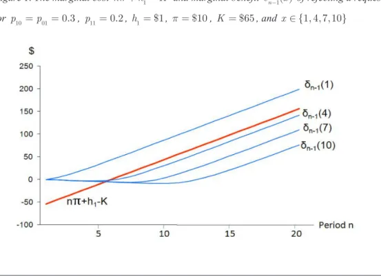
. Motivated by this type of inequalities, the expression dn( ) =x1 V xn( 1-1, )x2 -V x xn( , )1 2 is defined as the marginal benefit of an extra
spare part at facility 1. This benefit does not
depend on x2 for x2 £0 because the backorder cost of x2 units are already incurred until the end of the cycle; this cost is captured by the
np term in (4).
The expression for dn( )x1 differs depend-ing on whether x1³3, x1 = 2, or x1 = 1. By u s i n g ( 3 ) , ( 4 ) , ( 5 ) , a n d dn( ) =x1 V xn( 1-1, )x2 -V x xn( , )1 2 , we obtain x1³3, (10) (11) +p n01[ π+h1−min{K+δn−1( = 1),x1 nπ+h1}]. (12) If xni x x n h K i n i i :=max{ ∈N δ: −1( ) > π+ − }
is the hold-back level for service facility i , we can prove the next theorem; see Appendix B.
Theorem 1i) It is optimal to reject
(respec-tively, accept) the transshipment request when xi £xni (respectively, x x
i n i
level is finite at facility i if and only if
n≥K/ (p+hi).
ii) The hold-back levels are decreasing in the remaining number n of periods:
…
xi xi x
n i
1³ 2³ ³ .
iii) V z zN( , )1 2 is convex for z z1, 2Î N . An interesting question is whether facility 1 holds back more or less inventory towards the end of a replenishment cycle. On one hand, facility 1 may hold back more inventory early in the cycle to meet more of the system demand later in the cycle. On the other hand, backorder costs and hence the savings that can be achieved with transshipment are higher early in the cycle. Thus, there are intuitive reasons for low and high hold-back levels early in the cycle and it deserves an analytical investigation. This ques-tion is answered formally by Theorem 1ii. According to Theorem 1ii, if there are stock-outs in two consecutive periods at facility 2, it
costs less for the system to transship for the first stock-out than the second. This is because the marginal benefit of rejecting a request (value of an extra unit of inventory) increases slower from n to n + 1 remaining periods than the cost of rejecting a request
np +h1−K ; see Figure 1. Since the cost VN
in (9) of the replenishment problem is convex from Theorem 1iii, the optimal order-up-to levels can be found easily from the first-order optimality conditions.
3 CoMPuTaTIonal STudy
To quantify the optimal transshipment benefits, we compare the heuristics of no sharing and complete sharing against our transshipment policy (partial sharing). With a no sharing policy, facilities do not share any parts. In a system us-ing complete sharus-ing, a transshipment request is granted every time it is needed and a unit is available at the other facility.Figure 1. The marginal cost np +h1−K and marginal benefit dn-1( )x of rejecting a request for p10 =p01= 0.3, p11= 0.2, h1= $1, p = $10 , K = $65 , and x Î {1, 4,7,10}
Table 1. As demand parameters change, performance of the optimal sharing policy over heuris-tic policies. `` - ” indicates that replenishment levels are the same as Z1* and Z
2 *. P0 Base case h1=h2 = 1, p = 10, K = 75 Optimal
Sharing SharingNo Complete Sharing
p10 p01 p11 r Z Z1* 2 * , SNS(%) ZNS ZNS 1 , 2 S CS(%) ZCS ZCS 1 , 2 0.150 0.150 0.050 0.06 12,12 3.96 - 1.79 -Increasing r P1 0.500 0.500 0.000 -1.0 27,28 3.69 28,28 2.49 -P2 0.375 0.375 0.125 -0.5 28,28 2.11 - 2.67 27,28 P3 0.250 0.250 0.250 0.0 28,28 1.04 - 2.30 -P4 0.125 0.125 0.375 0.5 28,28 0.26 - 1.74 -P5 0.000 0.000 0.500 1.0 28,28 0.00 - 0.00 -Increasing p10 P6 0.05 0.25 6,12 4.27 7,12 1.24 -P7 0.25 -0.05 17,12 3.90 - 2.06 -P8 0.35 -0.15 23,11 3.43 23,12 2.10 -P9 0.45 -0.25 28,11 3.17 28,12 2.14 -Increasing p11 P10 0.15 0.29 17,17 1.74 - 1.77 -P11 0.25 0.38 23,23 0.70 - 1.79 -P12 0.35 0.40 28,28 0.39 - 1.88 -P13 0.45 0.38 33,33 0.22 - 1.92 -Increasing p10-p01 P14 0.05 0.45 0.00 6,28 3.32 7,28 1.61 -P15 0.15 0.35 -0.15 11,23 3.43 12,23 2.10 -P16 0.25 0.25 -0.19 17,17 3.90 - 2.30 -P17 0.35 0.15 -0.15 23,11 3.43 23,12 2.10 -P18 0.45 0.05 0.00 28,6 3.32 28,7 1.61
-For the numerical experiments, parameters are chosen from the automobile service parts industry. The relationships among parameters are determined from our communication with dealers, related studies in the literature, and Internet sources. Most of the after-sales service is provided by dealers; almost 95% of customers served by General Motors Service Parts Opera-tions organization are served through dealers (Wu & Tew, 2005). Based on our personal
com-munication with several automobile dealers, the replenishment cycle is chosen to be a month.
To determine the number of periods N in a cycle and the demand probabilities, we con-sider average monthly car sales. Car parts such as battery, tires, engine block, alternator, engine belt, CV joints, and struts are normally replaced only a few times within the 10 years after the sale of a car. Indeed, some of these parts last more than the car itself. We suppose that a
Table 2. As cost parameters change, performance of the optimal sharing policy over heuristic policies. `` - ” indicates that replenishment levels are the same as Z1* and Z
2 *. P0 Base case p10=p01= 0.15, p11= 0.05 Optimal
Sharing SharingNo Complete Sharing
h1 h2 K p Z Z1* 2 * , SNS(%) ZNS ZNS 1 , 2 S CS(%) ZCS ZCS 1 , 2 1 1 75 10 12,12 3.96 - 1.79 -Increasing h1, h2 P19 0.1 0.1 16,16 2.33 - 5.15 -P20 0.4 0.4 13,14 3.06 14,14 3.23 14,14 P21 1.2 1.2 11,12 4.29 12,12 1.53 11,11 P22 1.5 1.5 11,11 4.26 - 1.20 -Increasing p P23 6 11,11 1.95 - 3.37 -P24 8 11,11 3.48 12,12 2.33 -P25 12 12,12 5.31 - 1.37 -P26 14 12,13 5.42 13,13 1.07 -Increasing K P27 45 11,12 6.13 12,12 0.42 -P28 55 12,12 5.27 - 0.81 -P29 90 12,12 3.11 - 2.64 -P30 100 12,12 2.62 - 3.26
-single car creates a -single demand for a spe-cific car part in our base case. We find month-ly U.S. car sales publicized on manufacturer web sites and by automotive data collectors. For example, GMinsidenews.com (2007) and Toyota.com (2007a) report that Elantra and Corolla, respectively, had U.S. sales of 9,665 and 25,815 cars in March 2007. To obtain aver-age monthly sales per dealer, we divide the
sales figures by the number of dealers, which is 695 for Hyundai (Hyundai-Motor.com, 2007) and 1481 for Toyota (Toyota.com, 2007b) in the U.S. We find that an average Hyundai or Toyota dealer, respectively, sells 14 Elantras or 17 Corollas per month. The average monthly sales of 14 and 17 are covered by our param-eter values in the numerical experiments. When
N = 60, each period is half of a working day
Figure 2. with N = 30 for p10=p01= 0.3, p11= 0.15, h1 = $0.9, p = $9 , K = $60
for a dealer that is open for 30 days a month. I n o u r b a s e c a s e i n Ta b l e 2 ,
p11+p10=p11+p01= 0.2, which indicates an expected monthly part demand of 12 at each dealer. For the rest of the numerical experiments,
p11+p10 and p11+p01 vary between 0.1 and 0.6, which leads to a monthly demand between 6 and 36.
When the monetary unit is scaled to have a holding cost of unity, we can specify p / h and K h/ ratios. To find reasonable p / h values, we checked some literature. For ex-ample, Cachon (2001) uses 5 and 20; Simchi-Levi and Zhao (2003) use values between 4.75 and 19.75; Zhao et al. (2005) use 100; Tagaras and Vlachos (2002) use 50 and 100. In our base case, p / h is 10. To study problem instances with various parameter values, the ratio ranges over (6,100). To choose a reasonable K h/ ratio, we again follow the literature. We con-sider the ratio Nh K/ of the holding cost per cycle to the transshipment cost. In Tagaras and Vlachos (2002), this ratio is taken as 1.5 and 0.75. In our base case, this ratio is
Nh K/ = 60 * 1 / 75 = 0.8 and ranges over (0.1,1.3) within the experiments, which is consistent with Tagaras and Vlachos (2002).
N should be chosen to be large enough to guarantee at most one demand at each facility in each period. With monthly demands about 15, N = 30 is a reasonable choice. To be on the safe side, we use N = 60 . The choice of
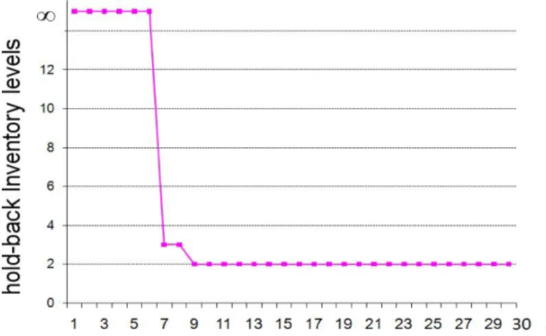
N may seem somewhat arbitrary but it does not affect the hold-back levels much, so it does not lead to an inconsistency between these levels. For example, Figure 2 and Figure 3 il-lustrate the hold-back levels at facility 1 for a single problem instance with two significantly different choices of N , 30 and 90. When N is increased by a factor of three, per period costs and demand probabilities are decreased by a factor of three; p10, p01, p11, h1, and p in Figure 3 are one third of the values in Figure
2. In view of these figures, hold-back levels do not change much with N . For example, xn1 = 3
for about 7£ £n 8 when N = 30 . Also xn1 = 3 for 20£ £n 27 when N = 90 .
Given that 7£ £n 8 for N = 30 corresponds to 21£ £n 24 for N = 90 , we demonstrate that increasing N significantly may change the hold-back pattern only slightly. In real-life implementations, the IM chooses N after analyzing the historical demand data. So the IM can always ensure with a large N that there is at most one demand per period.
The cost V Z ZN( , )1 2 with optimal ( , )1* 2 * Z Z
is denoted by V*. The cost under no sharing
and complete sharing is obtained by, respec-tively, setting xn1 =xn2 = ¥ and x x
n n
1 = 2= 0
for each period n . Let these costs be VCS and
VNS. Clearly V VCS, NS ³V*. We report the
percent cost savings SCS and SNS obtained by
o p t i m a l t r a n s s h i p m e n t s : SNS V V V CS CS = ( - *) / * 100 a n d SNS = (VNS -V*) /VNS * 100. Z 1 and Z2
values are also calculated optimally under the heuristic policies. Thus the ZiNS and Z
i CS
val-ues denote the optimal replenishment valval-ues under each heuristic setting, no sharing and complete sharing, respectively.
Table 1 and Table 2 have a total of 31 problem instances, named from P0 to P30, which are used to illustrate the performance of optimal sharing via comparisons with heuristics of complete and no sharing. In each instance, the purpose is to alter some parameter values from those in the base case to see the effect of the altered parameter(s) on the benefits of op-timal sharing over heuristic policies. In Table 1 and Table 2, a parameter column is blank if the value of the parameter is equal to its base case value. The base case is problem P0 where N = 60 , h1=h2 = $1, p = $10 ,
K = $75, p10= 0.15, p01= 0.15, and p11= 0.05. Since p00= 1 -p10-p01-p11, we have p00= 0.65 in the base case.
In problems P1-P5 of Table 1, the key quantity of interest is the effect of demand cor-relation r on the savings SCS and SNS. To
alter the demand probabilities parametrically as r changes, set p p p p 00 01 10 11 =1 4 1 0 0 1 1 4 0 1 1 0 + + − r r . It is an algebraic exercise to check that these probabilities when plugged into the cor-relation formula (1) yield the corcor-relation r . To study the effect of correlation on performance,
r is set to different values from the set { 1, 0.5, 0, 0.5,1}- - and the corresponding demand parameters are obtained from the above equation. This equation also ensures that
p10+p11= 0.5 and p01+p11= 0.5 through-out P1-P5. Thus, the results can only be at-tributed to the change in demand correlation.
The results indicate that a negative cor-relation between service part demands yields higher gains from optimal transshipments. This inference can be made in view of higher SNS
and SCS for r < 0 . Most of the parameter
changes in Table 1, except for those in r , cause
SNS and SCS to move in opposite directions.
When demands are perfectly correlated, the costs of complete sharing and no sharing heu-ristics coincide with the optimal cost. In this case, both facilities have leftover inventory or both stock out, either of which renders trans-shipments useless. This observation is sup-ported by Herer et al. (2006), Dong and Rudi (2004), and Zhang (2005) under various trans-shipment and replenishment settings. On the other hand, even when demands are
moder-ately correlated, P0, P2, P3, and P4 indicate considerable gains provided by the optimal transshipment policy.
In P6-P18, demand rates are altered in several different ways to model the various scenarios. The probability p10 of demand at facility 1 is increased in P6-P9 to study facil-ity 1 that serves a larger market size. When facility 1 is larger, the IM orders more for facil-ity 1. The benefit of optimal transshipments remain sizable in P6-P9. It appears that no sharing performs relatively better when facil-ity 1 grows. When facilfacil-ity 1 is substantially larger than facility 2, facility 1 cannot rely on limited inventory at facility 2 to handle stock outs. This is why the benefit of sharing drops. This drop becomes slightly stronger when the demand correlation is higher as illustrated in P10-P13. Lastly, facility 1 is made larger while facility 2 is made smaller in P14-P18 to see the effect of market size asymmetry on the perfor-mance. Optimal transshipments reduce the cost most when the facilities have symmetric market sizes. If the IM has several facilities to pair for transshipment purposes, he should pair facilities with the same/similar market sizes to obtain most benefits.
In Table 2, the effects of cost parameters on the benefits of the optimal transshipments are depicted. From P19-P26, increases in hold-ing and backorder costs amplify the benefit of optimal transshipments. This observation rein-forces the fact that our transshipments reduce both leftover inventory and stock outs. That is why the optimal transshipments perform rela-tively better when the leftover inventory (hold-ing) cost or stock out (backorder) cost is high. On the other hand, when the cost of transship-ping K increases in P27-30, it is optimal to use transshipments more selectively. This brings the cost of optimal transshipments closer to the cost of no sharing and increases the cost savings w.r.t. the cost of complete sharing.
Results in Table 1 and Table 2 illustrate that sizable cost savings can be achieved by using optimal transshipment policies instead of a no sharing or complete sharing heuristic.
The average cost savings are 3% and 2%, re-spectively, over no sharing and complete shar-ing and the maximum cost savshar-ing exceeds 6% and 5%, respectively. We depict these savings and the inferences made from Table 1 and Table 2 in Figure 4. These heuristics are drawn as balloons at the heights of SNS and SCS from
the ground that represents the optimal trans-shipments. The balloons are pulled towards the ground by weights that represent problem pa-rameters. For example, when h h1, 2, or p is large, the cost of complete sharing approaches the cost of optimal sharing with transshipments.
Finally, numerical experiments in Table 1 and Table 2 indicate that transshipment policy, be it optimal or heuristic, has little effect on the replenishment quantities. One may expect that the coordination among facilities through transshipments would decrease the inventory levels in the system. Increasing inventory levels with transshipments is unexpected, but it is an observation often made by previous transship-ment studies such as Grahovac and Chakravarty
(2001), Zhao et al. (2005), and Zhang (2005). All of our instances have a smaller replenish-ment quantity in the case of optimal sharing than those in the case of no sharing. However, replenishment quantities with optimal sharing are smaller than those with complete sharing in P20, and they become larger in P21. Thus, transshipments among facilities does not neces-sarily reduce the inventory in the system.
4 a SInGlE ParaMETEr
hEurISTIC For
TranSShIPMEnTS
Our hold-back computations are based on dif-ference equations. They are simple and fast to run. They can be implemented in a simple Excel spreadsheet to obtain the optimal hold-back levels. In practice, the hold-hold-back levels should be computed by the IM and passed to the service facilities. Most managers are familiar enough with spreadsheets to be able to compute the hold-back levels. Once hold-back levels
Figure 4. Savings SNS is reduced by parameters K p p, ,
10 11, savings S
CS is reduced by h h
1, ,2 p. Both savings are reduced by demand correlation and market size asymmetry.
are available, all that a facility should do is to compare the current inventory level against the hold-back level during transshipment con-sideration. As long as the problem parameters remain the same over the replenishment cycles, the hold-back levels computed once can be used multiple times.
Despite the ease of computation and imple-mentation of the hold-back level-based trans-shipments, some implementers may insist on basing the transshipment decisions on a single parameter for facility i rather than N param-eters of hold-back levels { : 1xni £ £n N}. The range for hold-back levels is wide, ranging from zero to infinity, so collapsing, say by averaging, such a wide range to a single num-ber is a crude approximation. Instead of a single number, we represent the optimal trans-shipment policy equivalently in terms of hold-back times that range from 1 to N .
Define the hold-back time
nxi n x x
n i
:=max{ : £ }
that denotes the number of remaining periods in a cycle during which it is not optimal to grant a transshipment at retailer i with inventory level x . If both x and n had been continuous, nxi could have been interpreted
as the inverse function of xni. Then we would
have x x
nxi i
=
. In our discrete case, we have
x x x nxi i nxi i +1< ≤ . Since xn i is decreasing in n
by Theorem 1ii, so is nxi in x . For any x and
n, we can show that [n£nxi] if and only if [x£xni]. Therefore, rejection of a transship-ment request can be equivalently based on [n£nxi], as Archibald et al. (1997) do in a different setting than ours. Unlike Archibald et
al., we have decreasing nx
i in x (or
equiva-lently decreasing xn
i in n ), which implies that
the inventory level of facility i crosses xn i only
once in a replenishment cycle. Let the period when that crossing happens be Ni, which is a
random variable as it depends on demands that drive the drop in the inventory level. The re-quests are rejected for n N£ i and they are
accepted for n N> i.
Since Ni is a demand dependent random
variable, it cannot be set equal to a single num-ber at the beginning of a replenishment cycle before demands materialize. Thus, a policy based on N is not implementable. To gain implementability, we give up optimality. A heuristic is built with a parameter ni, where
requests are rejected for n n£i. The
subopti-mality of the heuristic is because accept/reject decisions are specified by ni, independent of
the actual demand materialization during a cycle. However, demand parameters are used to calculate ni, so the heuristic, despite
ignor-ing demand materialization, captures demand expectations and correlations.
The computation of ni is not
straightforward although we know that
ni K h
i
≥ / (p+ ) from Theorem 1i. For
N = 60, enumeration is used by considering
ni K h i = / (p+ ) +2, ni K h i = / (p+ ) +10, and ni K h i = / (p+ ) +16 for i Î {1,2} . To test the performance of this heuristic against our optimal transshipment policy, 1000 problem instances were generated with uni-formly chosen parameter values from the fol-lowing
hi Î (0.7,1.5), p Î (5,12), and K Î (60,100). Each instance is solved to find the optimal ordering levels by using the optimal hold-back policy and by using the heuristic with ni. Thus
the order quantities are optimized even in the heuristic pooling policy. If n is appended as a decision variable to the cycle cost,
(13) The increase in the cycle cost by using the heuristic policy instead of the optimal policy is calculated for each problem instance. Then average cost increases are calculated over 1000 problem instances for each value of n . The heuristic policy results in an average cost increase of 0.71%, 1.10%, and 1.81% when the heuristic is run with, respectively, n1=n2 =K/ (p+hi) +2,
n1=n2 =K/ (p+hi) +10, and
n1=n2 =K/ (p+hi) +16. Even the best
value of n1 =n2 results in non-negligible
extra cost.
The heuristic can be improved by
simul-taneously optimizing over n , z1, and z2. More specifically, for a given problem instance, the cost in (13) is minimized over three variables, n, z1, and z2. Although this heuristic slightly improves the costs, it is based on enumeration that must be done in the absence of analytical structural results. Our optimal transshipment policy has a nice separation property that allows us to compute the optimal hold-back levels without knowing optimal values of Z1 and Z2. There is no such separation structure to exploit in the heuristic computations. From computation complexity alone, we suggest using the optimal hold-back levels (times) rather than the complicated heuristic.
The lack of separation in the heuristic is troublesome not only for computation but also for implementation. Optimal ni is not robust
against variations in Z1 or Z2. In practice, because of quality problems, spoilage, theft, or damage in transport, the units received in good condition at the beginning of a cycle can be less than the optimal order quantities. In this case, a different optimal ni value must be
computed in every cycle with the actual values of inventory available at the service facilities. This further complicates the computations/ implementation of the heuristic.
5 ConCludInG rEMarkS
In this paper, we propose a nested model to make optimal replenishment and transshipment deci-sions. The transshipment model is appropriate for service part supply chains as it considers demand dynamics, sparsity, and dependence, as well as multiple transshipments per cycle. The demand model is fairly general; its special as well as limiting cases are studied in trans-shipment and other settings in the literature. For this demand model, we obtain an optimal transshipment (inventory sharing) policy, which is based on hold-back levels.The optimal sharing policy is compared to the heuristic policies of no sharing and com-plete sharing. The cost differences among these policies depend on parameter values and are pictured in Figure 4. A practitioner, who must implement either no sharing or complete shar-ing, can choose either one of these heuristics by examining cost differences under the parameter values that resemble his/her real-life setting. We also investigate heuristics based on a single parameter, a critical hold-back time. Computa-tion of this critical time is not simple. Moreover, heuristics result in higher system costs that can be reduced by using the optimal policy. Conse-quently, we advocate the implementation of the hold-back level-based optimal transshipment policy. Computation of hold-back levels, say
in a spreadsheet, is easy. Once these levels are communicated to the service part facilities, the implementation is easy as well, which does not require an IM’s real time oversight. The hold-back levels are robust against changes in the replenishment quantities.
aCknowlEdGMEnT
We thank P. Schunck, BMW of Dallas, for help-ing us to better understand transshipments in the automobile industry. The formulation stage of this research is supported by 2008 summer research grants given to the second and third authors by the School of Management, the University of Texas at Dallas.
rEFErEnCES
Anupindi, R., Bassok, Y., & Zemel, E. (2001). A General Framework for the Study of Decentralized Distribution Systems. Manufacturing & Service Op-erations Management, 3(4), 349–368. doi:10.1287/ msom.3.4.349.9973
Archibald, T. W., Sassen, S. A. E., & Thomas, L. C. (1997). An Optimal Policy for a Two Depot Inventory Problem with Stock Transfer. Management Science, 43(2), 173–183. doi:10.1287/mnsc.43.2.173 Axsäter, S. (1990). Modelling Emergency Lateral Transshipments in Inventory Systems. Manage-ment Science, 36(11), 1329–1338. doi:10.1287/ mnsc.36.11.1329
Boone, C. A., Craighead, C. W., & Hanna, J. B. (2008). Critical Challenges of Inventory Management in Service Parts Supply: A Delphi Study. Operations Management Research, 1, 31–39. doi:10.1007/ s12063-008-0002-2
Cachon, G. P. (2001). Stock Wars: Inventory Com-petition in a Two-Echelon Supply Chain with Mul-tiple Retailers. Operations Research, 49, 658–674. doi:10.1287/opre.49.5.658.10611
Çakanyıldırım, M., Royal, A. J., & Beckett, J. (2008). Forecasting Sales for Heating, Ventilating, and Air Conditioning (HVAC) Products (Working Paper). Dallas, TX: The University of Texas at Dallas, School of Management.
Çömez, N., Stecke, K. E., & Çakanyıldırım, M. (2009a). Multiple In-Cycle Transshipments with Positive Delivery Times (Working Paper). Dallas, TX: The University of Texas at Dallas, Richardson. Çömez, N., Stecke, K. E., & Çakanyıldırım, M. (2009b). Optimal Transshipments and Orders: A Tale of Two Competing and Cooperating Retailers (Working Paper). Dallas, TX: The University of Texas at Dallas, Richardson.
Complaints.com. (2009a). Retrieved April, 25, 2009, from www.complaints.com/2007/may/12/ Sears_Kenmore_dishwasher__144654.htm Complaints.com. (2009b). Retrieved April, 25, 2009, from www.complaints.com/2007/november/30/ MATTRESS_WAREHOUSE______ 155511.htm Complaints.com. (2009c). Retrieved April, 25, 2009 from www.complaints.com/2007/september/6/ Best_Buy_complaint_152271.htm
Dong, L., & Rudi, N. (2004). Who Benefits from Transshipment? Exogenous vs. Endogenous Whole-sale Prices. Management Science, 50(5), 645–657. doi:10.1287/mnsc.1040.0203
Flint, P. (1995). Too Much of a Good Thing: Better Inventory Management Could Save the Industry Millions While Improving Reliability. Air Transport World, 32(9), 103–106.
Gminsidenews.com. (2007). March U.S. Car Sales By Model. Retrieved April 25, 2009, from http:// www.gminsidenews.com/forums/showthread. php?t=29676
Grahovac, J., & Chakravarty, A. (2001). Sharing and Lateral Transshipment of Inventory in a Sup-ply Chain with Expensive Low-Demand Items. Management Science, 47(4), 579–594. doi:10.1287/ mnsc.47.4.579.9826
Herer, Y. T., & Rashit, A. (1999). Lateral Stock Trans-shipments in a Two-Location Inventory System with Fixed and Joint Replenishment Costs. Naval Research Logistics, 46, 525–547. doi:10.1002/(SICI)1520-6750(199908)46:5<525::AID-NAV5>3.0.CO;2-E Herer, Y. T., Tzur, M., & Yucesan, E. (2006). The Multi-Location Transshipment Problem. IIE Transactions, 38(3), 185–200. doi:10.1080/07408170500434539 Hyundai-Motor.com. (2007). News & Events. Retrieved April 25, 2009, from http://www.world-wide.hyundaimotor.com/common/html/about/ news_event/press_read_2006_01.html
Kennedy, W. J., Patterson, J. W., & Fredendall, L. D. (2002). An Overview of Recent Literature on Spare Parts Inventories. International Journal of Production Economics, 76, 201–215. doi:10.1016/ S0925-5273(01)00174-8
Krishnan, K. S., & Rao, V. R. K. (1965). Inventory Control in N Warehouses. Journal of Industrial Engineering, 16, 212–215.
Kukreja, A., Schmidt, C. P., & Miller, D. M. (2001). Stocking Decisions for Low-Usage Items in a Multilocation Inventory System. Manage-ment Science, 47(10), 1371–1383. doi:10.1287/ mnsc.47.10.1371.10263
Lee, H. L., & Tang, C. S. (1998). Variability Reduc-tion Through OperaReduc-tions Reversal. Management Science, 44(2), 162–172. doi:10.1287/mnsc.44.2.162 Lee, T. C., & Hersh, M. (1993). A Model for Dynamic Airline Seat Inventory Control with Multiple Seat Bookings. Transportation Science, 27(3), 252–265. doi:10.1287/trsc.27.3.252
Narus, J. A., & Anderson, J. C. (1996, July-August). Rethinking Distribution: Adaptive Channels. Har-vard Business Review, 112–120.
Ranaweera, C., & Neely, A. (2003). Some Mod-erating Effects on the Service Quality-Customer Retention Link. International Journal of Opera-tions & Production Management, 23(2), 230–248. doi:10.1108/01443570310458474
Regattieri, A., Gamberi, M., Gamberini, R., & Manzini, R. (2005). Managing Lumpy Demand for Aircraft Spare Parts. Journal of Air Transport Management, 11(6), 426–431. doi:10.1016/j.jairtra-man.2005.06.003
Righter, R., & Shanthikumar, J. G. (2001). Opti-mal Ordering of Operations in a Manufacturing Chain. Operations Research Letters, 29, 115–121. doi:10.1016/S0167-6377(01)00091-8
Rudi, N., Kapur, S., & Pyke, D. F. (2001). A Two-cation Inventory Model with Transshipment and Lo-cal Decision Making. Management Science, 47(12), 1668–1680. doi:10.1287/mnsc.47.12.1668.10235 Shahla Rostamidehbaneh, F. F. (2006). After Sales Service Necessity and Effectiveness. Unpublished master’s thesis, Lulea University of Technology, Sweden.
Simchi-Levi, D., & Zhao, Y. (2003). The Value of In-formation Sharing in a Two-Stage Supply Chain with Production Capacity Constraints. Naval Research Logistics, 50, 888–916. doi:10.1002/nav.10094 Sošić, G. (2006). Transshipment of Inventories Among Retailers: Myopic vs. Farsighted Stabil-ity. Management Science, 52(10), 1493–1508. doi:10.1287/mnsc.1060.0558
Tagaras, G. (1999). Pooling in Multilocation Periodic Inventory Distribution Systems. Omega . Interna-tional Journal of Management Science, 27, 39–59. Tagaras, G., & Cohen, M. A. (1992). Pooling in Two-Location Inventory Systems with Non-Negligible Replenishment Lead Times. Management Science, 38(8), 1067–1083. doi:10.1287/mnsc.38.8.1067 Tagaras, G., & Vlachos, D. (2002). Effectiveness of Stock Transshipment Under Various Demand Distributions and Nonnegligible Transshipment Times. Production and Operations Management, 11(2), 183–198.
Toyota.com. (2007a). Toyota Reports October Sales. Retrieved April 25, 2009, from http://www.toyota. com/about/news/ corporate/2007/11/01-1-sales.html Toyota.com. (2007b). Toyota in the United States. Retrieved April 25, 2009, from http://www.toyota. com/about/our_business/at_a_glance/our_numbers/ index.html
Wu, P., & Tew, J. D. (2005). Collaborations in the Automotive After-sales Supply Chain. In Proceed-ings of the Sixteenth Annual Conference of POMS, Chicago, IL.
Xu, K., Evers, P. T., & Fu, M. C. (2003). Estimating Customer Service in a Two-Location Continuous Review Inventory Model with Emergency Transship-ments. European Journal of Operational Research, 145, 569–584. doi:10.1016/S0377-2217(02)00158-3 Zandi, M. (2008, December 4). The State of the Domestic Auto Industry: Part II. Washington, DC: Testimony Before the U.S. Senate Committee on Banking, Housing, and Urban Affairs.
Zhang, J. (2005). Transshipment and Its Impact on Supply Chain Members’ Performance. Manage-ment Science, 51(10), 1534–1539. doi:10.1287/ mnsc.1050.0397
Zhang, X. (2007). Inventory Control Under Temporal Demand Heteroscedasticity. European Journal of Operational Research, 182, 127–144. doi:10.1016/j. ejor.2006.06.057
Zhao, H., Deshpande, V., & Ryan, J. K. (2005). Inven-tory Sharing and Rationing in Decentralized Dealer Networks. Management Science, 51(4), 531–547. doi:10.1287/mnsc.1040.0321
Zhao, H., Ryan, J. K., & Deshpande, V. (2006). Emergency Transshipments in Decentralized Dealer Networks: When to Send and Accept Transshipment Requests. Naval Research Logistics, 53, 547–567. doi:10.1002/nav.20160
Zhao, H., Ryan, J. K., & Deshpande, V. (2008). Optimal Dynamic Production and Inventory Trans-shipment Policies for a Two-Location Make-to-Stock System. Operations Research, 56(2), 400–410. doi:10.1287/opre.1070.0494
EndnoTE
1 We use increasing and decreasing loosely to, respectively, mean decreasing and non-increasing.
Nagihan Çömez is an assistant professor of Operations Management at the Faculty of Business Administration at Bilkent University. She holds a B.S. degree in Industrial Engineering from Bogazici University, Turkey and an M.S. degree in Supply Chain Management and a Ph.D. degree in Operations Management from the University of Texas at Dallas. She is an INFORMS member. Her research interests focus on inventory management and coordination in retailer sys-tems, particularly on inventory sharing, inventory-pricing models, and supply chain scheduling. Kathryn E. Stecke is the Ashbel Smith Professor of Operations Management at the University of Texas at Dallas. She received an M.S. in Applied Mathematics and an M.S. and Ph.D. in Industrial Engineering from Purdue University. She was the founding Editor-in-Chief of the International Journal of Flexible Manufacturing Systems and is Editor-in-Chief of Operations Management Education Review. She has served on both the INFORMS and POMS Board of Directors. She is an INFORMS Fellow. She has authored papers in various journals including The FMS Magazine, Material Flow, International Journal of Production Research, Journal of Marketing Channels, Operations Management Education Review, European Journal of Operational Research, IIE Transactions, Annals of Operations Research, Management Science, Production and Opera-tions Management, Manufacturing and Services OperaOpera-tions Management, OperaOpera-tions Research, International Journal of Manufacturing Research, and others.
Metin Çakanyıldırım is an associate professor at the School of Management at the University of Texas at Dallas. He received his B.S. in Industrial Engineering from Bilkent University, Turkey, his M.S. in Management Science from University of Waterloo, Canada, and his Ph.D. in Operations Research from Cornell University. He is a member of INFORMS, POMS, and IIE. His research interests include inventory and capacity management, risk management, and information security.
aPPEndIx a: ParaMETEr ESTIMaTIon
The first parameter to estimate is the number of periods N in a replenishment cycle. If N is too small, there will be more than one demand occurrence in some periods at some facilities. To avoid this, first consider the demand at facility 1 and increase N or equivalently shorten a pe-riod until there is at most one demand in each pepe-riod at facility 1. This gives an estimate of N based on facility 1 demand. We can obtain a similar estimate from facility 2 and set ˆN equal to the maximum of these two estimates.
ˆ ˆ ˆ ˆ m1= (N p01+p11) and m2 = (N p10+p11). (14) ˆ r = ( )( )( )( ), 00 11 01 10 10 11 01 00 01 11 10 00 p p p p p p p p p p p p − + + + + ˆ ˆˆ ˆˆ ˆˆ ˆˆ ρ µ1 µ2 µ1 µ2 00 11 01 10 1 1 = = N N -N -N p p -p p p11 p p01 11 p p10 11 p112 p p 01 10. - - - -ˆ ˆ ˆ ˆ m m1 2 01 11 10 11 11 2 01 10 = . N N p p +p p +p +p p p N N N N N N 11 1 2 1 2 1 2 =ρˆ µˆˆ µˆˆ 1−µˆˆ 1−µˆˆ +µ µˆˆ ˆˆ. p N N N N N N N 01= 1 1 2 1 1 1 2 1 2 ˆ ˆ ˆ ˆ ˆ ˆ ˆ ˆ ˆ ˆ ˆ ˆ ˆ ˆ ˆ µ ρ µ µ µ µ µ µ - - - -p N N N N N N N 10 2 1 2 1 2 1 2 =µˆˆ -ρˆ µˆˆ µˆˆ 1-µˆˆ 1-µˆˆ -µ µˆˆ ˆˆ.
The last three equalities allow us to estimate the demand parameters in terms of the empirical statistics ˆ ˆm m1, 2, and ˆr .
aPPEndIx b: ProoFS
Lemma 1 is a property of the difference of two min functions. It is used for proving Theorem 1ii.
Lemma 1For any four real numbers a b c, , , and d ,
min{a−c b, −d}≤min{ , }a b −min{ , }c d ≤max{a−c b, −d}. Proof. min{a,b}-min{c,d} = min{a,b}+max{-c,-d} = min{a+max{-c,-d},b+max{-c,-d}}≥min{a-c,b-d}, min{ , }a b -min{ , }c d =min{ , }a b +max{ ,− −c d}
=max{− +c min{ , },a b − +d min{ , }}a b ≤max{a−c b, −d}.
Proof of Theorem 1i .To prove the first statement in i), first show that the marginal benefit is
decreasing in inventory level: dn( )x1 ≤dn(x1−1) for x1Î N . Induction is used on the remain-ing number of periods n . Since d0( ) = 0× , we have that d0( )x1 ≤d0(x1−1), for n = 0 .
1|1= {1,if nπ+h1−K<δn−1( ); 0,x otherwise},
1|2= {1,if δn−1( )x ≤nπ+h1−K<δn−1(x−1); 0,otherwise},
1|3= {1,if δn−1(x−1)≤nπ+h1−K<δn−1(x−2); 0,otherwise}, 1|4= {1,if δn−1(x−2)≤nπ+h1−K<δn−1(x−3); 0,otherwise},
1|5= {1,if δn−1(x−3)≤nπ+h1−K; 0,otherwise},
For x1³4, (10) can be rewritten for inventory levels x1 and x1-1 by using the following