A HYBRID INVENTORY CONTROL POLICY FOR
MEDICAL SUPPLIES IN HOSPITALS
A THESIS
SUBMITTED TO THE DEPARTMENT OF INDUSTRIAL
ENGINEERING
AND THE INSTITUTE OF ENGINEERING AND SCIENCE
OF BILKENT UNIVERSITY
IN PARTIAL FULFILLMENT OF THE REQUIREMENTS
FOR THE DEGREE OF
MASTER OF SCIENCE
By
Gökçe Akın
ii
I certify that I have read this thesis and that in my opinion it is full adequate, in scope and in quality, as a dissertation for the degree of Master of Science.
___________________________________ Asst. Prof. Dr. Osman Alp (Advisor)
I certify that I have read this thesis and that in my opinion it is full adequate, in scope and in quality, as a dissertation for the degree of Master of Science.
___________________________________ Asst. Prof. Dr. Murat Fadıloğlu
I certify that I have read this thesis and that in my opinion it is full adequate, in scope and in quality, as a dissertation for the degree of Master of Science.
______________________________________ Asst. Prof. Dr. Banu Yüksel Özkaya
Approved for the Institute of Engineering and Sciences:
____________________________________ Prof. Dr. Levent Onural
iii
ABSTRACT
A HYBRID INVENTORY CONTROL POLICY FOR MEDICAL
SUPPLIES IN HOSPITALS
Gökçe Akın
M.S. in Industrial Engineering Advisor: Asst. Prof. Dr. Osman Alp
July, 2010
In this thesis, we consider the inventory control problem of medical supplies that arises in a particular hospital environment. The items are stored in nursing stations from where they are retrieved by the nurses and used for the needs of in-patients or out-patients. The nursing stations are replenished from a central warehouse. Items are moved between the hospital’s central warehouse and the nursing stations by a capacitated porter cart. In the representative nursing station that we analyze, the need for the medical supplies by the in-patients can arise at any time during day or night. It is possible to replenish the nursing stations during the day time on a continuous scale; however, this is not possible after-hours because the warehouse operates only during regular working hours. For this particular setting, we propose a hybrid inventory control policy which consists of a continuous review joint replenishment policy to manage the day time demand and a periodic review policy to manage the night time demand. The prior performance measure is set to satisfy the target service levels in the nursing stations. For a special case of the problem with a single item, we develop exact expressions to estimate the policy parameters. For the multi-item case, we analyze the impact of the policy parameters on the service level targets by simulating a representative system under different scenarios. Finally, we analyze a sample data collected from a nursing station and prescribe methods to determine the policy parameters.
Keywords: Medical supplies, inventory control, joint replenishment, service level, health care system
iv
ÖZET
HASTANELERDEKİ TIBBİ SARF MALZEMELERİ İÇİN KARMA
ENVANTER KONTROL POLİTİKASI
Gökçe Akın
Endüstri Mühendisliği Yüksek Lisans Tez Yöneticisi: Yrd. Doç. Dr. Osman Alp
Temmuz, 2010
Bu tezde, incelediğimiz bir hastane ortamında kullanılan tıbbi sarf malzemeleri için bir envanter kontrol problemi incelenmiştir. Bu hastanede tıbbi sarf malzemeleri her katta bulunan hasta bakım istasyonlarında belirli miktarlarda tutulmakta ve kat hemşireleri tarafından yatan veya ayakta tedavi gören hastalar için kullanılmaktadır. Hasta bakım istasyonları kapasiteli bir el arabası kullanılarak ana depodan yeniden doldurulmaktadır. Ele alınan örnek katta tıbbi sarf malzemeleri için gün içerisinde veya gece herhangi bir saatte talep görülebilmektedir. Gün içerisinde hasta bakım istasyonları herhangi bir zamanda sürekli olarak yeniden doldurulabilirken; çalışma saatleri dışında ana depo kapalı olduğu için bu mümkün olmamaktadır. Böyle bir sisteme uygun olarak karma bir envanter politikası önerilmiştir. Bu politikada gün içerisindeki envanter kontrolü için sürekli yeniden gözden geçirilen toplu sipariş politikası önerilirken; gece için bir dönemsel gözden geçirme politikası önerilmiştir. Performans kriteri, hedeflenen hizmet düzeyinin sağlanması olarak belirlenmiştir. Özel bir durum olarak tek ürünlü sistemde politika parametrelerin elde edilebilmesi için kesin ifadeler türetilmiştir. Çok ürünlü sistem için ise politika parametrelerinin hizmet düzeyi üzerindeki etkileri gözlemlemek için sistem farklı senaryolar altında simüle edilmiş ve parametre kestirimi için yöntemler önerilmiştir. Son olarak, hastaneden alınan örnek data incelenmiş ve önerilen kestirim yöntemleri uygulanıp değerlendirilmiştir.
Anahtar sözcükler: Tıbbi sarf malzemeler, envanter kontrolü, toplu sipariş, hizmet düzeyi, sağlık sistemi
v
Acknowledgement
First of all, I would like to express my sincere gratitude to my supervisor Asst. Prof. Dr. Osman Alp for his invaluable guidance and support during my graduate study. He has supervised me with everlasting interest and motivation throughout this study. I would like to thank once more for his encouraging advices on the other academical issues, especially for the last two years.
I am also grateful to Asst. Prof. Dr. Murat Fadıloğlu and Asst. Prof. Dr. Banu Yüksel Özkaya for accepting to read and review this thesis and for their invaluable suggestions.
I would like to thank to Ankara Güven Hospital for letting me to analyze the hospital and providing me the representative data for this study.
I would like to express my sincere thanks to Prof. Dr. İhsan Sabuncuoğlu, Assoc. Prof. Dr. Bahar Yetiş Kara and (once more) Asst. Prof. Dr. Osman Alp, since they have always trusted in me and appreciated my work as their teaching assistant for two years.
I am indebted to my fiance Korhan Aras for his incredible support and encouragement for six years. I am also lucky to have Uğur Cakova as one of my best friends who is ready to listen to me, encourages me with his advices and comes up instant solutions all the time. Additionally, I am thankful to Pelin Damcı (and Mehmet Can Kurt), Gülşah Hançerlioğulları, Hatice Çalık, Ece Demirci, Efe Burak Bozkaya (and Füsun Şahin Bozkaya), Esra Koca, Burak Paç, Can Öz, Yiğit Saç, Emre Uzun and all other friends that I failed to mention here, for their invaluable support and friendship during my graduate study.
Most importantly, I would like to express my deepest gratitude to my family for their endless love and support throughout my life.
vi
Contents
1. Introduction ... 1
2. Literature Review... 6
2.1. OR in Health Care Literature ... 6
2.2. Inventory Control of Medical Supplies ... 7
2.3. Joint Replenishment Policies with an Emphasis on Service Levels ... 8
3. System Description and Data Analysis ... 12
3.1. System Description ... 12
3.2. Data Analysis ... 14
4. Model and Policies ... 25
4.1. Definition of the Inventory Problem ... 25
4.2. Solution Approaches ... 27
4.2.1. Our Proposed Control Policy ... 28
vii
5. Policy Parameters Estimation ... 41
5.1. An Estimation Method to Find Policy Parameters ... 41
5.2. The Simulation Results for the Inventory System ... 46
6. Conclusion ... 58
Appendix A. The Detailed Information of the Items ... 65
viii
List of Figures
1.1. Health care sector supply chain... 2
3.1. Medical supplies inventory system in the hospital ... 13
3.2. Histogram with Gamma fit for the interarrival times of item ID51 ... 18
3.3. Histogram with Gamma fit for item ID51 total demand per night ... 19
3.4. Histogram with Gamma fit for the interarrival times of item ID52 ... 19
3.5. Histogram with Gamma fit for item ID52 total demand per night ... 20
3.6. Histogram with Gamma fit for the interarrival times of item ID122 ... 20
3.7. Histogram with Gamma fit for item ID122 total demand per night ... 21
3.8. Histogram with Gamma fit for the interarrival times of item ID95 ... 21
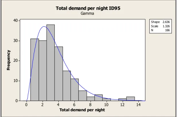
3.9. Histogram with Gamma fit for item ID95 total demand per night ... 22
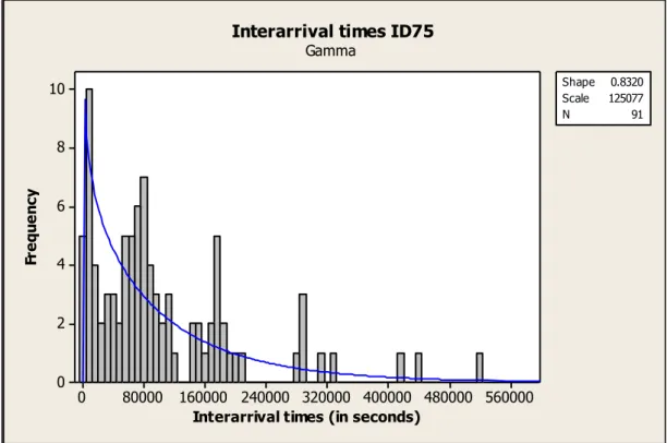
3.10. Histogram with Gamma fit for the interarrival times of item ID75 ... 23
3.11. Histogram with Gamma fit for the interarrival times of item ID112 ... 23
ix
4.2a. First example of the behavior of inventory level over time ... 32
4.2b. Second example of the behavior of inventory level over time... 32
4.3. Illustration of the demand arrivals within for ... 34
B.1. Daily demand distributions for the item ID42 ... 74
B.2. Daily demand distributions for the item ID51 ... 74
B.3. Daily demand distributions for the item ID41 ... 75
B.4. Daily demand distributions for the item ID146 ... 75
B.5. Daily demand distributions for the item ID52 ... 76
x
List of Tables
3.1. Correlation analysis for A items ... 16
3.2. Correlation analysis for B items ... 17
3.3. Distributions of compound parts for A items day-time demands ... 18
3.4. Distributions of compound parts for B items day-time demands ... 22
3.5. Distributions of night-time demands for B items ... 24
4.1. Notation ... 31
5.1. Results for the Scenario 1 ... 53
5.2. Results for the Scenario 2 ... 53
5.3. Results for the Scenarios 3-5... 54
5.4. Results for the Scenario 6 ... 54
5.5. Results for the Scenario 7 ... 55
5.6. Results for the Scenario 8 ... 55
xi
5.8. Results for the Scenarios 10 and 11 where and ... 56
A.1. Six months data for 195 medical items ... 66
1
Chapter 1
Introduction
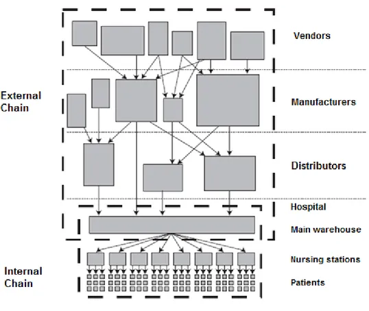
Health care sector supply chains are known to be structurally complicated and are characterized by two chains: an external and an internal chain as shown in Figure 1.1 (Rivard-Royer, et al., 2002). Within this thesis, we do not consider the external chain, instead we mainly focus on the internal chain which consists of the main warehouse, the nursing stations and patients. In the internal chain, the nurses retrieve the necessary items from the nursing stations for the patient needs and the nursing stations are replenished by the main warehouse. Within hospitals, it is the top priority to meet the patient needs on time, and hence inventory management plays a significant role in hospital supply chains. As it is also underlined by Burns et al. (2002), in the hospital supply chains the end users are not customers who are directly paying for the item, but are the patients who create a demand at the nursing stations due to clinical preference. For this reason, cost-benefit analysis or the budget constraints are not considered as the main issue in the inventory management of medical items.
CHAPTER 1. INTRODUCTION
2
Figure 1.1: Health care sector supply chain (Adapted from Rivard-Royer, et al., 2002)
In hospitals, since a patient’s health is the main concern, it is essential to satisfy the patient needs on time. For this reason, throughout this thesis we mainly focus on satisfying required service levels rather than minimizing the cost. Type 2 service level (i.e. fill-rate), which is the proportion of unsatisfied demand, is taken as a performance indicator. In a typical hospital, there are three types of items that can be demanded at anytime: medical supplies, pharmaceuticals and textile items. Injector, syringe, etc. can be given as the examples of medical supplies. Pharmaceuticals include medicines and hygienic liquids, whereas textile items are composed of towels, bed sheets, etc. Certain amounts of medical supplies should be kept close to the point of delivery (nursing stations in our case), from where the nurses retrieve the items for the patient needs. In these places, a variety of these medical supplies need to be hold so that demand, which can occur at anytime during a day, can be met on time.
CHAPTER 1. INTRODUCTION
3
Within our study, we consider the inventory system in a local hospital in Ankara, namely Ankara Guven Hospital. In this hospital, a material tracking system is being used for the medical supplies, since the medical supplies are the most demanded group of items. With the existing material tracking system in the hospital, each medical supply’s actual inventory level throughout the day can be tracked easily. However, neither the responsible personnel in the hospital know, nor this system includes the information of exactly when and how the replenishments should be done at the nursing stations, in order to satisfy the target service levels while not holding excess amount of inventory due to limited storage places. For this reason, we motivate our study on this inventory control problem of Guven Hospital.
Ankara Guven Hospital, founded 36 years ago, is one of the leading institutions of the Turkish health care sector (Ankara Guven Hospital, 2010). The hospital has the certification of ISO 9001:2000 and the certification of Joint Commission International (JCI) accreditation standards. In order to meet the expectations of patients and their companions, the hospital employs over 850 personnel. The hospital was established on 20,000 area. It consists of eight operating rooms and 156 beds. There are five nursing stations, from which in-patients and out-patients are served, and one central warehouse, from which the nursing stations are replenished. Within this thesis, we select the nursing station at Block A 3rd Floor as the representative station, in which 195 different medical supplies are used. For these medical supplies, at the representative nursing station the total daily demand is 240 on the average.
Based on the inventory control problem that arises in Guven Hospital, we consider a multi-item system in which a capacitated porter cart is used for moving items from the main warehouse to the nursing stations. Controlling multiple items in a system, where high service levels are required, is a challenge itself. Additionally, another challenge of our problem is that due to the on- and off-periods of the central warehouse, nursing stations can be replenished on a continuous scale while it is not possible to make any replenishment during night-time. This structure is not a typical structure examined in the inventory literature that considers a typical supply chain,
CHAPTER 1. INTRODUCTION
4
such as a retail supply chain. We suggest a hybrid policy to be used for these two distinct time frames. According to our proposed policy, the continuous review joint replenishment policy is adapted during day-time, and periodic review policy is used for the night-time in order to satisfy the target service levels, where is set to one lead time ahead of the end of the day. The policy, is proposed by Tanrikulu et al. (2009), and works in a way that, a fixed size of joint order is given whenever an item’s inventory position drops below its reorder point ( ). In this policy, the joint order size is allocated to other items so that all items’ inventory positions in excess of their reorder points are equalized as far as they can be. This policy leads to fully utilized porter cart (when is set to the cart capacity) at each ordering instances, along with satisfying the target service levels by reviewing each item’s inventory position continuously.
Before analyzing the inventory system under our proposed policy, we make a detailed analysis of the transaction data collected from the representative nursing station and classify the items in three classes A, B and C according to total demand proportion of each item within the inventory system. Then, for a sample set of items, we obtain the detailed statistics and probability distributions of item demands, in order to use in our numerical analysis.
We derive exact expressions to find optimal policy parameters for the single item case. However, since it is computationally hard to derive these expressions for the multi item case, , we analyze the impact of the policy parameters on the service level targets by simulating a representative system under different scenarios. We simulate the inventory system by using Arena and starting our search from the initial values that we estimate by considering the service levels, we obtain the optimal parameter values. We find out that the method for estimating the initial values gives the optimal values, while the method for estimating the initial values gives overestimated values.
The remaining of this thesis is organized as follows. In Chapter 2, the related literature is examined in three main parts, which are OR in health care, inventory
CHAPTER 1. INTRODUCTION
5
control of medical supplies, and joint replenishment policies with an emphasis on service levels. Afterwards, we describe the system under consideration along with the data analysis in detail in Chapter 3. In Chapter 4, after explaining the inventory problem on hand, solution approaches are proposed for this problem. After discussing the optimal policies, the proposed hybrid policy for our system is introduced. Also in Chapter 4, the single-item case is analyzed and expressions are derived for obtaining the optimal policy parameters for this special case. Policy parameters estimation methods are introduced in Chapter 5, so that estimated values close to the optimal values of the parameters can be obtained easily, without dealing with complicated structures for the multi-item case. We test these methods by simulating the system in Arena under different scenarios as they are explained in Chapter 5. Finally, by Chapter 6 we conclude the thesis with our conclusion and possible future extensions.
6
Chapter 2
Literature Review
2.1 OR in Health Care Literature
OR in Health Care literature is composed of three main areas: Health Care Operations Management, Clinical Applications, and Health Care Policy and Economic Analysis (Brandeau, et al., 2004). Health Care Operations Management includes OR applications on managerial issues in hospitals such as designing services, designing and managing the health care supply chain, facility planning and designing, equipment evaluation and selection, process selection, capacity planning and management, demand and capacity forecasting, scheduling and workforce planning, resource allocation in medical environments, etc. Few examples in this area are as follows: Green (2004) introduces the OR applications on hospital capacity planning, Henderson et al. (2004) propose a decision making model for ambulance service, and Daskin et al. (2004) explain how the facility location models can be applied in health care. The second area, Clinical Applications, involves topics like designing and planning of treatments for the patients, assessing how a disease is likely to progress in a patient and choosing drugs, determining dosages and designing other aspects, etc. In this area, studies are mostly focused on applying OR methods to
CHAPTER 2. LITERATURE REVIEW
7
the cancer detection and various type of therapies. Some examples in this area can be given as follows: Maillart et al. (2008) study the breast cancer screening policies dynamically, Lee et al. (2008) work on the planning of dialysis theraphy and Lee and Zaider (2008) introduce a dynamic method for the treatment of prostate cancer. The third area, which is Health Care Policy and Economic Analysis, includes topics such as coordination of influenza vaccination, prediction of Health Care costs for a government, drug policy etc. Some studies within this area can be given as, Chick et al. (2008)’s work on supply chain coordination of the influenza vaccines and the study of Bertsimas et al. (2008) on the prediction of health care costs. In this thesis, we focus on the inventory control problem of medical supplies that arises in hospitals. For this reason, our study falls into Health Care Operations Management area.
2.2 Inventory Control of Medical Supplies
Even the inventory control literature has a wide range, the studies on specifically the inventory control of medical supplies (e.g. syringe, mask, etc.) are limited. To begin with, there are some studies on the general structure of hospital supply chains for the medical supplies. Nicholson et al. (2004) analyze the cost and service level effect of reducing the three echelon system, which involves item movements between suppliers, main warehouse, nursing stations and patients, to a two echelon system in which the main warehouse is removed. In their proposed system, an outside company manages, holds and distributes the items to the nursing stations. They find out that by outsourcing the inventory management a better system can be obtained in terms of efficiency, high service levels and low level of inventory throughout the hospital. There are other studies on structural changes in the hospital inventory systems, such as implementing just-in-time or stockless systems (Rivard-Royer, et al., 2002). As an example, a case study is conducted on this topic by Kumar et al. (2008) to the health care industry of Singapore. In that study they propose a new structure for the hospital supply chains in which just-in-time applications are used and the total cost in the supply chain is reduced.
CHAPTER 2. LITERATURE REVIEW
8
DeScioli et al. (2005) conduct a research on inventory control in a hospital, in which Automated Point of Use system is proposed to be used for tracking each item’s inventory level automatically. In that research, they consider inventory carrying costs, ordering costs, stockout costs and replenishment lead time while deciding on the inventory control policy. Firstly, they propose a standard base stock policy with periodic review. In order to achieve the required service level, they make sure that the order up to level of each item is high enough to satisfy the total demand over the review period and the lead time. Secondly, they propose an policy with periodic review, where is the economic order quantity for each item. At a periodic review instance, for an item whose inventory position is below their reorder level ( ), an order amount of is given. Note that in both of these policies, they consider the items individually and they do not use the joint replenishment in terms of setting a total ordering quantity at an ordering instance. In the hospital that we analyze, there is also a tracking system to control each item’s inventory level. However, our study differs from that research in way that we consider a continuous review joint replenishment system with a capacitated cart, which is used for moving the items between the warehouse and the nursing stations.
For another standard hospital setting, which also includes a main warehouse and nursing stations, an inventory policy for the medical supplies by considering space restrictions is proposed by Little et al. (2008). In that study, the proposed inventory control policy is a standard base stock policy, whose parameters are found by taking service levels, frequency of deliveries, space constraints and criticality constraints into account. They assume that the replenishment lead time of a nursing station is zero and demand of each item is normally distributed. They obtain results for replenishing every day, every three days and every five days. They state two objectives for the service levels: maximizing the minimum service level and maximizing the average service level. With this in mind, they analyze their results according to the percentage of items at each service level, the average service level and total amount of space used. According to their analysis demand is a more important guide to obtain high service levels rather than the unit volumes. They also show that the same service levels can be reached by delivering everyday with a low
CHAPTER 2. LITERATURE REVIEW
9
space usage than delivering every three or five days with a high space usage. In our research, we do not consider the space constraints explicitly; instead we try to minimize the inventory level in the system while finding the joint replenishment policy parameters. Moreover, in our study we consider each item’s service level requirements separately and we make sure that each item is available with a required service level by using a continuous review policy. Another difference of our study from this research is that we also take the replenishment lead time into account.
2.3 Joint Replenishment Policies with an Emphasis on
Service Levels
In this section, we review the inventory control literature with an emphasis on joint replenishment policies and service levels. Among the joint replenishment policies, in policy, which is firstly proposed by Renberg et al. (1967), an order is placed to raise each item’s inventory position to its own order-up-to level ( ), whenever the total consumption reaches . Pantumsinchai (1992) compares this policy with another joint ordering policy, the can order policy suggested by Balintfy (1964). In that comparison paper, it is stated that policy is appropriate for the inventory system in which the stockout costs are low and ordering costs are high. Note also that depending on the problem parameters, has a strong advantage when the high service levels are considered. This is because, by using the can order policy, the inventory position of each item can be tracked and whenever an item’s inventory position drops below its must order point ( ), a joint order is given for all of the items, whose inventory positions are below their can order points ( ). Tracking each item’s inventory positions is not possible for policy and once an item’s inventory position drops below zero, if the total consumption is not at that time, then that item may need to stay below zero for a long time, until the total consumption reaches . Pantumsinchai (1992) also states that for most of the problems with small lead times with large penalty costs policy ends up with negative savings. Large penalty costs can be thought as high service levels, for this
CHAPTER 2. LITERATURE REVIEW
10
reason policy may not be appropriate for a system in which high service levels are required. Moreover, Pantumsinchai (1992) compares policy with the policies, which are proposed by Atkins et al. (1988), as well. According to policy, each item’s inventory position is review every periods and a joint order is given for increasing each item’s inventory position to its value. Pantumsinchai (1992) states that the policy is comparable to policy.
Then, Viswanathan (1997) proposes another inventory control policy , which involves policy with periodic ordering instances at every periods. In this policy, every periods, inventory positions of all items are reviewed and a joint order is given for the items, whose inventory positions are below their reorder points ( ) in order to raise them up to their order up to values ( ). Later on Nielsen et al. (2005) suggest another policy in which the policy is used and inventory positions are reviewed when the total consumption of all items reaches . They also show that in all cases this policy is better than the periodic policy. Moreover, for most of the cases it also outperforms policy (Nielsen, et al., 2005).
Aside from these policies, Fung et al. (2001) proposes a periodic review policy , which considers the coordinated replenishments for multi-item systems with service level constraints as well as positive replenishment lead times. Note that in the policy that is proposed by Atkins et al. (1988) the service level constraints are not considered. For this reason policy of Fung et al. (2001) is better than policy of Atkins et al. (1988) when the high service levels are required. Fung et al. (2001) also compare the policy with policy and they find out that there are significant savings of policy over for high service levels and by using policy, positive lead time can easily be handled compared to policy.
In a recent study, Ozkaya et al. (2006) suggest a joint replenishment policy, in which a joint order is given to raise each item’s inventory position to its , when the total consumption reaches to , or a total period of time passes (whichever is the first).
CHAPTER 2. LITERATURE REVIEW
11
They show that this policy is performing better than , , and in most of the cases.
Lately, Tanrikulu et al. (2009) propose a new continuous review joint replenishment policy . In this policy, a joint order size of is triggered whenever an item’s inventory position drops below its reorder point ( ). is a fixed order amount, which is set to the capacity of a truck or cart, depending on the environment in which the policy is used. This fixed order size of , is allocated to all items in a way that each item’s inventory position in excess of the reorder point are balanced. Since capacitated equipment is used for the replenishment in the system under consideration within this thesis, it is important to consider the capacity of that equipment at each ordering instance. policy that is suggested by Cachon (2001) also employs a fixed order size of at each replenishment and involves continuous review. Comparison results of Tanrikulu et al. (2009) show that policy outperforms the policy especially with the high backorder costs and small lead time.
To sum up, this thesis contributes to both the inventory control literature and OR in health care literature. By considering two distinct time frames, each requires high service level; we suggest a hybrid policy, which consists of a continuous review policy for the first time frame and a periodic review policy for the second time frame, to be used. This part forms the main contribution of our thesis to the inventory control literature. Moreover, since we find out that there is no study on medical supplies inventory control which includes continuous review joint replenishment policies, which utilize the capacitated cart at each ordering instance, our study is also innovative for the OR in health care literature.
12
Chapter 3
System Description and Data Analysis
3.1 System Description
In a typical hospital, there are mainly three types of items to be controlled: medical supplies, pharmaceuticals and textile items. Medical supplies consist of materials such as injector, needle, cotton, bandage, etc. Pharmaceuticals are composed of medicines and hygienic liquids like oxygen peroxide. For the textile items, towels, bed sheets and patient cloths can be given as examples. In Guven Hospital, there are three separate warehouses for these items. Medical supplies are stored in the central warehouse, pharmaceuticals are stored in the pharmacy, and textile items are stored in the textile warehouse. In this particular setting, we focus on the inventory control of the medical supplies.
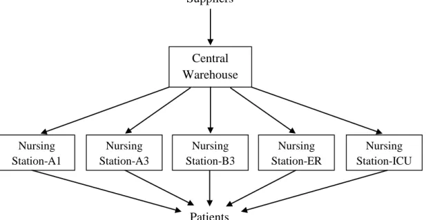
In Guven Hospital, medical supplies are controlled through a two echelon inventory system. The upper echelon is the central warehouse and the lower echelon consists of five nursing stations that are located at Block A 1st Floor, Block A 3rd Floor, Block B 3rd Floor, Emergency Room and Intense Care Unit. The corresponding inventory system can be seen at Figure 3.1.
CHAPTER 3. SYSTEM DESCRIPTION AND DATA ANALYSIS
13
Figure 3.1: Medical Supplies Inventory System in the Hospital
In this system, inventories at the central warehouse are reviewed continuously by using the inventory tracking system and orders for medical supplies are given to the related suppliers whenever necessary. The procurement department of the hospital makes contractual agreements with the suppliers. According to such contracts, shipment related costs are covered by the suppliers and the suppliers agree to deliver the items within a certain amount of time. After the arrival of the medical supplies, the warehouse personnel enters the quantities of each item to the inventory tracking system. In the central warehouse the medical supplies are stored until they are requested and retrieved for the nursing stations. The central warehouse is operating between 9:00 am and 6:00 pm. After 6:00 pm until 9:00 am next day, this warehouse is closed and there cannot be any replenishment during this period.
The nursing stations serve directly to the patients. The patients to be served by the stations can be either in-patient or out-patient. For example, Nursing Station-A3 serves in-patients while Nursing Station-ER serves mostly out-patients. All of the nursing stations can observe demand throughout the day (24-hour period), regardless of the time. Once a medical item is retrieved by a nurse for a patient need, the nurse enters that record into the system by using the item’s barcode, so that they can track
Central Warehouse Suppliers Patients Nursing Station-A1 Nursing Station-B3 Nursing Station-ER Nursing Station-ICU Nursing Station-A3
CHAPTER 3. SYSTEM DESCRIPTION AND DATA ANALYSIS
14
the remaining amount of inventory as well as the information of which item is used for which patient. Nursing stations can be replenished by the central warehouse at any time during central warehouse’s operating hours (9:00 am-6:00 pm), which we call as the “day-time”, however, replenishment is not possible during its after hours (6:00 pm-9:00 am next day), which we denote as the “night-time”. Whenever a replenishment occurs at the nursing stations, each responsible nurse enters the quantities of each item to the system and stores the items.
A porter cart is being used for the delivery of items from the central warehouse to the nursing stations. The cart has a capacity in terms of volume. The same porter serves more than one nursing station during day-time. After an order is given by a nursing station, it takes about one hour to prepare and load the medical supplies on the cart, and move these medical supplies to nursing stations. With this in mind, during the last one hour just before the night-time begins, the nursing station does not place any orders, since delivery is not possible in less than one hour and the nursing station cannot be replenished before the end of the day.
Within this thesis, we focus on the inventory control operations at the nursing stations and keep the operations at the central warehouse out of the scope. We take the nursing station at Block A 3rd Floor as the representative station, since it observes demand for the highest variety of medical supplies compared to other stations. Totally, there are 195 independent medical supplies used in this station. The analysis of the types and demand rates of these supplies will be explained in the next section.
3.2 Data Analysis
As it is mentioned in the previous section, we choose the nursing station at Block A 3rd Floor as the sample station. There are 195 different medical supplies that are used in this station. We obtained detailed demand data of these medical items for six months (April 1, 2009 - September 1, 2009). The demand data include the time of each retrieval (by the nurses) instance of an item and the amount of items per
CHAPTER 3. SYSTEM DESCRIPTION AND DATA ANALYSIS
15
retrieval. Before analyzing this data, we prune them so that the outlier data, which occur due to system failures, are removed.
First of all, we classify the items into three classes A, B and C according to total demand proportion of each item within the inventory system. The related total demand data are given in the Table A.1 in Appendix A. According to this classification, A items constitute nearly 8% of the total number of items but represents nearly 83% of the total demand in six months while B items make up 22% of the total number of items but represents nearly 15% of the total demand. C items constitute 70% of the total number of items but represents 2% of the total demand.
In Table A.1, A items average daily demand is within the range of 3 and 45. This is a wide range because the first four items in this group have much higher demand than the remaining items. The range of average daily demand for the B items is 0.17 and 3, and the rest of the items belong to the group C. Note that, the total daily demand of all items is 240 on the average. We analyze the daily demands of some fast moving items and obtain their descriptive statistics for the observed demand per day by using Minitab. In Table A.2 in Appendix A, the related statistics are given for the first 42 items. Observe that the daily demands of A items have high level of variances, and Gamma distribution turns out to be the best fitted distribution for these items’ daily demands. Some A items’ histograms with distribution fits are given in Appendix B. For the B items, none of the distributions can be fitted to the daily demands. Thus, for this group of items we accumulate the daily demands into demands per 10 days and then we fit Normal distribution to the total demand per 10 days. The C items have very low daily demands, which may be observed once in a week or even once in six months. Daily demand distribution fitting is not proper for these items. For this reason, we analyze the time between demands and find out that the best distribution which fits to the interarrival times of C items is the Exponential distribution. In other words, during a day a C item’s demand is Poisson distributed. Since C items constitute only 2% of all items and it is straightforward to set a policy under Poisson demand, we exclude these items from further analysis.
CHAPTER 3. SYSTEM DESCRIPTION AND DATA ANALYSIS
16
Next, we analyze the daily demands to see if there is a correlation between items by using Minitab. For this analysis we search for the dependency within the classes. In Table 3.1 the correlation coefficients and p-values for the most demanded 10 items from group A.
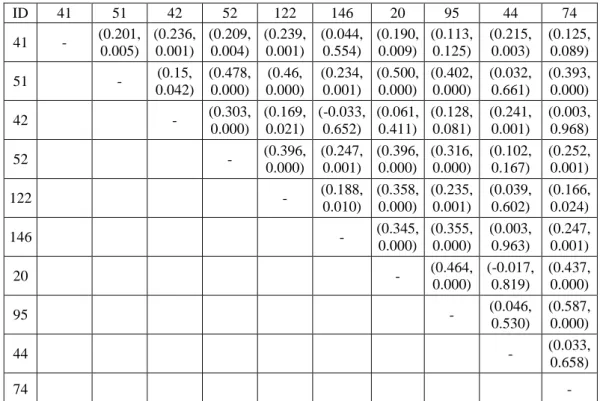
Table 3.1: Correlation analysis for A items (Correlation coefficient, p-values)
ID 41 51 42 52 122 146 20 95 44 74 41 - (0.201, 0.005) (0.236, 0.001) (0.209, 0.004) (0.239, 0.001) (0.044, 0.554) (0.190, 0.009) (0.113, 0.125) (0.215, 0.003) (0.125, 0.089) 51 - (0.15, 0.042) (0.478, 0.000) (0.46, 0.000) (0.234, 0.001) (0.500, 0.000) (0.402, 0.000) (0.032, 0.661) (0.393, 0.000) 42 - (0.303, 0.000) (0.169, 0.021) (-0.033, 0.652) (0.061, 0.411) (0.128, 0.081) (0.241, 0.001) (0.003, 0.968) 52 - (0.396, 0.000) (0.247, 0.001) (0.396, 0.000) (0.316, 0.000) (0.102, 0.167) (0.252, 0.001) 122 - (0.188, 0.010) (0.358, 0.000) (0.235, 0.001) (0.039, 0.602) (0.166, 0.024) 146 - (0.345, 0.000) (0.355, 0.000) (0.003, 0.963) (0.247, 0.001) 20 - (0.464, 0.000) (-0.017, 0.819) (0.437, 0.000) 95 - (0.046, 0.530) (0.587, 0.000) 44 - (0.033, 0.658) 74 -
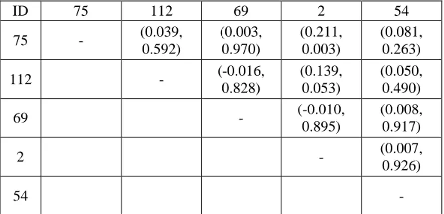
According to this table, if p-values are smaller than 0.01, then there is sufficient evidence that the correlations are not zero, otherwise the correlations between the items are zero. With this in mind, there are 28 out of 45 pairs of items which are correlated. Among these correlated pairs, the maximum absolute correlation coefficient is 0.587 and the minimum absolute correlation coefficient is 0.188. In Table 3.2 the correlation coefficients and p-values for a sample set of B items are given. Among these items, only items ID75 and ID2 are correlated with each other with a correlation coefficient of 0.211. For the C items we did not analyze the correlations, since the demand rates for those items are so low and there is no sufficient data for such analysis. Even we find out that there is a certain level of
CHAPTER 3. SYSTEM DESCRIPTION AND DATA ANALYSIS
17
correlation between some items, within this thesis we do not consider the dependencies between the medical supplies.
Table 3.2: Correlation analysis for B items (Correlation coefficient, p-values)
ID 75 112 69 2 54 75 - (0.039, 0.592) (0.003, 0.970) (0.211, 0.003) (0.081, 0.263) 112 - (-0.016, 0.828) (0.139, 0.053) (0.050, 0.490) 69 - (-0.010, 0.895) (0.008, 0.917) 2 - (0.007, 0.926) 54 -
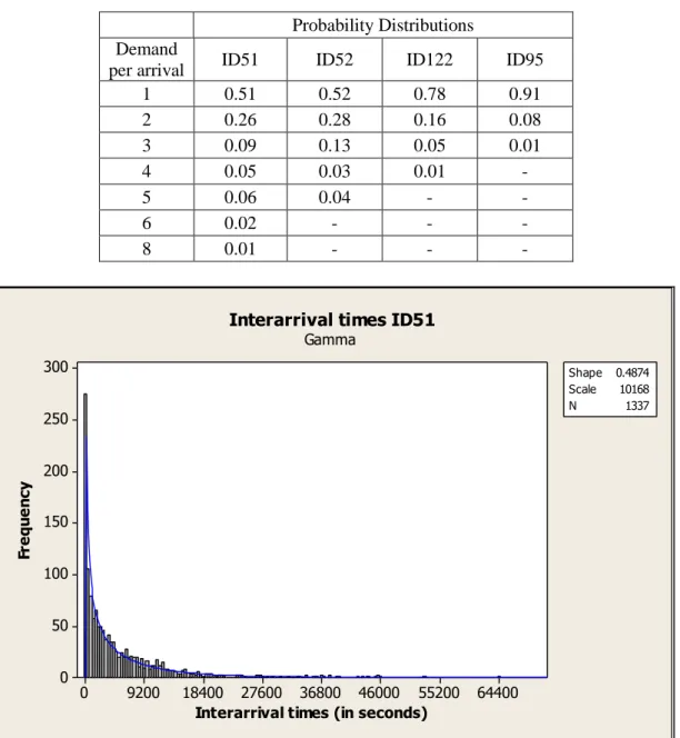
The system that we explain in the previous section makes it necessary for us to obtain distinct demand structures for the day-time and night-time. Since a continuous review policy is suitable for the day-time inventory control, we need to find the distributions for the time between demands (i.e. interarrival times) and compounding parts of these demands. On the other hand, since a periodic review policy is appropriate for the night-time inventory control, the distribution for the demand per night need to be obtained for each item. For this reason, we choose some representative items from classes A and B, and analyze their demand structure in detail by using Minitab. From Class A, we analyze the items ID51, ID52, ID122 and ID95. From Class B, we analyze the items ID75 and ID112. Note that while deciding the best fitted distribution for the related demand data, we use Minitab’s Anderson Darling test and select the distribution with the sufficiently large p-value.
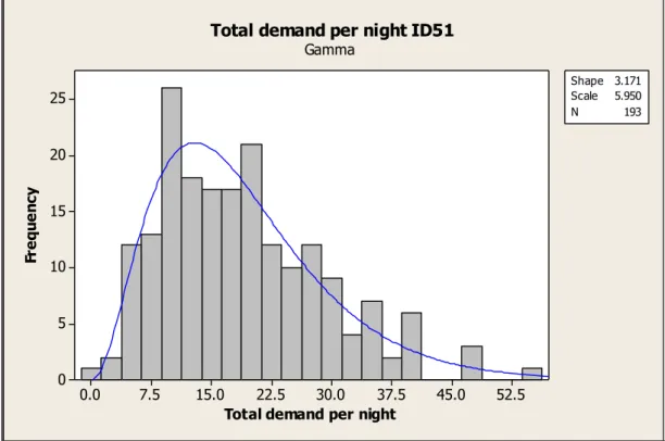
Firstly, we begin our analysis with A items. For item ID51, the interarrival times during day-time are best fitted to the Gamma distribution with shape 0.4874 and scale 10168. There is also compound part for the day-time demand of this item. We set an empirical distribution for this part as it is shown in Table 3.3. For the total demand per night the best fitted distribution that we obtain is Gamma distribution with shape 3.171 and scale 5.950. Histograms of item ID51 day-time and night-time demands with the related distributions are given in Figures 3.2 and 3.3. The distribution of the interarrival times of item ID52 is also Gamma distribution with
CHAPTER 3. SYSTEM DESCRIPTION AND DATA ANALYSIS
18
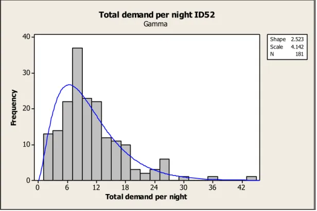
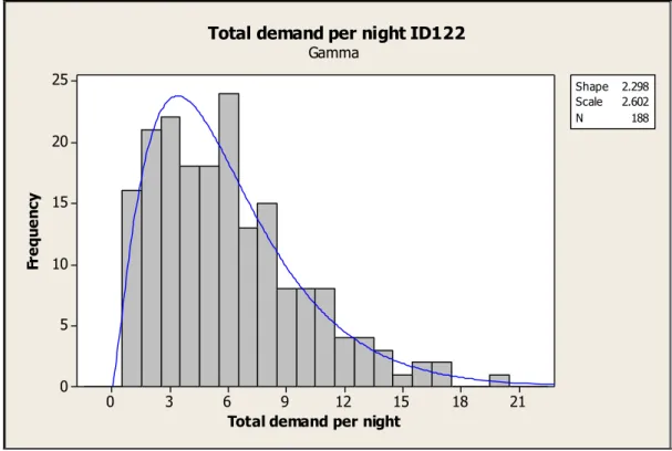
shape 0.5462 and scale 23176. Compound part of the day-time demand is shown in Table 3.3. The total demand per night is distributed with Gamma distribution with shape 2.523 and scale 4.142. Histograms with these distributions can be seen in Figures 3.4 and 3.5. The items ID122 and ID95 have also Gamma distributed interarrival times with shape parameters 0.6403 and 0.4544, and scale parameters 19437 and 34706 respectively. Demand per arrival distributions are shown in Table 3.3. The total demand per night has Gamma Distribution as well, with shape parameters 2.298 and 2.636 and scale parameters 2.602 and 1.326. These items’ histograms with the related distributions are shown in Figures 3.6, 3.7, 3.8 and 3.9.
Table 3.3: Distributions of compound parts for A items day-time demands Probability Distributions
Demand
per arrival ID51 ID52 ID122 ID95
1 0.51 0.52 0.78 0.91 2 0.26 0.28 0.16 0.08 3 0.09 0.13 0.05 0.01 4 0.05 0.03 0.01 -5 0.06 0.04 - -6 0.02 - - -8 0.01 - - -64400 55200 46000 36800 27600 18400 9200 0 300 250 200 150 100 50 0
Interarrival times (in seconds)
Fr e q u e n cy Shape 0.4874 Scale 10168 N 1337 Gamma
Interarrival times ID51
CHAPTER 3. SYSTEM DESCRIPTION AND DATA ANALYSIS 19 52.5 45.0 37.5 30.0 22.5 15.0 7.5 0.0 25 20 15 10 5 0
Total demand per night
Fr e q u e n cy Shape 3.171 Scale 5.950 N 193 Gamma
Total demand per night ID51
Figure 3.3: Histogram with Gamma fit for item ID51 total demand per night
241500 207000 172500 138000 103500 69000 34500 0 160 140 120 100 80 60 40 20 0
Interarrival times (in seconds)
Fr e q u e n cy Shape 0.5462 Scale 23176 N 578 Gamma
Interarrival times ID52
CHAPTER 3. SYSTEM DESCRIPTION AND DATA ANALYSIS 20 42 36 30 24 18 12 6 0 40 30 20 10 0
Total demand per night
Fr e q u e n cy Shape 2.523 Scale 4.142 N 181 Gamma
Total demand per night ID52
Figure 3.5: Histogram with Gamma fit for item ID52 total demand per night
80500 69000 57500 46000 34500 23000 11500 0 60 50 40 30 20 10 0
Interarrival times (in seconds)
Fr e q u e n cy Shape 0.6403 Scale 19437 N 573 Gamma
Interarrival times ID122
CHAPTER 3. SYSTEM DESCRIPTION AND DATA ANALYSIS 21 21 18 15 12 9 6 3 0 25 20 15 10 5 0
Total demand per night
Fr e q u e n cy Shape 2.298 Scale 2.602 N 188 Gamma
Total demand per night ID122
Figure 3.7: Histogram with Gamma fit for item ID122 total demand per night
218400 187200 156000 124800 93600 62400 31200 0 100 80 60 40 20 0
Interarrival times (in seconds)
Fr e q u e n cy Shape 0.4544 Scale 34706 N 518 Gamma
Interarrival times ID95
CHAPTER 3. SYSTEM DESCRIPTION AND DATA ANALYSIS 22 14 12 10 8 6 4 2 0 40 30 20 10 0
Total demand per night
Fr e q u e n cy Shape 2.636 Scale 1.326 N 166 Gamma
Total demand per night ID95
Figure 3.9: Histogram with Gamma fit for item ID95 total demand per night
Among the B items, we analyze the demand structures of the items ID75 and ID112. These items’ day-time demand interarrivals are also best fitted to the Gamma distribution with shape parameters 0.8320 and 0.5395, and scale parameters 125077 and 147852 respectively. The related histograms can be seen in Figures 3.10 and 3.11. The demand structures of these items also include compound parts, whose empirical distributions are shown in Table 3.4. The total demands per night distributions for these items are fitted to the empirical distributions as well. In Table 3.5 the probabilities of observing certain amounts of demand at each night are given.
Table 3.4: Distributions of compound parts for B items day-time demands Probability
Distributions Demand
per arrival ID75 ID112
1 0.88 0.93
2 0.10 0.06
3 0.02 -
CHAPTER 3. SYSTEM DESCRIPTION AND DATA ANALYSIS 23 560000 480000 400000 320000 240000 160000 80000 0 10 8 6 4 2 0
Interarrival times (in seconds)
Fr e q u e n cy Shape 0.8320 Scale 125077 N 91 Gamma
Interarrival times ID75
Figure 3.10: Histogram with Gamma fit for interarrival times of item ID75
504000 432000 360000 288000 216000 144000 72000 0 20 15 10 5 0
Interarrival times (in seconds)
Fr e q u e n cy Shape 0.5395 Scale 147852 N 89 Gamma
Interarrival times ID112
CHAPTER 3. SYSTEM DESCRIPTION AND DATA ANALYSIS
24
Table 3.5: Distributions of night-time demands for B items Probability
Distributions Demand
per night ID75 ID112
0 0.71 0.61 1 0.18 0.32 2 0.07 0.06 3 0.01 0.01 4 0.01 -6 0.01 -10 0.01
-To sum up, in this Chapter we analyze the six months transaction data of the nursing station at Block A 3rd Floor. We classify the items into three classes according to total demand proportion of each item within the inventory system. Then, after obtaining the total daily transaction of each item, we find the daily demand distributions, which can be either a known distribution or an empirical distribution, whichever fits the best. Moreover, in order to use in the numerical analysis in Chapter 5, we obtain the best fitted distribution for the interarrival times during the day-time (i.e. time between each transaction during a day). For each item, we find the distribution of total demand per night for using in the numerical analysis. For this analysis, we also find the distribution of the compounding part of demand for each item (i.e. number of items retrieved in each transaction).
25
Chapter 4
Model and Policies
4.1 Definition of the Inventory Problem
We consider a multi-item two echelon inventory system where the upper echelon is a central warehouse and the lower echelon involves smaller depots which are nursing stations. We assume an ample supply at the central warehouse which is capable of meeting the demand of nursing stations whenever necessary. The central warehouse operates during a certain period of time of any given day, and is closed during the remaining times. Due to such on- and off-periods of the central warehouse, it is possible to replenish the nursing stations during the day-time on a continuous scale but it is not possible to make any replenishment during the night-time.
In our setting, satisfying target service levels (i.e. fill rates) is the prior performance measure rather than the cost measure, while making inventory control decisions. Note that this priority is the natural choice for hospital operations. Nevertheless, we still aim to minimize average inventory levels, because of the capacity of the nursing stations and the inevitable cost considerations. In other words, we want to make sure
CHAPTER 4. MODEL AND POLICIES
26
that the average proportion of demand that cannot be met during day-time and night-time should be less than a specified level with minimum average inventory levels.
During the first time frame (day-time), demand can be observed at anytime and a capacitated cart is used for moving the items from upper echelon (the central warehouse) to the lower echelon (nursing stations) whenever a replenishment occurs. We denote the replenishment lead time by which starts at the time that an order is given until it is received by the nursing station.
During the second time frame (night-time), demand can still be observed at anytime at the nursing stations. However, the upper echelon is closed during this time frame and for this reason replenishment cannot take place. This particular situation makes it necessary to treat the day-time and night-time demand separately. Since replenishment is possible at anytime during the day-time and achieving high service levels targets is the main concern, controlling inventory at a continuous basis during the day-time would be the most logical choice. However, since replenishment is not possible during the night-time, the inventory control for this time period can only be made at a periodic basis. In particular, a one time decision is made for the whole night every day. Consequently, the day-time and night-time demands should be modeled and handled differently. We assume a compound renewal type demand, i.e. the interarrival times of the demand instances and compounding demand per arrival are both random variables, for the day-time. On the other hand, the whole night-time demand, which is also a random variable, is denoted by a single probability mass distribution.
Consider a 24-hour period starting at some time . This starting time, , also marks the start of the first time frame (day-time). The first time frame ends at time which also marks the start of the second time frame (night-time). This second time frame ends at time of the next 24-hour period. Let be the random variable denoting the compounding part of the demand observed at a demand instance during day-time, be the random variable denoting the interarrival times of the demand during
day-CHAPTER 4. MODEL AND POLICIES
27
time, and be the random variable denoting the accumulated total night-time demand between and .
Figure 4.1: Demand structure
Within the scope of our problem, we assume that the medical supplies are independent of each other. Note also that the total demand during night-time is always greater than or equal to the total demand observed during lead time for each medical supply in our particular context. Considering these assumptions and the demand structure illustrated in Figure 4.1, we aim to find an appropriate inventory control policy, which leads high service levels for both day-time and night-time demand, while minimizing the average inventory levels.
4.2 Solution Approaches
Having two structurally different demand streams, as day-time and night-time demands, yields a different inventory control problem than the typical ones. One possible approach for this situation could be to obtain a non-stationary single demand distribution by interlacing these two demand streams and search for the optimal inventory control policies accordingly. By using this aggregated distribution, we may find the optimal inventory control policies for this system; nevertheless, this approach involves difficulties in terms of analyzing the system itself, since the resulting distribution will have a time-dependent non-stationary structure. In this thesis, we aim to find policies which are easy-to-implement and whose parameters are easy to find for each medical supply.
Day 2 Day 1 a n d e n d a t a n d e n d a t a n d e n d a t
CHAPTER 4. MODEL AND POLICIES
28
4.2.1 Our Proposed Control Policy
In our system, using a stationary inventory control policy with same parameters for day-time and night-time is not an appropriate way to satisfy the high service levels with low inventory levels. Because, this may cause high inventory levels during the day-time in order to meet the night-time demand or on the contrary it may lead to lower inventory levels but at the same time it may cause failure to satisfy the high service levels during night-time. Thus, separate control policies or same policy with different parameters for day-time and night-time demand can be used in order to make sure that our operational targets are satisfied.
In order to take action before observing stockout at the medical supplies during day-time, continuous review policies would be appropriate. Among the continuous review policies, we search for the ones that are suitable for environments where high service levels are required and a limit on the order size is imposed. For this reason, policies which only consider high service levels but do not take limit on the order size into account, such as and are eliminated (Tanrikulu et. al., 2009). Since and policies take the capacity and utilization of that cart into account, we take these policies as the candidate policies. The policy employs a fixed order amount at each replenishment. Nevertheless, as it is mentioned by Tanrikulu et. al. (2009), it does not take each item’s inventory levels into consideration; instead under this policy replenishment is made when the total demand of all items reaches . Therefore, this policy cannot respond quickly, if one item’s inventory level drops below zero, before the total consumption reaches . Another policy, which utilizes a constant order at each replenishment, is the policy. This policy can also satisfy high service levels without carrying excess amount of inventory. Tanrikulu et. al. (2009) points out that this policy outperforms policy especially when the high service levels are required and lead times are low. This comparison fits exactly our case when we think backorder costs as service level requirements in our problem.
CHAPTER 4. MODEL AND POLICIES
29
Consequently, we propose policy to be used for day-time inventory control. Under this policy, inventory positions of all items are reviewed continuously and when one item’s inventory position drops to its reorder point , a fixed order is given. In this joint order, each item’s order size is determined by a heuristic allocation method, which is also used by Tanrikulu et.al. (2009), with the aim of balancing each item’s inventory position in excess of the reorder point. Let be the inventory position of item at any time and be the reorder level of item . By using this allocation method, each item’s inventory position ( ) is brought above its reorder level ( ). Moreover, since we use a capacitated cart for the replenishment and we want it to be fully utilized, we allocate the remaining amount of in a way that we balance each item’s inventory position in excess of its reorder level. We allow for ordering more than one if it is necessary at an ordering instance. With this in mind, our proposed allocation method is given below.
for if else end while = end
In order to satisfy the night-time demand, there is no need to hold inventory in advance throughout the day-time, but giving an order, just one lead time before the night-time starts would be sufficient. Thus, we suggest a periodic review policy for night-time inventory control. In other words if the replenishment lead time is one
CHAPTER 4. MODEL AND POLICIES
30
hour, then controlling the inventory level and giving order if necessary at will be appropriate for both satisfying night-time service levels and holding less inventory. For the night-time inventory control, we propose policy, where . By using this policy for the night-time demand, the necessary amount of order, that is required to bring inventory positions up to each item’s , is given just a lead time before the night-time demand is observed. Thus, without holding inventory for a long time, high service levels can be satisfied for the night-time.
To sum up, we propose a hybrid policy, which involves continuous review policy for the day-time demand and periodic review policy for the night-time demand. Note that, in the multiple items case, of the policy and of the policy are vectors of numbers corresponding to the reorder and order-up-to points of items respectively. In the remainder, we do not include an index for items for brevity but we note that each expression is valid for each item. In Chapter 5, we will show how we can find the exact or estimated policy parameters for this hybrid policy in order to satisfy the specified service levels.
4.2.2 A Special Case: Single-Item
In this section, we analyze a special case of our system: the single-item case. We explain our approach for an item observing renewal type individual demand but this approach can also be extended to compound demand situations. We develop exact expressions that can be used to calculate different performance measures such as total expected cost, service levels, etc. When there is only one item in the system, then the proposed policy becomes the well known policy. In this special case, we treat the night-time demand in the same way as it is in the multi-item case, hence we suggest policy to be used for the night-time inventory control. Summary of the notation used in the remainder is given in Table 4.1.
CHAPTER 4. MODEL AND POLICIES
31
Table 4.1: Notation
As explained in the previous section, at time , the inventory position of the item is raised up to . Due to the nature of the system, no orders are placed during and all outstanding orders at time would arrive until time . Therefore, the inventory level at time before the night-time demand is observed, , is given by . Afterwards, the total demand for night-time is observed which causes the inventory level at to drop to the value and next day’s starting inventory position to take the value which is equal to before any order is given in the next day as shown at Figures 4.2a and 4.2b. We analyze two possible scenarios where the actions taken at time are different. In Figure 4.2a observed night-time demand is so low that the beginning inventory position is greater than the reorder point ( ) and for this reason no order is given at the beginning of the next day.
: Reorder point for the day-time replenishment : Fixed order amount for the day-time replenishment : Periodic review instance for the night-time replenishment : Order up to level for the night-time replenishment
: Replenishment lead time : The start of the day-time : The start of the night-time
: Random variable denoting the demand during lead time : Random variable denoting the demand during night : Amount of demand observed by time
: Inventory position at time : Inventory level at time
: Inventory level at time after the order arrives for the night and before the night’s demand is observed
i.e.
: Inventory level at time after the order arrives for the night and night’s demand is observed
CHAPTER 4. MODEL AND POLICIES
32 r
Figure 4.2a: First example for the behavior of inventory level over time
Figure 4.2b: Second example for the behavior of inventory level over time Inventory Level Time: t : : Inventory Level Time: t : : r r
CHAPTER 4. MODEL AND POLICIES
33
On the other hand, in Figure 4.2b total demand observed during night-time is high enough that the inventory position at the beginning of the day ( ) drops below the reorder point ( ) and an order is given at , in order to bring the inventory position to or over . After the ordering is made at time , the inventory position will take a value between and . After this, regular policy is implemented until time at which the inventory position is raised to again for the following night-time.
Rather than modeling this particular inventory system as a whole on an infinite horizon continuous time scale, we model the inventory system for every “day-time” (the time range from to ) separately, where the policy is employed on a continuous time scale. Note that each “day-time” is stochastically equivalent to each other. In this model, we also explicitly consider the effect of the policy. We first develop exact expressions to estimate the probability distributions of the inventory position at any given time where by using a transient analysis, and then this information is used to find the probability distributions of the inventory levels at any time .
When the system is controlled by the policy, takes a value between and . A typical inventory system operated with the policy can be modeled as continuous time Markov Chain by defining the states of the system as the inventory position. Let for some time . Whenever a demand arrival occurs after time , the system will move to the state if and to the state if . Suppose that at a given time and for some such that . Then the probability that is equal to at another given time and for some such that , is the probability that there are or or or ... demand arrivals during the time interval . Similarly, the probability that is equal to for some , is the probability that there are or or ... demand arrivals during the time interval .
CHAPTER 4. MODEL AND POLICIES 34 . . . 2 2 2 2 2 1 1 ... ... 2 2 2 3 3 3 3 3 3 3 3
The case for is illustrated in Figure 4.3. In this figure, the nodes represent the inventory positions during the time interval . After starting at , in order to end at the first possibility for the total demand arrivals during , is , and is shown by the arcs, which are marked as “1”. As the second possibility, the total demand may be equal to and this situation can be obtained by starting with arcs “1” and continue with one full cycle by using arcs “2”. The third possibility, which is , is shown by the arcs “1”+“2”+“3”, in other words this possibility consists of arcs “1” followed by two full cycles.
Figure 4.3: Illustration of the demand arrivals within for
The boundary conditions (initial conditions) for this model is given by the probability distribution of the inventory position at time , i.e. . The starting point of each day-time interval is and can be obtained as follows. By conditioning on the smallest number of orders that can bring the inventory position at the beginning of the day to or over the value , can be found.
if then we do not give any order ... . . . . . . . . . . . . . . . . . . . . .
CHAPTER 4. MODEL AND POLICIES 35 if if then we order Q if then order 2Q if then order 3Q
We can generalize this structure where = (4.1) (4.2)
By substituting Equation (4.1) into (4.2), we obtain:
(4.3)
By using this information and the above discussion, we can calculate the inventory position of the item at any given time as follows.
For the case when we drive the equations as follows:
CHAPTER 4. MODEL AND POLICIES 36 Assume ... Assume ...
We can generalize these expressions for where and as:
. (4.5)
For the case when the structure of is different than the previous case. Assume ...
CHAPTER 4. MODEL AND POLICIES 37 Assume ...
We generalize these expressions for . For and :
. (4.6)
For and :
. (4.7)
Actually, since for any distribution we can modify the interval for in Equation (4.7) as .
In general, Equations (4.1)-(4.4) can be combined and rewritten as:
for and
for and (4.8)
Now we can find by using Equation (4.8) conditioning on as follows: