Hopf bifurcation in an overlapping generations resource economy with endogenous population growth rate

Burcu Fazlıoğlu, Hüseyin Çağrı Sağlam and Mustafa Kerem Yüksel*

Hopf bifurcation in an overlapping

generations resource economy with

endogenous population growth rate

Abstract: As scarce environmental resources necessarily put a constraint on population growth, we use more realistic population growth dynamics which contemplates a feedback mechanism between population growth rate and resource availability. We examine the local stability properties in overlapping generations resource economies which takes this feedback mechanism into account. The results indicate that Hopf bifur-cation may arise without requiring logistic regeneration or unconventional constraints on parameter values. In particular, Hopf bifurcation is encountered under convex-concave dependence of carrying capacity on the resource availability.

Keywords: endogenous population growth; hopf bifurcation; overlapping generations model; renewable resource.

JEL Classification: D90; Q20; J10; C6.

1 Introduction

In response to a feedback mechanism between population growth and carrying capacity of the environment, scarce environmental resources have been advocated to put a constraint on population growth (Smith 1974). Indeed, Smith (1974) postulates that population growth should possess the following properties for a more realistic growth model: “1) when population is small in proportion to environmental carrying capacity, then it grows at a positive constant rate, 2) when population is large in proportion to environmental carrying capac-ity, the resources become relatively more scarce and as result this must affect the population growth rate negatively” (see Accinelli and Brida 2005; Brianzoni, Mammana, and Michetti 2007, 2).

Motivated by Smith’s idea, we analyze the dynamics of an overlapping generations economy that contemplates a feedback mechanism between population growth rate and resource availability. We adopt a Beverton Holt population growth function (see Beverton and Holt 1957) which is a discrete time version of the logistic population growth function (for the logistic population growth function see among others, Schtickzelle and Verhulst 1981; Faria 2004; Accinelli and Brida 2005; for a discrete time Romer model, see Brianzoni, Mammana, and Michetti 2007). However, we modify Beverton Holt population growth function in which the carrying capacity is a convex-concave function of the available resource stock. As carrying capacity of nature are nor fixed neither static (Arrow et al. 1995), we consider that the carrying capacity increases with the available resource stock at an increasing rate at first and at a decreasing rate afterwards. This is simply more realistic because population growth rate responds to the changes in the available resource stock and population is bounded from above. Through this feedback mechanism between population and resource

*Corresponding author: Mustafa Kerem Yüksel, Department of International Trade and Finance – University of Turkish Aeronautical

Association, Ankara, Turkey; and Department of Economics – Bilkent University, Ankara, Turkey, e-mail: mkerem@bilkent.edu.tr

Burcu Fazlıoğlu: Department of International Entrepreneurship – TOBB ETU University, Ankara, Turkey Hüseyin Çağrı Sağlam: Department of Economics – Bilkent University, Ankara, Turkey

availability, we show that the introduction of endogenous population growth rate implies that Hopf bifurca-tion may emerge in an overlapping generabifurca-tions resource economy.1

Nonlinear dynamics (such as multiplicity of the steady states or Hopf bifurcation) have been obtained in overlapping generations models with resources (see among others Koskela, Ollikainen, and Puhakka 2008; Antoci and Sodini 2009). The dynamics in these studies mainly rest on the assumptions of logistic regeneration function or some assumptions on the intertemporal elasticity of substitution.2 _{Under logistic} regeneration function of resources, it has been shown that further assumptions on the parameters of utility and production function bring dynamics such as local indeterminacy or bifurcations. In particular, Koskela, Ollikainen, and Puhakka (2008) examine whether renewable resource based overlapping generations econo-mies may have different types of dynamics other than saddles. They demonstrate that flip bifurcation may arise under inefficient equilibrium. They numerically assign the value one to the intertemporal elasticity of substitution in consumption to obtain a subcritical flip bifurcation. Our setting allows us to obtain Hopf bifurcation under the convex-concave dependence of carrying capacity on the resource availability without referring to logistic regeneration, shocks or constraints on parameter values. Thus, the novel feature of our study is to reveal Hopf bifurcation by incorporating endogenous population growth rate à la Smith (1974). In this regard, our study complements Koskela, Ollikainen, and Puhakka (2008), Seegmuller and Verchère (2007) (overlapping generations economy with environment and endogenous labor supply) and Antoci and Sodini (2009) (an overlapping generations economy with negative environmental externalities) that provide additional channels for interesting dynamics in overlapping generations framework.

The paper is structured as follows. The model is introduced in the following section. The equilibrium dynamics and the local stability analysis are provided in Section 3. Section 4 concludes.

2 The model

We consider a two period overlapping generations model with infinite horizon. We differ from the standard framework in two respects.3 _{Firstly, we assume that the renewable resources are essential to production.} Second, under the presence of limited resources, we allow for the growth rate of the population to depend on the per capita resource availability.

At each period t, a generation of agents appears and lives for two periods, young and old. The population in period t, consists of N_t young and N_t-1 old individuals. We assume that the rate of population growth n_t+1 is related with the total available resource stock E_t, and the population growth rate n_t:

+1= +(1 ) , t t t N n N where +1= ( , ) and = t. t t t t t t E n g e n n e N

We consider a Beverton-Holt population growth rate function (see Beverton and Holt 1957) in which the carrying capacity of the environment depends on the available per capita resource, ,e stock in the following _t

manner:

1 Hopf bifurcation is economically important as it provides a powerful and easy tool to detect limit cycles and justify the

emer-gence of cycles endogenously (for further details, see Benhabib and Farmer 1999; Kind 1999).

2 Under linear regeneration of renewable resources, the overwhelming majority of standard resource models in OLG framework

(where population is constant or growing at a consant rate, see Kemp and Van Long 1979; Farmer 2000; Valente 2008) reveal that the dynamics converge to a single steady state or to a balanced growth path with saddle path stability (see Mourmouras 1991).

= + − ( ) ( , ) , ( ) ( 1)t t t t t rh e g e n h e r n

where h(e): ℝ+_→ℝ+ _{represents carrying capacity of the environment and r > 1 denotes inherent growth rate (this} rate being determined by life cycle and demographic properties such as birth rates, etc., see among others, Brianzoni, Mammana, and Michetti 2007). We conjecture that for low values of the resource stock the carry-ing capacity of the environment increases with an increascarry-ing rate while for high levels of the resource stock at an increasing rate at first and at a decreasing rate afterwards with the following convex-concave function (Capasso, Engbers, and Torre 2012):

ρ ρ τ τ = +1₂ ( ) , 1 e h e e (1)

with τ₁ > 0, being population scale factor, τ₂, ρ > 0 being population curvature parameters.4

The resource can act as both stores of value and inputs to the production process. The economy is initially endowed with a positive amount of the natural resource E₀ which belongs to the first generation of old agents. We assume that at the beginning of each period t, the old agents (generation t–1) own the stock of the natural resource, E_t. Incurring no extraction costs (see Dasgupta and Heal 1979), old agents decide on how much of this resource will be extracted for production X_t and how much would be sold to the young (generation t) as assets A_t( = E_t–X_t). From period t to t+1, the assets bought by the young generation regenerate at a rate Π ≥ 1.5 Therefore, the law of motion of the resource stock writes as follows:

Π Π + + = = − + = − 1 1 , , (1 ) ( ), t t t t t t t t t E A a e x n e e x

where quantities of resource assets and extracted resources per young individual are denoted by, = t, = t t t t t E A e _N a _N and = ,t t t X x N respectively.

Each agent is endowed with one unit of labor when she is young and supplies it to firms inelastically. Young households receive wage w_t, which is allocated between consumption of the good produced by the rep-resentative firm and the purchase of the ownership rights for the natural resource. When old, they consume their entire income generated by selling their stock of natural resources X_t+1 to the firms and their assets A_t+1 to the young at prices P_t+1 and Q_t+1, respectively. We assume that the life-time well-being of the representa-tive individual is measured by the logarithmic function over young and old periods consumption, i.e. U(c_t,

d_t+1) = u(c_t)+βu(d_t+1), where β∈(0, 1) is the subjective discount factor. Accordingly, the representative agent born in period t, maximizes his utility with respect to the young and old periods’ consumption, taking wages and the price of the natural resource as given.

4 Note that ρ ρ τ ρ − = + 2 1 ( 1)

e determines the inflection point at which carrying capacity h(e) function switches from convexity to concavity, or vice versa (this point is simply the one through which the second derivative changes sign). Also note that for the parameter combination (τ2, ρ), e is on the convex portion of the function if it satisfies ρ

ρ τ ρ − < +

2 _{( 1)e}1 ; and e is on the concave portion

of the function if it satisfies ρ

ρ τ ρ − > +

2 _{( 1)e}1 . The second derivative of h(e) with respect to e is ρ ρ ρ τ ρ ρ τ ρ τ − _{− − +} = + 2 2 1 2 2 3 2 [ 1 ( 1)] ( ) _. (1 ) e e d h e de e

β +1 + +1 { ,c d amax ln t t , }t ct ln dt subject to + = , t t t t c Q a w (2) +1= +1(1+ ) +1+ +1(1+ ) ,+1 t t t t t t t d P n x Q n a (3) Π + + ₁= (1 n e_t) _t a (4)_t, + + = − ≥ ≥ ≥ 1 1 0 , 0, 0, 0, >0, given. t t t t t t a e x c d e E (5)

The first order conditions for an interior solution of this problem is as follows: Π β +1₌ +1_, t t t t d Q c Q (6) +1= +1. t t P Q (7)

Firms are owned by the old households and produce an homogenous consumption good under perfect competition. At each period, a single final good Y_t is produced in the economy by means of labor L_t and the natural resource X_t according to the following technology:

α −α _α

= 1 _{, 0}< <_1.

t t t

Y X L

Under the perfectly competitive environment, the representative firm producing at period t maximizes its profit by choosing the amount of labor L_t and the resource input X_t that will be utilized in the production process. At an interior solution of the firm’s optimization problem, where all variables are expressed in per capita terms _ = _

 t t,

t

Y y

L profit maximization implies:

α

− =

(1 )y w (8)_{t t},

α =y P x (9)_{t t t}.

Intertemporal equilibrium requires the clearing of the resource market, the clearing of the labor market and the clearing of the goods market for all t:

Π + + ₁= − (1 n e_t) _t (e x _{t t}), (10) = _, t t L N (11) − − = + + 1 1 (1 ) . t t t t y c d n (12)

3 Equilibrium dynamics

The intertemporal equilibrium dynamics can be reduced to a three–dimensional linear system in terms of the law of motions of e_t, x_t and n_t.

From equations (2)–(8) and (12), we obtain that α β β − = = + (1 ) ,+ (1 ) (1 )t t t w y c (13)

α β β + + + + = + 1 1 (1 )( ) _. (1 )t t t n d y (14)

Plugging equations (7), (9), (13) and (14) into (6), we obtain the law of motion of the resource stock:

Πβ α α β + − = + + 1 (1 ) _. (1 )( ) t t t x x n (15)

In addition, we have the dynamics of the natural resource stock and the population:

Π Π +1=−₍₁₊ t_{) (1}+ ₊ t₎, t t t x e e _{n n} (16) +1= ( , ) . t t t t n g e n n (17)

Thus, the dynamics of the model economy is driven by (15), (16) and (17).

Lemma 1 (Steady State Equations) The steady states are characterized by the following equations:

Πβ α α β  − _{− =}  _{+ +}  (1 )((1 ) 1 0,)  x _n (18) ( , 1 ) 1, (1 ) 0 ( ) s n o that x or Πβ α α β − ₌ + + = Π Π  ₋  ₌   (1 )+n 1e (1 )+n x, (19) − = ( ( , ) 1) 0, n g e n (20) = = , 0 ( , ) 1. so that n or g e n

The Jacobian that governs this system of equations at the corresponding steady states is as follows:

( )

Lemma 2 (Locally Unique Steady States) Among the steady states characterized by equations (18), (19) and (20), the following are the ones that satisfy local uniqueness:

1. Zero Steady State with Zero Population Growth with x = e = n = 0;

2. Zero Steady State with Non-zero Population Growth with x = e = 0, g(0, n) = 1 and g(0, 0)≠1; 3. Non-zero Steady State with Zero Extraction with x = 0, Π =₊ 1,

(1 )n and g(e, n) = 1;

4. Non-zero Steady State with Non-zero Extraction with Πβ α α β − ₌ + (1 ) 1,+ (1 )(n ) Π Π  ₋ ₌  ₊  ₊ (1 )n 1e (1 )n x, and g(e, n) = 1.

Zero Steady State with Zero Population Growth (i.e. first steady state) and Zero Steady State with Non-zero Population Growth (i.e. second steady state) exhibit monotone dynamics since the associated eigenvalues are

all positive and real. Non-zero steady states constitute a more interesting case than that of the zero steady states. However, those steady states exhibit nonlinear dynamics under plausible parameters. In what follows we will concentrate on the emerging of Hopf cycles around these steady states.

The analysis of Hopf bifurcation provides a powerful and easy tool to detect limit cycles that discard tedious calculations. Hopf cycles appear when a fixed point loses or gains stability due to a change in a parameter and meanwhile a cycle either emerges from or collapses into the fixed point. The dynamic system can either have a stable fixed point surrounded by an unstable cycle; or a stable cycle loses its stability and a stable cycle appears as the parameter(s) approach(es) to a critical value (see Asea and Zak 1999; Yüksel 2011). Both cases can be economically significant (for further details see Kind 1999).

3.1 Hopf bifurcation at the non-zero steady state with zero extraction

Non-zero Steady State with zero Extraction exhibits Hopf bifurcation for specific parameter combinations and

to prove the result, we need the following lemma.

Lemma 3 (Hopf Conditions for 2 × 2 discrete dynamic system) Let J be a 2 × 2 Jacobian matrix associated with

the 2 × 2 discrete dynamic system and T and D be the trace and the determinant, respectively. Then, Hopf bifurca-tion occurs when

= − < < 1, 2 2. D T

Proof. See Antoci and Sodini (2009, 1443). ■

Proposition 1 Consider the following modified Beverton-Holt specification, =

+ − ( ) ( , ) _{( ) ( 1)}t , t t t rh e g e n _{h e r n} with r > 1

and a convex-concave carrying capacity ρρ

τ τ = +1₂ ( ) 1 e h e

e with ρ, τ1, τ2 > 0. If there exists a parameter combination (Π, r, ρ, τ₁, τ₂) such that Π = + ′ > ( ) 1 , 1, h e e n

then the Non-zero Steady State with Zero Extraction,

Π

=0, = −1, = ( ),

x n and n h e

undergoes a Hopf bifurcation.

Proof. The Jacobian associated with this steady state is

β α α β Π  −   ₊    _{− −}   _{+ +}   ₊      (1 ) 0 0 ( ) 1 . (1 ) (1 ) 0 _{e n} 1 e n n g n g n

β α λ λ λ α β  _{− −}   _{− − − +} ₌    _{+   + } ((1 ))  ( 1)( g nn 1) (1 )e_n nge 0,

reveals that one of the eigenvalues is λ β α α β − =

+

1 ₍(1 )._{) Note that} λ1 < 1. Then, if the remaining second order polynomial has complex roots with unit magnitude, we can conclude that the steady state exhibits Hopf bifurcation (see Wen et al. 2002). Consider, the 2 × 2 matrix associated the quadratic polynomial,

 ₋   ₊    +     1 _. (1 ) 1 e n e n ng g n (21) Denote = + = + + ₊ 2 , 1 , (1 ) n n e T g n e D g n ng n

as the trace and the determinant of matrix (21), respectively. Rewriting the Hopf conditions (see Lemma 3), we have

< =− <

+

0 4.

(1 )e ng g n_n e n (22)

From the steady state condition (20), we know that g(e, n) = 1. Since = + − ( ) ₁ ( ) ( 1)rh e h e r n and r > 1, we have = ( ) . h e n (23)

From (1), (23) and the fact that h′(e) = 1+n, the steady state can be recast as,

ρ ρ Π τ τ = = − > = +1₂ 0, 1 0, . 1 x n e _n e

Now, we want to show that this steady state satisfies the Hopf conditions provided in (22). Note that, − ′ = + − − − = + − 2 2 ( )( 1) , [ ( ) ( 1) ] ( )( 1) . [ ( ) ( 1) )] e n rh e r n g h e r n rh e r g h e r n

Furthermore, note that,

− =− = + 1, (1 )e_n nge g nn r_r and we need, − < 1< < 0 r_r 1 4. Note that since r > 1, 0<r−1<4

r is already satisfied and casts no restriction on the parameters and especially

on r itself.

We further provide an exemplary set of parameters that yields Hopf bifurcation. Example 1 Consider the following benchmark parametrization,

ρ=3, τ₁=1, τ₂=0.05, 0.33, 0.98,α= β=

and further assume that

Π =_bif 1.5203.

Then, the steady state

Π −

=_0, = − =_{1 0.5203,} = 1_{( ) 0.8114,}=

x n and e h n

undergoes Hopf bifurcation for every r > 1.

The above example clearly shows that there exists Hopf bifurcation for plausible parameters. However, to fully comprehend the relationship of the parameters which causes Hopf bifurcation, we further our analysis by constructing a Hopf boundary.

For any r > 1, trace of the Jacobian satisfies,

− − < < = −2 1 T 2 r_r1<2.

Thus, by Lemma 3, Hopf condition reduces to D = 1. Given the steady state equations, the determinant of the Jacobian in terms of ρ and Π is

ρ Π τ Π τ ρ Π τ Π    −  − − − = +_  _{ } 1 2 − _ 1 ( 1)( ( 1) ) 1 1 ( , ) r 1 . D r r

Given that r > 1, (ρ, Π) couples that maintain the condition that D(ρ, Π) = 1 imply that 1 Hopf 1 2 . ( 1)( ( 1) ) τ Π ρ Π τ Π τ = − − − (24)

Equation (24) gives the Hopf boundary. Figure 1 depicts the complex eigenvalues boundary (dashed curve) and Hopf boundary (solid curve). In detail, for the (Π, ρ) couples that lie in the upper contour set of the dashed curve, the resulting eigenvalues are complex. For the (Π, ρ) couples that lie in the upper [lower] contour set of the solid curve, the resulting (complex) eigenvalues are outside [inside] the unit circle [i.e. their magnitude is higher (smaller) than 1]. In other words, when (Π, ρ) falls into the upper contour set of the Hopf boundary, one has two unstable (complex) and one stable (real) eigenvalue (saddle path solution). When (Π, ρ) falls between the Hopf boundary and complex eigenvalues boundary, one has two stable (complex) and one stable (real) eigenvalue (indeterminacy). For the (Π, ρ) couples on the Hopf boundary, an infinitesimal change in the parameters forces complex eigenvalues cross the unit circle (loss or gain of stability) Thus, as the parameters (ρ, Π) vary, we observe Hopf bifurcation.6

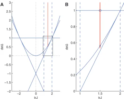
In Figure 2, we present the trace-determinant space for a second order characteristic equation.7 _{Note that} trace only depends on r, thus as parameters (ρ, Π) vary, trace stays constant. This can be clearly seen in the 6 Note that Π > 1 by definition and τ

τ Π< + 1

2

1 to ensure a positive value for ρ.

7 The trace-determinant space is a standard graphical procedure to evaluate the roots of a second order characteristic equation

(For further details see among others, Grandmont and Laroque 1990, 83; Azariadis 1993, 62–67, 93; Grandmont, Pintus, and de Vilder 1998). The idea is tractable and simple: Evaluated at the steady state, if the trace-determinant of the Jacobian falls above the parabola, the resulting eigenvalues are complex; and inside the triangle, they are fully stable. To identify bifurcations, it is sufficient to trace the trace-determinant couple and check whether the couple crosses certain borders. Hopf bifurcation boundary is identified as the portion of the horizontal det J = 1 line that stays above the parabola.

line in Figure 2 which is obtained when r = 2, without loss of generality. In Figure 2, Π = 1.5203 is kept constant and as ρ varies, one can keep track of the determinant. For the small values of ρ, the trace-determinant couple stays in the stable region (triangle) where the eigenvalues are real. As ρ increases and exceeds,

τ Π ρ Π τ Π τ  −  = _ _{ − − −}1 = complex 1 2 1 1 _0.375, 4 rr ( 1)( ( 1) ) 0 5 10 15 20 0 2 4 6 8 10 12 14 16 18 20 Π ρ A 1 1.5 2 0 0.5 1 1.5 2 2.5 3 3.5 4 Π ρ B

Figure 1: (A) Π–ρ couples at which the complex eigenvalues (dashed) and Hopf bifurcation (solid) occur (τ1 = 1, τ2 = 0.05) (B) A

closer look [rectangle in part(a)]. Π = 1.5203, fixed. Solid line traces the ρ values starting from 0.2. At ρ = 0.375 (at  × ), complex eigenvalues emerge. At ρ = 3 (at +), complex eigenvalues cross the Hopf boundary.

–2 0 2 –2 –1.5 –1 –0.5 0 0.5 1 1.5 2 2.5 3 trJ det J A 1 1.5 2 0 0.2 0.4 0.6 0.8 1 trJ det J B

Figure 2: (A) Trace-determinant space for a second order characteristic equation. Inside the triangle, fully stable, above the

parabola complex eigenvalues. Trace is solely determined by r and is between 1 and 2 (dashed lines). Π = 1.5203, fixed. Vertical solid line traces the tr-det values with respect to ρ∈(0.2, 15). (B) A closer look [rectangle in part(a)]. At ρ = 0.375 (at  × ), complex eigenvalues emerge. At ρ = 3 (at ), complex eigenvalues cross the Hopf boundary.

trace-determinant couple crosses the complex eigenvalue boundary. Note that this complex eigenvalue boundary is also given by the dashed-curve in Figure 1. As ρ further increases, trace-determinant couple crosses the Hopf boundary, i.e.

1 Hopf 1 2 3. ( 1)( ( 1) ) τ Π ρ Π τ Π τ = = − − −

The similar behaviour can be traced on the line in Figure 1. Note also that, these values are compatible with the numerical example.

The key mechanism under which Hopf bifurcation arises in our setup is the endogenous nonlinear interaction between population growth and resource availability. Intuitively, the more abundant the resource is, larger the population growth rate will be, which will, in turn, reduce the amount of resources available in the economy further reducing the population growth rate. In other words, limit cycle behav-iour is observed because the economy fails to smooth out the counter cyclical effects of population change and resource regeneration. Note that under the benchmark parametrization, the steady state around which we encounter Hopf bifurcation is on the convex portion of the carrying capacity function, h(e; τ, ρ). However, it is also possible to obtain Hopf bifurcation around a steady state which lies on the concave portion of h(e; τ, ρ) yet that would require implausibly high parameter values, especially for the regenera-tion rate of resources, Π.

3.2 Hopf bifurcation at the non-zero steady state with non-zero extraction

Non-zero Steady State with Non-zero Extraction also exhibits Hopf Bifurcation. For this steady state, the

Jaco-bian reduces into

Π Π Π  ₋   ₊    − _{− −}   _{+ + +}   ₋   _′      2 1 0 (1 ) ( _{) .} (1 ) (1 ) (1 ) 1 1 0 ( ) x n e x n n n r h e_{r r} (25)

The form of the Jacobian allows us to deduce the eigenvalues without resorting to the complicated root cal-culations of third order polynomials, i.e. the characteristic equation in its raw form. Proposition 2 lays out the results.

Proposition 2 One eigenvalue of (25) is

Π λ = >

+ 1 _{(1 )n} 1,

and the other eigenvalues are the solutions to the quadratic equation

λ λ − ′ − _1− +_ 1 ₊( )= (1 ) 0. 1 r eh e r r n (26)

Proof. For notational simplicity, assume χ=_{(1 )+}1 ,_n ψ= Π

+ ,

(1 )n A=r−r1 ( ),h e′ and =1.B r Note that the steady

state equation between e and x can also be recast as =ψ

− .

e

e x When all is substituted into the Jacobian matrix

χ ψ ψ χψ  −  _{− − −}        1 0 ( ) . 0 x e x A B (27)

The associated characteristic polynomial is

λ ψ λ λ χψ χψ λ ψ λ λ χψ λ ψ λ λ λ χψ − − − + − + =   − − − + − _ − =_ −   − − − + − = (1 )[( )( ) ( )] (1 )( )( ) ( ) ( ) ( )[(1 )( ) ( )] 0. B A e x Ax e B A e x e x B A e x

Thus, one eigenvalue of (25) is

Π λ ψ₁= = ₊ >1,

(1 )n

and the other eigenvalues are the solutions to the quadratic equation,

λ λ χψ λ λ = − − + −   − ′ = − _ − +_{ +} 0 (1 )( ) ( ) 1 1 ( ) (1 ) ₁ . B A e x r eh e r r n

Define the discriminant of the second order polynomial (26) as ∆= +_ _ − _ + − ₊′ _ 2 1 1 1 ( ) 1 4 . 1 r eh e r r r n

Proposition 3 Suppose λ2,3 are the solutions to the quadratic equation (26). Then, λ λ +   _{⊂ ∆>}      ∈ ₊  _{= ∆≤}  2,3 1, 1 , 0 1 \ Re , 0 2 if r r with if r R C R

Proof. Note that ρ

ρ τ − ′ ₌ − _> + + + ₂ 1 ( ) 1 _0. 1 1 1 r eh e r n

r n r n e The quadratic equation (26) is only a vertical shift of the

pol-ynomial (1 )−λ _1_r−λ_ in the positive direction. Thus, whenever there are real roots, the roots should satisfy λ_2,3∈_1, 1_

r which are the x-intercepts of λ λ

 

− _1− _

(1 ) .

r And whenever the roots are complex, the real part should

coincide with the abscissa of the peak point of (1 )−λ _1_r−λ_ which only depends on the coefficients of the linear

and quadratic terms of the quadratic polynomial. Obviously, roots being pure real or complex is determined by

the discriminant condition for the quadratic equation (26). ■

Intuitively, the second and the third eigenvalues are always on the positive complex-half plane and when they are real, their magnitudes are less than 1. In this case, the dynamic system is governed by one unstable and two stable real eigenvalues. When the eigenvalues are complex, they can cross the unit circle depending on the parameter values, yet their real parts only depend on the value of r.

We will quickly give an example to demonstrate the movement of the eigenvalues with respect to a change in one parameter, say r.

Example 2 Consider the benchmark parametrization (see Example 1), ρ=3, τ₁=1, τ₂=0.05, 0.33, and 0.98.α= β=

We consider two different values for Π, namely Π_low = 2 and Π_high = 2.5. Since the steady states can be determined

by these parameters without fixing r, we have

Π Π 0.00244275 0.25305344 0.13468232 0.63520527 0.06717666 0.31682681 low high ss ss ss n e x

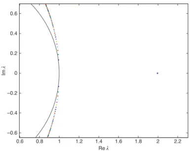
In Figure 3, for each value of r∈(1, 5), the distribution of eigenvalues is plotted for Π = Π_high. Note that one

eigenvalue is constant with respect to r, namely

Π

λ = = =

+ +

1 _{(1 ) 1 0.25305344n} 2.5 1.99512640877247.

The other eigenvalues come in complex conjugate pairs with Re λ= +1 1.

2 2r As r is close to 1, there exists a complex

conjugate pair close to the unit circle and as r diverges from 1, the real part decreases (see Figure 3). For this high level of regeneration rate Π_high, all the eigenvalues are outside the unit circle which results in a completely unstable system.

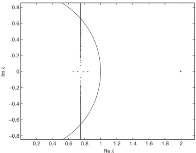
In Figure 4, for each value of r∈(1, 5), eigenvalues are plotted for Π = Π_low. The constant eigenvalue8 _{is left}

out for a better view. Now, the remaining eigenvalues totally stay inside the unit circle as r changes between 1.01 and 5. In this case, as r is close to 1, there exists a complex conjugate pair close to the unit circle boundary and as r increases, first the complex conjugate pair dissolve into two real roots and then the two real eigenvalues diverge from each other. However, for every level of r, these two (stable) eigenvalues along with the third (unsta-ble) one lead to a saddle path solution.

In the following example, we now take Π as the bifurcation parameter and numerically identify the Hopf bifurcation. 0.6 0.8 1 1.2 1.4 1.6 1.8 2 2.2 –0.6 –0.4 –0.2 0 0.2 0.4 0.6 Re λ Im λ

Figure 3: Eigenvalues distribution when Π = Πhigh as r∈(1, 5). The black curve is the boundary of the unit circle.

8 Also note that the value of this constant eigenvalue only depends on parameters α and β. Therefore the value when Π = Πlow is

Example 3 Recall the benchmark parametrization, i.e.

ρ=3, τ₁=1, τ₂=0.05, 0.33, α= and 0.98.β=

Further set r = 2. Π is a free parameter. Note that now the steady state value varies depending on the values of Π. In Figure 5, for each value of Π∈(2, 4), eigenvalues are plotted9 _{for r = 2. The constant eigenvalue has the same}

value (see footnote 8). For the first two iterations, real stable eigenvalues are observed. As Π further increases, eigenvalues become complex conjugates and then, crosses the unit circle. Note that, since r is constant, the real part of the complex eigenvalues is fixed. The figure clearly implicates that there exists a bifurcation value Π_Hopf such that a complex conjugate pair of eigenvalues with unit magnitude exists. Such a value designates the Hopf bifurcation. Numerically simulated, when

0.3 0.4 0.5 0.6 0.7 0.8 0.9 1 –0.3 –0.2 –0.1 0 0.1 0.2 0.3 Re λ Im λ

Figure 4: Eigenvalues distribution when Π = Πlow as r∈(1, 5). (The third constant eigenvalue omitted). The black curve is the

boundary of the unit circle.

0.2 0.4 0.6 0.8 1 1.2 1.4 1.6 1.8 2 –0.8 –0.6 –0.4 –0.2 0 0.2 0.4 0.6 0.8 Re λ Im λ

Figure 5: Eigenvalues distribution for Π∈(2, 4). The black curve is the boundary of the unit circle.

9  α β

β α + Π>

− 1.99513

2.15102282012,

Hopf

Π =

the eigenvalues are close to the unit circle with an error of 9.929834 × 10−13 _{in absolute value.}10

Koskela, Ollikainen, and Puhakka (2002, 2008) also examine the dynamic properties of an overlapping generation resource economy and ask whether the fundamentals can be a source of various types of observed cycles and complex dynamics. They demonstrate the existence of a flip bifurcation for the case of an ineffi-cient equilibrium.11 _{However, they assume a logistic resource growth function and require an implausibly low} values of the share of the resource in total output. Our setting allows us to obtain Hopf bifurcation without referring to logistic regeneration, shocks or constraints on parameter values and advocates the endogenous nonlinear interaction between population growth and resource availability.

4 Conclusion

In this paper, we have considered a nonlinear feedback mechanism between resource availability and popu-lation growth rate Through such a feedback mechanism we have shown that an overlapping generations resource economy can exhibit Hopf bifurcations. It is worthwhile to point out that the linear regeneration specification in our model provokes the question of how the stability of the system would change under a non-linear regeneration function. Allowing the renewable resource to regenerate non-linearly (e.g. logistic) could bring even more complex dynamics.

References

Accinelli, E., and J. G. Brida. 2005. “Re-Formulation of the Solow Economic Growth Model with the Richards Population Growth Law.” EconWPA at WUSTL 0508006.

Antoci, A., and M. Sodini. 2009. “Indeterminacy, Bifurcations and Chaos in an Overlapping Generations Model with Negative Environmental Externalities.” Chaos, Solitons and Fractals 42: 1439–1450.

Arrow, K., B. Bolin, R. Costanza, P. Dasgupta, C. Folke, C. S. Holling, B. Jansson, S. Levin, K. Maler, C. Perrings, and D. Pimentel. 1995. “Economic Growth, Carrying Capacity, and the Environment.” Science 268: 520–521.

Asea, Patrick K., and Paul J. Zak. 1999. “Time-to-Build and Cycles.” Journal of Economic Dynamics and Control 23: 1155–1175. Azariadis, Costas. 1993. Intertemporal Macroeconomics. Cambridge: Blackwell.

Benhabib, J., and R. E. A. Farmer. 1999. “Indeterminacy and Sunspots in Macroeconomics.” In Handbook of Macroeconomics, edited by J. Taylor and M. Woodford, 387–448. Vol. 1, North-Holland, Amsterdam.

Beverton, R. J. H., and S. J. Holt. 1957. “On the Dynamics of Exploited Fish Populations.” Fishery Investigations 19: 1–533. Brianzoni, S., C. Mammana, and E. Michetti. 2007. “Complex Dynamics in the Neoclassical Growth Model with Differential

Savings and Non-Constant Labor Force Growth.” Studies in Nonlinear Dynamics and Econometrics 11 (3): 1–17.

Capasso, Vincenzo, Ralf Engbers, Davide La Torre. 2012. “Population Dynamics in a Spatial Solow Model with a Convex-Concave Production Function.” In Mathematical and Statistical Methods for Actuarial Sciences and Finance, 61–68. Springer. Dasgupta, P., and G. Heal. 1979. Economic Theory and Exhaustible Resources. Cambridge: Cambridge University Press. de la Croix, D., and P. Michel. 2002. A Theory of Economic Growth: Dynamics and Policy in Overlapping Generations. Cambridge

University Press.

Faria, J. R. 2004. “Economic Growth with a Realistic Population Growth Rate.” Political Economy Working Paper 05/04. Farmer, Karl. 2000. “Intergenerational Natural – Capital Equality in an Overlapping – Generations Model with Logistic

Regeneration.” Journal of Economics 72 (2): 129–152.

10 The degree of error is within the acceptable limits considering the precision errors due to rounding of the numerical computing

environment.

11 As the notion of Pareto efficiency may not be well-defined in an endogenous population context, several alternative efficiency

concepts have been introduced (see e.g. Golosov, Jones, and Tertilt 2007; Michel and Wigniolle 2007). For the sake of comparison with Koskela, Ollikainen, and Puhakka (2008), we follow Willis (1987) and analyze the solution to the planning problem. Charac-terizing the conditions for the steady states under which they coincide with a competitive equilibrium, we obtain that the steady states are efficient if Π ≥ 1+n. Accordingly, the steady states around which we encounter Hopf bifurcation turn out to be efficient, in contrast with Koskela, Ollikainen, and Puhakka (2008).

Golosov, M., L. E. Jones, and M. Tertilt. 2007. “Efficiency with Endogenous Population Growth.” Econometrica 75 (4): 1039–1071. Grandmont, Jean-Michel., and G. Laroque. 1990. “Stability, Expectations and Predetermined Variables.” In Essays in Honor of

Edmond Malinvaud, vol. 1, Microeconomics, edited by P. Champsaur. Cambridge: MIT Press.

Grandmont, J.-M., P. Pintus, and R. de Vilder. 1998. “Capital-Labor Substitution and Competitive Nonlinear Endogenous Business Cycles.” Journal of Economic Theory 80: 14–59.

Kemp, M., and N. Van Long. 1979. “The Under-Exploitation of Natural Resources: A Model with Overlapping Generations.”

Economic Record 55: 214–221.

Kind, Christoph. 1999. “Remarks on the Economic Interpretation of Hopf Bifurcations.” Economic Letters 62: 147–154. Koskela, E., M. Ollikainen, and M. Puhakka. 2002. “Renewable Resources in an Overlapping Generations Economy without

Capital.” Journal of Environmental Economics and Management 43: 497–517.

Koskela, E., M. Ollikainen, and M. Puhakka. 2008. “Saddles and Bifurcations in an Overlapping Generations Economy with a Renewable Resource.” Finnish Economic Papers 21 (1): 3–21.

Michel, P., and B. Wigniolle. 2007. “On Efficient Child Making.” Economic Theory 31: 307–326.

Mourmouras, A. 1991. “Competitive Equilibria and Sustainable Growth in a Life–Cycle Model with Natural Resources.”

Scandinavian Journal of Economics 93 (4): 585–591.

Schtickzelle, M., and P. F. Verhulst. 1981. “La première découverte de la Function Logistique.” Population 3: 541–556. Seegmuller, T., and A. Verchère. 2007. “A Note on Indeterminacy in Overlapping Generations Economies with Environment and

Endogenous Labor Supply.” Macroeconomic Dynamics 11: 423–429. Smith, J. M. 1974. Models in Ecology. Cambridge: Cambridge University Press.

Valente, Simone. 2008. “Sustainable Development, Renewable Resources and Technological Progress.” Environmental and

Resource Economics 30: 115–125.

Wen, G., D. Xu, and X. Han. 2002. “On Creation of Hopf Bifurcations in Discrete-Time Nonlinear Systems.” Chaos 12 (2): 350–355. Willis, R. J. 1987. “Externalities and Population.” In Population Growth and Economic Development: Issues and Evidence, edited

by G. Johnson and R. D. Lee, 661–702. Madison, WI: University of Wisconsin Press.