AN OPTIMAL SOLUTION FOR THE MULTI-AGENT
RENDEZVOUS PROBLEM APPEARING IN
COOPERATIVE CONTROL
a thesis
submitted to the department of electrical and
electronics engineering
and the institute of engineering and sciences
of bilkent university
in partial fulfillment of the requirements
for the degree of
master of science
By
Fatih K¨olmek
September 2008
I certify that I have read this thesis and that in my opinion it is fully adequate, in scope and in quality, as a thesis for the degree of Master of Science.
Prof. Dr. Hitay ¨Ozbay (Supervisor)
I certify that I have read this thesis and that in my opinion it is fully adequate, in scope and in quality, as a thesis for the degree of Master of Science.
Prof. Dr. ¨Omer Morg¨ul
I certify that I have read this thesis and that in my opinion it is fully adequate, in scope and in quality, as a thesis for the degree of Master of Science.
Dr. Co¸sku Kasnako˘glu
Approved for the Institute of Engineering and Sciences:
Prof. Dr. Mehmet Baray
ABSTRACT
AN OPTIMAL SOLUTION FOR THE MULTI-AGENT
RENDEZVOUS PROBLEM APPEARING IN
COOPERATIVE CONTROL
Fatih K¨olmek
M.S. in Electrical and Electronics Engineering
Supervisor: Prof. Dr. Hitay ¨
Ozbay
September 2008
The multi-agent rendezvous problem appearing in cooperative control is consid-ered in this thesis. There are various approaches to this topic as the objectives and problem set-ups vary in real-life rendezvous problems. Some of the applica-tions can be given as the coordination of autonomous mobile robots or unmanned air vehicles (UAVs) for joint tasks, and motion planning for vehicle convoys. The problem is basically on providing a rendezvous for mobile agents at a specified or unspecified destination. What makes the topic interesting is maintaining a coordination between the mobile agents so that the agents reach the rendezvous point simultaneously. Early or late arrivals are not desired.
An energy optimal solution is obtained for the problem. Imperfect road conditions, obstacles, internal problems of the agents or similar disturbances are also tried to be handled. As these factors are included in the problem, it is assumed that the agents communicate between each other at specified time instants exchanging information about their expected arrival times in order to maintain a common rendezvous time among the team.
The solution is initially derived for rendezvous in one-dimensioned space. Then, the problem configuration is altered for two-dimensioned motions, and the target point is assumed to be moving in order to extend the solution to possible practical applications. The effect of increasing disturbance on the control input and time delays in the communication are also discussed.
Keywords: Multi-Agent Rendezvous Problem, Optimal Control, Cooperative
¨
OZET
˙IS¸B˙IRL˙IKL˙I KONTROLDE G ¨OR¨ULEN C¸OK ARAC¸LI
BULUS¸MA PROBLEM˙I ˙IC
¸ ˙IN OPT˙IMAL B˙IR C
¸ ¨
OZ ¨
UM
Fatih K¨olmek
Elektrik ve Elektronik M¨uhendisli¯gi B¨ol¨um¨u Y¨uksek Lisans
Tez Y¨oneticisi: Prof. Dr. Hitay ¨
Ozbay
Eyl¨ul 2008
Bu tezde, i¸sbirlikli kontrolde g¨or¨ulen ¸cok ara¸clı bulu¸sma problemi ele alınmaktadır. Bu konuya yapılan yakla¸sımlar, ger¸cek hayattaki bulu¸sma prob-lemlerinin ama¸clarının ve problem d¨uzeneklerinin birbirlerinden farklı olması nedeniyle ¸ce¸sitlilik g¨osterir. Problemin bazı uygulamalarına ¨ornek olarak, hareketli ¨ozerk robotların veya insansız hava ara¸clarının (˙IHA) birle¸sik g¨orevler i¸cin koordine edilmesi ve ara¸c konvoyları i¸cin hareket planlaması verilebilir. Problem temel olarak, hareketli ara¸cların belirli veya belirsiz bir varı¸s nok-tasında bulu¸smalarının sa˘glanmasına dayalıdır. Konuyu ilgin¸c kılan ¸sey, erken veya ge¸c varı¸slar istenen durumlar olmadı˘gından, bulu¸smanın aynı anda ger¸cekle¸smesini sa˘glayacak ¸sekilde hareketli olan ara¸clar arasında bir koordinasy-onun sa˘glanmasıdır.
Problem i¸cin enerji a¸cısından optimal bir ¸c¨oz¨um elde edilirken, m¨ukemmel olmayan yol durumlarının, engellerin, ara¸cların i¸csel problemlerinin veya benzer bozucu etkilerin de ele alınmasına ¸calı¸sılmaktadır. Bu etkenler probleme dahil edildi˘ginden, ara¸cların takım i¸cerisinde ortak bir bulu¸sma zamanı belirleyebilmek i¸cin, birbirleri arasında muhtemel varı¸s zamanları hakkında bilgi alı¸s veri¸sinde bulunmak ¨uzere haberle¸stikleri kabul edilmektedir.
C¸ ¨oz¨um ba¸slangı¸cta bir boyutlu uzaydaki bulu¸sma i¸cin geli¸stirilmektedir. Son-rasında ise, problemin konfig¨urasyonu iki boyutlu hareketler i¸cin de˘gi¸stirilmekte ve ¸c¨oz¨um¨un muhtemel pratik uygulamaları kapsayacak ¸sekilde geni¸sletilebilmesi i¸sin hedef noktasının hareket etti˘gi varsayılmaktadır. Ayrıca, kontrol girdisi ¨uzerindeki bozucu etkilerin ve haberle¸smedeki zaman gecikmelerinin artması du-rumları da tartı¸sılmaktadır.
Anahtar Kelimeler: C¸ ok Ara¸clı Bulu¸sma Problemi, Optimal Kontrol, ˙I¸sbirlikli Kontrol, Minimum Enerji Kontrol¨u, De˘gi¸simler Hesabı.
ACKNOWLEDGMENTS
I would like to gratefully thank my supervisor Prof. Dr. Hitay ¨Ozbay for his guidance, support and encouragement throughout my graduate study.
I would like to thank the members of my thesis committee Prof. Dr. ¨Omer Morg¨ul and Dr. Co¸sku Kasnako˘glu for reading and commenting on this thesis.
I would like to thank my colleagues and our group head Rıza G¨ung¨or at EPDK for their support and encouragement.
I would like to thank my family for always being by my side whenever I needed.
Finally, I would like to express my special thanks to my wife for her endless support, encouragement, patience and understanding while writing this thesis.
Contents
1 INTRODUCTION 1
1.1 Cooperative Control . . . 2
1.2 Optimal Control . . . 3
1.3 Rendezvous Problem . . . 4
1.4 Thesis Contribution and Organization . . . 8
2 PROBLEM STATEMENT AND PRELIMINARIES FROM OPTIMAL CONTROL THEORY 9 2.1 Description of the Problem . . . 9
2.2 Preliminaries from Optimal Control Theory . . . 12
2.2.1 Calculus of Variations . . . 12
2.2.2 Minimum Energy Control . . . 18
2.3 Adaptation of the Solution to the Multi-Agent Rendezvous Problem 22 3 APPLICATION TO RENDEZVOUS PROBLEMS 25 3.1 Multi-Agent Rendezvous Problem in 1-D . . . 25
3.1.1 Three-Vehicle Rendezvous Problem . . . 26
3.1.2 Three-Vehicle Rendezvous Problem in the Presence of Communication Problems . . . 29
3.2 Multi-Agent Rendezvous Problem in 2-D . . . 46
3.2.1 2-D Rendezvous Problem with Fixed Target . . . 46
3.2.2 2-D Rendezvous Problem with Moving Target . . . 49
3.2.3 2-D Rendezvous Problem with Moving Target in the Pres-ence of Communication Problems . . . 52
3.3 Effects of Increasing Disturbance and Time Delay on the Solution 57 3.3.1 Increasing Disturbance . . . 58
3.3.2 Increasing Time Delay . . . 62
4 CONCLUSIONS 66
APPENDIX 68
A Matlab code for the solution of rendezvous in 1-D 68
List of Figures
2.1 Rendezvous problem for N vehicles . . . 10
2.2 Position, velocity and control input for t0
i = 0, tfi = 10 . . . 16
2.3 Position,velocity and control input for t0
i = 0, tfi = 5 . . . 16
2.4 Position, velocity and control input for t0
i = 0, tfi = 3 . . . 17
2.5 Position, velocity and control input for t0
i = 0, tfi = 5 in minimum
energy control . . . 21
2.6 Position, velocity and control input for t0
i = 0, tfi = 10 in minimum
energy control . . . 21
2.7 Position & control inputs vs. time for t0
i = 0, tfi = 10 in minimum
energy control . . . 24 2.8 Change in tf at communication instants for t0i = 0, tfi = 10 in
minimum energy control . . . 24
3.1 Positions vs. time for rendezvous in 1-D without communication problems . . . 27
3.2 Control inputs vs. time for rendezvous in 1-D without communi-cation problems . . . 28
3.3 Change in tf at communication instants for rendezvous in 1-D
without communication problems . . . 28
3.4 Positions vs. time for rendezvous in 1-D with one-way time delays in communication . . . 32
3.5 Control inputs vs. time for rendezvous in 1-D with one-way time delays in communication . . . 33 3.6 Velocities vs. time for rendezvous in 1-D with one-way time delays
in communication . . . 34 3.7 Accelerations vs. time for rendezvous in 1-D with one-way time
delays in communication . . . 34
3.8 Change in tfis at communication instants for rendezvous in 1-D with one-way time delays in communication . . . 35
3.9 Positions vs. time for rendezvous in 1-D including communication problems . . . 39 3.10 Control inputs vs. time for rendezvous in 1-D including
commu-nication problems . . . 39
3.11 Velocities vs. time for rendezvous in 1-D including communication problems . . . 40
3.12 Accelerations vs. time for rendezvous in 1-D including communi-cation problems . . . 40
3.13 Change in tfis at communication instants for rendezvous in 1-D including communication problems . . . 41 3.14 Positions vs. time for rendezvous in 1-D including communication
3.15 Control inputs vs. time for rendezvous in 1-D including commu-nication problems . . . 44
3.16 Velocities vs. time for rendezvous in 1-D including communication problems . . . 44
3.17 Accelerations vs. time for rendezvous in 1-D including communi-cation problems . . . 45 3.18 Change in tfis at communication instants for rendezvous in 1-D
including communication problems . . . 45 3.19 Position trajectories for rendezvous in 2-D with fixed target . . . 48
3.20 Velocities vs. time for rendezvous in 2-D with fixed target . . . . 48
3.21 Position trajectories for rendezvous in 2-D with moving target . . 51 3.22 Velocities vs. time for rendezvous in 2-D with moving target . . . 51
3.23 Position trajectories for rendezvous in 2-D with moving target . . 53 3.24 Velocities vs. time for rendezvous in 2-D with moving target . . . 54
3.25 Change in tfis at communication instants for rendezvous in 2-D with moving target . . . 54 3.26 Position trajectories for rendezvous in 2-D with moving target
including communication problems . . . 56
3.27 Velocities vs. time for rendezvous in 2-D with moving target in-cluding communication problems . . . 56
3.28 Change in tfis at communication instants for rendezvous in 2-D with moving target including communication problems . . . 57
3.29 Position trajectories for increasing disturbances . . . 59
3.30 Magnitudes of the control inputs vs. time for increasing disturbances 60
3.31 Final times vs. time for increasing disturbances . . . 61 3.32 Position trajectories for increasing time delay in the communication 63
3.33 Magnitudes of the control inputs vs. time for increasing time delay in the communication . . . 64
List of Tables
3.1 Calculated Final Time tf w.r.t. the communication instant . . . . 30
3.2 Final Times in the absence of time delays hiks . . . 30
3.3 Communication delays hik in sec. for corresponding instants k . . 31
3.4 Final Times in the presence of time delays hiks . . . 31
3.5 Calculated Final Times tfi(k) w.r.t. the communication instant . . 36 3.6 Final Times in the absence of time delays hij(k)s . . . . 37
3.7 Final Times in the presence of time delays hij(k)s . . . . 38
3.8 Calculated Final Times tfi(k) w.r.t. the communication instant . . 41
3.9 Final Times in the absence of time delays hij(k)s . . . . 42
Chapter 1
INTRODUCTION
In this thesis, we investigate optimal solutions for a rendezvous problem appear-ing in cooperative control. The problem in question is gettappear-ing N > 1 vehicles in a task force to reach a specified point at the same time instant. It is assumed that these vehicles communicate with each other exchanging information about their expected final time to reach the rendezvous point in order to avoid early or late arrivals, and this communication occurs at discrete time instants.
The interesting part of the problem is that the final times of the vehicles may change during the mission due to unforeseen events, like obstacles on the road or internal problems of the vehicles, and there might be time delays in the communication between the vehicles. Therefore, a satisfactory solution for the stated rendezvous problem should take these conditions into account and provide reliable results in order to be applicable.
Before attacking the problem, let us give some information about the concepts related with the subject and present a brief information about the similar studies in the literature.
1.1
Cooperative Control
Research on control of multi-vehicle systems performing cooperative tasks gained importance in the late 1980s [1] when several researchers began investigations in multiple mobile robot systems [2]. Since then, the interest in this topic has increased significantly thanks to the development of inexpensive and reliable wireless communications systems and the application fields in military operations [1].
The most popular problems of cooperative control of mobile robots involve groups or teams of autonomous vehicles cooperating to complete a mission [3]. Basically, the success of the mission can only be attained when none of the vehicles or groups that are performing separate tasks fail, i.e. each individual performing the corresponding task must succeed. The interesting part of the problem is that the vehicles or the groups have to perform coordinated actions [3] in order to complete their individual tasks.
At this point, it is helpful to give a concise explanation about what is meant by
cooperative control before going into more detail in the subject. A comprehensive
study about the recent researches on the topic can be found in [1].
Consider a group of vehicles aiming to complete a task and the corresponding overall performance function below.
J =
Z T
0
L(x, α, u)dt + V (x(T ), α(T )) (1.1)
where x is the states, α is the roles, T is the final time that the task should be completed, L is the incremental cost of the task and V represents the terminal cost of the task. Notice that (1.1) is a typical cost function.
J = N X i=0 µZ T 0 Li(xi(t), αi(t), ui(t))dt + Vi(xi(T ), αi(T )) ¶ (1.2) where
i : the index corresponding to vehicle i xi(t) : the state of vehicle i at time t
αi(t) : the role of vehicle i at time t that is
subject to change during the task
ui(t) : the input controlling the state of vehicle i at time t
xi(T ) : the final value of the state of vehicle i
αi(T ) : the final value of the role of vehicle i
otherwise, the task is called coupled or namely cooperative which means that the task performance depends on the joint locations, roles and inputs of the vehicles [1].
Then, cooperative control can simply be defined as determining the control law ( i.e. the control input ui(t)) that solves the coupled performance function
which is the dual of (1.2) corresponding to a cooperative task defined above.
1.2
Optimal Control
Optimal control can basically be described as the problem of determining a con-trol law for a given system while satisfying the specified optimality conditions. A precise mathematical description can be given as finding an admissible control
u∗(t) which forces the following system with x(t) as the state, u(t) as the control
˙x(t) = f (x(t), u(t), t) (1.3)
to follow an admissible trajectory x∗(t) that minimizes or maximizes the
perfor-mance measure in the form
J = h(x(tf), tf) +
Z tf
t0
g(x(t), u(t), t)dt (1.4)
with u∗(t) being the optimal control input and x∗(t) being the optimal trajectory
[4]. Here, f, g, h are specified functions that satisfy certain assumptions, see e.g. [4].
In this study, the solutions for the multi-agent rendezvous problem are to be optimal with constraints like fixed initial and final states, and the cost to be minimized is the control energy. Therefore, we will form a performance measure as in (1.4) that involves the constraints to be considered, and solve for the optimal input resulting in a successful rendezvous.
1.3
Rendezvous Problem
The multi-agent rendezvous problem in this thesis is an optimal control problem appearing in cooperative control. The idea is having a number of mobile agents arrive at a meeting point, namely the rendezvous point, at the same time. The crucial point is assuring that the agents perform cooperative actions by arranging themselves according to the information gathered from the other agents in the team [5].
Actually, the title “rendezvous problem” is a broad one, and it is a general name for various problems in cooperative control some of which are;
The problem of two aircrafts aiming to meet at a non-specified point at a predefined final time [6],
The problem of trajectory planning for the vehicles in a team aiming to reach the neighborhood of a point not before the other vehicles in the team [7],
The problem of path planning for a robot aiming to reach a target [8, 9], The coordination of unmanned aerospace vehicles (UAVs) to reach a target
point [10],
The problem of enabling mobile users in a location, tracking and rendezvous with a variety of mobile entities [11],
The problem of conflict management in a multi-user computer network [12], The problem of motion planning for vehicle convoys [13],
The problem of multi-agent rendezvous [14–17],
Probably, the most popular one of the problems above is the multi-agent rendezvous problem which is the subject discussed in this thesis. The popularity is basically due to variety of applications in military operations ranging from cooperative attack in land operations to cooperative control of unmanned air vehicles (UAVs) for rendezvous in air operations. In the literature there are many versions of this problem involving constraints such as rendezvous with fixed final time, time optimal rendezvous with unspecified final states, and energy efficient rendezvous. Next, some of the solutions to similar rendezvous problems are presented.
In one of the studies related with the multi-agent rendezvous, the problem of determining a meeting point while minimum energy consumption is taken into account is discussed [18]. In that paper, a multi-robot team, which consists
of autonomous mobile robots trying to meet at a single point for a mission, is considered, and two solutions about the minimum energy consumption during the travels towards the rendezvous point are proposed. The interesting part of the problem is that the cost of travel for each robot is different and the goal is to find an energy efficient solution considering the robots in the team as a whole. Although the proposed solutions are successful in finding a rendezvous point, the proposed algorithms do not consider a timing constraint. In addition, as indicated in the paper, the solutions assume a reliable communication between the robots, and communication delays or loss of information about the current positions of the robots are not handled.
A similar problem on multi-agent rendezvous is considered in [15,16]. In that setting, there are N > 1 vehicles aiming to meet at an unspecified point which is regarded as rendezvous by sensing the current positions of the neighboring mobile agents that are within their sensing region. The presented solution is basically determining decentralized control algorithms for the agents. In other words, the solution just guarantees the rendezvous for the agents but does not include the constraints on the control energy, the final states (velocity and acceleration) of the agents, and imperfect communication.
Another related study about the multi-agent rendezvous problem is on the stability of mobile robot rendezvous [8]. In this study, a mobile robot aiming to reach a target point is considered, and an optimal control is derived. In that problem, the destination point and the final time is specified for an autonomous robot, and the robot aims to arrive the rendezvous point on time while evaluat-ing its current states with respect to the rendezvous point and arrangevaluat-ing itself accordingly via applying a step control acceleration. Both 1-D and 2-D solutions are provided assuming that the states are known and there is no noise or distur-bance in the system. Besides, the solutions are derived for a single autonomous robot and thus exclude a cooperative control scheme and communication with
a central point or any other agent. Moreover, the resulting control inputs have large magnitudes and there is a possibility of instability as the robots gets closer to the rendezvous point, for that reason a limit is placed on the applied control input.
A very similar work is presented in [19] in which a multi-robot rendezvous problem is discussed. The goal of the problem is to determine control laws for
N robots moving in the horizontal plane in order to reach a moving robot at
the same time. The motion of the moving robot, namely the reference-robot is not a priori known by other robots aiming to catch it. It is assumed that all robots move faster than the reference robot, the motion of the reference robot is continuous and there is a reliable communication between the leader robot and the others, and a sensory system in order to determine the position of the reference robot. In that paper two approaches for the solution are presented.
First one is the leader-follower approach in which the leader of the team tracks the position of the reference robot and the team members try to follow the leader. Since the leader perfectly tracks the reference-robot and the others catch the leader eventually, all the robots catch the reference robot consequently. In that approach, it is also assumed that the followers move faster than their leader.
The second one is the reference-robot approach in which all the robots sense the position of the reference robot continuously and try to catch it. Since all the robots move faster than the reference robots, all the robots in the team catches the reference-robot successfully.
The solutions are obtained via relative kinematic equations and they are suc-cessful as all the robots catch the reference-robot at the same time. However,
the solutions include neither time nor energy optimality constraints, and it is as-sumed that there is no communication deficiency like lost or delayed information signals between the robots.
1.4
Thesis Contribution and Organization
In the following chapters, the multi-agent rendezvous problem in question is described, the mathematical solution is derived and the application results are presented. The major advantage of the solutions given here is being optimal in terms of the control energy used by the mobile agents while providing a suc-cessful rendezvous with pre-specified initial and final states. Moreover, delayed communication for simultaneous cooperative rendezvous is handled.
Remaining parts of the thesis are organized as follows. In Chapter 2, the configuration of the multi-agent rendezvous problem is described and the basics of the mathematical solution are introduced together with some simple illustrative examples. The application of the solution to the problem is given in Chapter 3. The solutions for rendezvous in 1-D in the presence/absence of communication problems modeling delayed or lost information about the estimated times of arrivals are presented. The solution is extended to 2-D and the case of moving target point is addressed for practical applications. The effect of increasing disturbance on the control input and time delays in the communication are also discussed. Chapter 4 includes the conclusions and some notes about possible complementary studies to be made.
Chapter 2
PROBLEM STATEMENT AND
PRELIMINARIES FROM
OPTIMAL CONTROL
THEORY
In this chapter, the description of the multi-agent rendezvous problem is given. Basic concepts and tools from optimal control theory are described in order to establish a background for the problem solution.
2.1
Description of the Problem
As stated in the introduction briefly, we will discuss a rendezvous problem ap-pearing in cooperative control. Remember that there are N > 1 vehicles in a task force and their goal is to reach a target point(rendezvous point) at the same time instant spending as low energy as possible. It is assumed that they com-municate with each other at specified time instants during their mission in order
to arrange their states so that they all arrive the target point at the same time instant, neither before nor after.
Consider the rendezvous problem for N vehicles illustrated in Figure 2.1. The vehicles aim to reach the target point ptat the same time instant. Basically,
one can assign a final time tf for the mission and inform the vehicles to be
at the target point at time tf and the vehicles arrange their acceleration or
velocity accordingly. However, if one of the vehicles fails to be at pt at time
tf due to an internal problem or bad road conditions, the mission may not be
completed successfully. In order to overcome that problem, it is better to utilize an information exchange between the vehicles about their position, velocity and acceleration or just the estimated time of arrival at discrete time instants. Thus, at each information exchange instant the vehicles can use the information that they received from the other vehicles in the team as a feedback to arrange their states and try to catch the fastest or the slowest of the team in order to arrive the rendez-vous point pt at the same instant.
Consider the following dynamical model for the vehicles
˙
xi(t) = f (xi(t), ui(t), wi(t)) (2.1)
where f is a known function of the state xi, input ui and the disturbance wi. The
state xi consists of the position, velocity and the acceleration of the ith vehicle
in space. In order to simplify the problem we may consider the following linear case assuming that wi(t) = 0:
˙ xi(t) = Aixi(t) + Biui(t) (2.2) where Ai = 0 1 0 0 0 1 0 0 0 , Bi = 0 0 1
. The target point is assumed be fixed at the origin. In order to determine the solution guaranteeing the success of the mission, the following quadratic cost function should be solved for the minimizing optimal control input ui(t):
Ji(t) = Z tf i t (kxi(τ )k2Qi+ kui(τ )k 2 Ri)dτ + kxi(t f i)kQfi (2.3)
where Qi, Riand Qfi are the weighting matrices of appropriate dimensions. What
makes the problem interesting is that in the equation above, the final time tfi is time varying, and is updated at discrete time instants tk depending on the
feedback received from the other vehicles. There are two choices:
tfi(t) = min{t1f(t), t2f(t), t3f(t), . . . , tN f(t)} (2.4)
or
tfi(t) = max{t1f(t), t2f(t), t3f(t), . . . , tN f(t)} (2.5)
where tjf(t) is the expected time of arrival for the jth vehicle at time t, and is a
We can denote tjf(t) as tjf(t) = p(xjp(t), vjp(t), ajp(t), uj(t)), where xjp(t),
xjv(t), xja(t) and uj(t) are the position, velocity, acceleration and control input
of the jth vehicle at time t, respectively. Here, p is a function to determine the final time of a vehicle by assuming that current optimal control input u∗
i(t) will
not be subject to any change during the rest of the travel. Note that, tfi(t) is generated from a data set of N received by the ith vehicle up to time t. In order to have a more realistic problem, it is convenient to assume that there are time delays in the communications between each vehicle, i.e.:
tfi(t) = min{t1f(t − h1i(t)), tf2(t − h2i(t)), tf3(t − h3i(t)), . . . , tfN(t − hN i(t))} (2.6)
or
tfi(t) = max{tf1(t − h1i(t)), tf2(t − h2i(t)), tf3(t − h3i(t)), . . . , tfN(t − hN i(t))} (2.7)
where hji(t) represents the time delay in the one way communication from vehicle
j to vehicle i at time instant t.
2.2
Preliminaries from Optimal Control Theory
In this section the solution of the rendezvous problem described in Section 2.1 is presented using basic principles from optimal control theory. For the time being, suppose that the information exchange between the vehicles is perfect and not effected by the delay. Then, we can proceed with the solution of the quadratic cost function minimization problem.
2.2.1
Calculus of Variations
Suppose that the state xi(t) is composed of position and velocity of the ith vehicle
only, i.e. Ai = 0 1 0 0 , Bi = 0 1 (2.8)
where Qi = I2×2, Ri = I2×1, Qfi = I2×2 and the initial and the final conditions
xi0 and xif are known.
Optimal solution of the quadratic cost function minimization problem defined by (2.3) can be obtained by “Calculus of Variations” which is a well-known method for solving optimal control problems. As explained in [4], the necessary conditions for optimality in order to solve the problem are:
˙x∗ i = ∂H ∂p( ˙x ∗ i(t), ˙u∗i(t), ˙p∗i(t), t) ˙p∗i = ∂H ∂x( ˙x ∗ i(t), ˙u∗i(t), ˙p∗i(t), t) 0 = ∂H ∂ui ( ˙x∗ i(t), ˙u∗i(t), ˙p∗i(t), t) (2.9)
for all t ∈ [t0, tf], where H is the Hamiltonian defined as
H(x(t), u(t), p(t), t) , g(x(t), u(t), t) + pT(t) [f (x(t), u(t), t)] (2.10) and · ∂h ∂x(x ∗(t f) − p∗(tf)) ¸T ∂xf + · H(x∗(t f), p∗(tf), tf) + ∂h ∂t(x ∗(t f), tf) ¸ ∂tf = 0 (2.11)
for the system and the cost function below
˙ xi(t) = f (xi(t), ui(t), t) (2.12) J(u) = h(x(tf), tf) + Z tf t0 g(x(t), u(t), t)dt (2.13)
At this point, it is not difficult to construct an analogy between (2.3) and (2.13) as follows
h(x(tf), t) = kxi(Tif(t))kQfi
g(x(tf), t) = kxi(τ )k2Qik + kui(τ )k
2
In (2.11), p∗(t) represents the Lagrange multipliers p∗
1(t), p∗1(t), . . . , p∗n(t)
which are selected as follows.
˙p∗(t) = − · ∂f ∂x(x ∗(t), u∗(t), t) ¸T p∗(t) − · ∂g ∂x(x ∗(t), u∗(t), t) ¸ (2.15)
Note that, p(t) is also called costate and the equation above is called costate
equations. By solving the equations (2.9) and (2.11), the costates, the optimal
control input and the output trajectory can be obtained easily.
If we apply (2.9)-(2.15) to our simplified problem, we can have the following formulation [4].
The Hamiltonian for the problem is
H(x(t), ui(t), pi(t), t) = 1 2x TQ ixi(t) + 1 2u TR iui(t) + pTA ix(t) + pTi (t)Biui(t) (2.16)
Then, the necessary conditions for the solution in order to exist are ˙x∗ i = Aix∗i(t) + Biu∗i(t) (2.17) ˙p∗ i = ∂H ∂xi = −Qix∗i(t) − ATi p∗i(t) (2.18) 0 = ∂H ∂u = Riu ∗ i(t) + BiTp∗i(t) (2.19)
Notice that the optimal control input ui(t) can be obtained from (2.19) as
u∗
i(t) = −R−1i BiTp∗i(t) (2.20)
Substituting (2.20) into (2.17) yields
x∗
Combining (2.21) and (2.18) we have 2n linear differential equations which are formulated below.
˙x∗i(t) ˙p∗ i(t) = Ai −Qi −BiRi−1BiT −AT i x∗i(t) p∗ i(t) ˙x∗i(t) ˙p∗ i(t) = Φ x∗i(t) p∗ i(t) (2.22)
where Φ is the transition matrix. In order to solve (2.22) we need 2n boundary conditions, and we already have them as xi(t0) = x0i and xi(tf) = xfi. The rest
of the solution in order to determine the Lagrange multipliers p∗
i(t), the control
input u∗
i(t) and the states x∗i(t) is trivial and can be obtained easily after solving
(2.22) for x∗
i(t) and p∗i(t) by following the steps explained in [20]. Remember
that the solution of a set of the 2n linear differential equations will be in the form below x∗i(t) p∗ i(t) = c1eλ1tv1 + c2eλntv2t + . . . + cneλntvn (2.23)
where cis are the coefficients, and λis and vis are the eigenvalues and the
eigen-vectors of Φ, respectively. Now, let us look at some sample results obtained by the explained method.
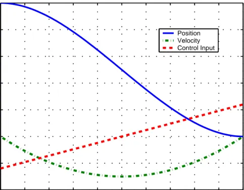
The solutions for x0
i = 5 0 , xf i = 0 0 , t0 i = 0, tfi = 10 and tfi = 5 are
depicted in Figures 2.2 and 2.3, respectively. In that figures, it can be observed that the optimal control input u∗
i(t) for the cost function in (2.3) brings the
vehicle to the rendezvous point at nearly t = 5 whereas the rendezvous time was specified as tfi = 10 initially, and no change were made during the travel.
0 1 2 3 4 5 6 7 8 9 10 −6 −4 −2 0 2 4 6 time output Position Velocity Control Input
Figure 2.2: Position, velocity and control input for t0
i = 0, tfi = 10 0 0.5 1 1.5 2 2.5 3 3.5 4 4.5 5 −6 −4 −2 0 2 4 6 time output Position Velocity Control Input
Figure 2.3: Position,velocity and control input for t0
This result is basically due to the configuration of the cost function, because the optimal control input is determined by taking the constraints for the control energy and the difference between the current and final states to be reached into account directly. In other words, the control input tries to bring the vehicle to the rendezvous point just on time using minimum control energy but it also forces the states to converge to zero as soon as possible. Thus, we observe that the vehicle reaches the target point much before the specified time.
Moreover, as seen below for x0
i = 5 0 , xf i = 0 0 , t0 i = 0 and tfi = 3,
if the specified final time is close to the departure time (i.e. the travel time is short) the control input grows too much, and such a case is not acceptable due to the practical limits of the controller. Therefore, a realizable solution is needed and the next section addresses this problem.
0 0.5 1 1.5 2 2.5 3 −6 −4 −2 0 2 4 6 time output Position Velocity Control Input
Figure 2.4: Position, velocity and control input for t0
2.2.2
Minimum Energy Control
Regarding the results obtained by solving the cost function in (2.3), it can be concluded that the obtained control input does not solve the problem appropri-ately due to the constraints included in cost function. Having known the reasons, it might be possible to improve the solution.
For instance, the term kxi(tfi)kQfi has no relevance with the minimization of
the control input to be used since xfi = 0, and it can be excluded. Moreover, including the term kxi(t)k2Qi in the cost function to be minimized results in a
struggle for an early arrival to the rendezvous point (i.e. tfi) and consequently the usage of more energy in the control input. So, we may also exclude that term in the cost function and have the new cost function to be minimized as follows.
Ji(t) = 1 2 Z tf i t0 i (kui(t)k2Ri)dt (2.24)
Now, the question is “How can we guarantee that the vehicle reaches the rendezvous point having excluded the states in the cost function?” and the answer is simple. The control input and the states are related by the system equation in (2.2) with Ai and Bi as in (2.8). Therefore, although the term
related with the states is not involved in (2.24), the optimal solution of (2.24) gives not only the minimum energy signal (i.e. the control input ui(t)) but also
the desired state trajectory since the solution is based on the time constraint of
t0
i and tfi, and the boundary conditions of xi(t0i) = x0i and xi(tfi) = xfi. Thus,
we will solve another cost function minimization problem known as “Minimum Energy Control Problem”.
Solution of the minimum energy control problem is based on “Calculus of Variations Method” and basically aims to minimize the control energy in the
cost function of (2.24). Thus, it is expected that the optimal control input will not grow much enabling the vehicle to reach the target point just on time.
As minimum energy control control is a very well known issue, the lengthy derivation of the optimal control input and the minimum cost can be found in many books like [21], [6] and [4]. Here, the derivation is skipped and only the solution is presented, however the reader is referred to [21] for a detailed derivation with a comprehensive explanation on the topic.
Notice that the controllability Gramian for the system in (2.2) with Ai and
Bi as in (2.8) Wc(t0i, tfi) = Z tf i t0 i eAi(t0i−τ )B iBiTeA T i(t0i−τ )dτ (2.25)
is nonsingular for any tfi > t0
i since (Ai, Bi) is a controllable pair. Then, the
minimum energy control signal ui(t) can be obtained as
u∗ i(t) = −BiTeA T i(t0i−t)W−1 c (t0i, tfi)(x0i − eAi(t 0 i−t f i)xf i) (2.26)
Alternatively, the minimum energy control signal can be written in terms of the reachability Gramian Wr as
Wr(t0i, tfi) = Z tf i t0 i eAi(tfi−τ )B iBiTeA T i(tfi−τ )dτ (2.27) and u∗i(t) = −BiTeATi(t f i−t)W−1 r (t0i, tfi)(xfi − eAi(t f i−t0i)x0 i) (2.28)
Then, the minimum energy value J∗ i can be determined as J∗ i = 1 2 Z tf i t0 i ku∗ i(t)k2dt = 1 2(x 0 i − eAi(t 0 i−t f i)xf i)TWc−1(t0i, tfi)(x0i − eAi(t 0 i−t f i)xf i) (2.29)
For the controllable pair (Ai, Bi) in (2.8) and the boundary conditions x0i =
5 0 and xf i = 0 0 with t0
i = 0 and tfi = 5, Wc and u∗i(t) are calculated as
Wc(t0i, tfi) = 13(t f i − t0i)3 − 12(t f i − t0i)2 −1 2(t f i − t0i)2 (tfi − t0i) = 1253 − 252 −25 2 53 u∗ i(t) = 12 25t − 6 5 (2.30)
Then, the trajectory of xi(t) can easily be calculated as
x∗ i(t) = eAi(t−t 0 i)+ 252t3− 35t2 6 25t2− 65t = 1 5 0 1 5 0 + 252 t3− 35t2 6 25t2 −65t = 5 0 + 252t3−35t2 6 25t2− 65t (2.31)
which is plotted in Figure 2.5.
The optimal solution for tfi = 10 is also plotted in Figure 2.6. Comparing Figures 2.2 and 2.3 with Figures 2.5 and 2.6, one can observe that the minimum energy control solution provides the desired rendezvous results unlike the former one.
0 0.5 1 1.5 2 2.5 3 3.5 4 4.5 5 −2 −1 0 1 2 3 4 5 time output Position Velocity Control Input
Figure 2.5: Position, velocity and control input for t0
i = 0, tfi = 5 in minimum energy control 0 1 2 3 4 5 6 7 8 9 10 −1 0 1 2 3 4 5 time output Position Velocity Control Input
Figure 2.6: Position, velocity and control input for t0
i = 0, tfi = 10 in minimum
2.3
Adaptation of the Solution to the
Multi-Agent Rendezvous Problem
Up to this point, the solution was for the optimal control of one vehicle, and now the question is: “How can we include other vehicles in the team and the communication between them in order to update the rendezvous instant and get all of the vehicles to be at the target point just at the rendezvous time?” The answer is discussed next.
Remember that the optimal solution of the rendezvous problem is u∗
i(t) which
minimizes the cost function in (2.24) with respect to the boundary conditions (i.e. the initial and the final states). Now, suppose that the vehicles communicate at each discrete time instant tk and the rendezvous time is updated or remain
unchanged with respect to the received information. Then, we can solve for u∗ i(t)
by accepting x0
i as the value of the states at the communication instant and xfi
as the value of the states at the rendezvous instant.
Knowing the exact values of the states at the communication instant and the required distance to be traveled, it is not so difficult to solve for tfnew
i which is
the new rendezvous time for vehicle i. In order to determine tfnew
i at time tk, it
is assumed that the current optimal control input u∗
i(t) will not change during
the rest of the travel. That means the trajectory of the ith vehicle’s position will remain the same during the rest of the travel. As seen in (2.31), the trajectory of the position of vehicle i (i.e. xip(t)) is a third order polynomial of t. Similarly,
xip(t) will be a fifth order polynomial of t when we include the acceleration in
our model. So, we can express xip(t) as
Then, we can express the distance to be traveled by vehicle i as
xfip− x0ip = ∆xip
= an(tfinew)n+ an−1(tifnew)n−1+ . . . + a1tfinew −
¡
an(tk)n+ an−1(tk)n−1+ . . . + a1(tk)
¢
(2.33)
in order to determine tfnew
i . Here, x0ip and xfip are the positions of vehicle i at
the communication instant tk and the rendezvous time, respectively. We can
determine the coefficients an, an−1, . . . , a1 at the communication instant by using
the previous values of xip. Then, we can solve (2.33) for tfinew and determine the
new rendezvous time for vehicle i.
By repeating this procedure at the communication instants, each vehicle can determine its own expected arrival time, and the rendezvous time can be found accordingly by (2.4) or (2.5). Notice that choosing (2.4) instead of (2.5) is better for the success of the mission since (2.5) means that the vehicles in the team follows the slowest vehicle and this may result in increasing tfi values tending to infinity.
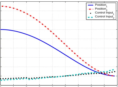
A sample solution for the 2-vehicle rendezvous problem below is presented next: ˙xi = Aixi(t) + B1iui(t) + B2iwi(t), t0 = 0, tf = 10, x1(t0) = 10 0 , x1(tf) = 0 0 , x2(t0) = 15 0 , x2(tf) = 0 0 (2.34) where Ai = 0 1 0 0 , B1i = 0 1
, B2iwi(t) is an appropriate random
sig-nal accounting for imperfect road conditions or any other reason disturbing the current position of the vehicle i, and vehicles communicate every 2 seconds.
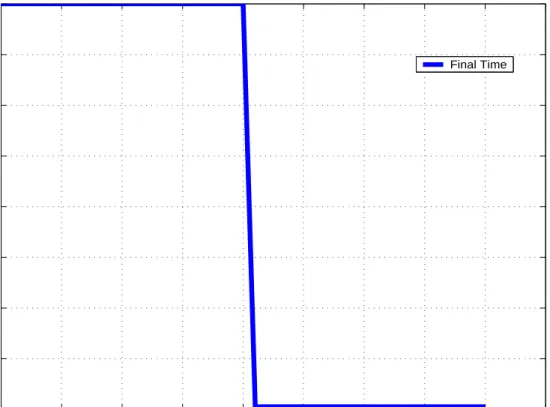
Looking at Figure 2.8 in detail, we can see that the change in the rendezvous times (i.e. tfi) starts at t = 2 and the control inputs are updated accordingly as obviously seen in Figure 2.7. Notice that same updating process is repeated at instants t = 4, 6, 8 until the rendezvous time t = 8.9062.
0 1 2 3 4 5 6 7 8 9 −2 0 2 4 6 8 10 12 14 16 time output Position 1 Position 2 Control Input1 Control Input 2
Figure 2.7: Position & control inputs vs. time for t0
i = 0, tfi = 10 in minimum energy control 0 1 2 3 4 5 6 7 8 9 8.8 9 9.2 9.4 9.6 9.8 10 time final time Final Time t f
Figure 2.8: Change in tf at communication instants for t0i = 0, tfi = 10 in
Chapter 3
APPLICATION TO
RENDEZVOUS PROBLEMS
In this chapter, we will present application results for the solution derived in Sec-tion 2.2.2 for more realistic problems like the multi-vehicle rendezvous problems in 1-D with fixed target (i.e. rendezvous point) and the multi-vehicle rendezvous problems with moving target in 2-D. In addition, the effect of imperfect commu-nication in the form of time delays will be discussed.
3.1
Multi-Agent Rendezvous Problem in 1-D
In this section, the application results for rendezvous problems in 1-D will be given. Moreover, time delays modeling late or lost rendezvous time information will be considered.
3.1.1
Three-Vehicle Rendezvous Problem
Let us consider the following dynamical model for a three-vehicle rendezvous problem: ˙xi = Aixi(t) + Bi(1 + wi(t))ui(t), t0 = 0, tf = 20, x1(t0) = 10 0 0 , x1(tf) = 0 0 0 , x2(t0) = 15 0 0 , x2(tf) = 0 0 0 , x3(t0) = 20 0 0 , x3(tf) = 0 0 0 , (3.1) where Ai = 0 1 0 0 0 1 0 0 0 , Bi = 0 0 1
and wi is an appropriate random signal accounting for imperfect road conditions or any other reason disturbing the cur-rent control input of the vehicle i. Vehicles are assumed to exchange information every 4 second and tfi is calculated as explained in Section 2.3.
In this model, the vehicles start at rest with zero acceleration and the input
ui(t) is used to control the rate of change in the acceleration. Furthermore, the
disturbances caused by the imperfect conditions (obstacles on the road, internal problems of the agents or other uncertainties) are included in the model as neg-ative or positive effects in the control input. These disturbances are handled by
wi(t) as random changes of ± 2 % in the optimal control input u∗i(t) during the
For this problem, Wc and u∗i(t) can be calculated at each communication
instant as indicated below. Note that, the formula for Wc and u∗i(t) are valid
until the next communication instant and are updated upon the next final time information. Wc = (1 2t20− t0t + 12t2)2 (12t20− t0t + 12t2)(t0− t) (12t20− t0t + 12t2 (1 2t20− t0t + 12t2(t0− t)) (t0− t)2 (t0− t) (1 2t20− t0t + 12t2) (t0− t) 1 ui(t) = −B1TeA T i(t0−t)W−1 c (x0i − eAi(t 0 i−t)xf i) (3.2)
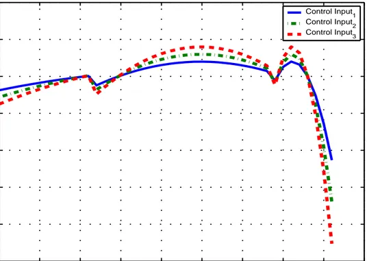
The simulation results for that problem are shown in Figures 3.1, 3.2 and 3.3. Recall that tf is determined as explained in Section 2.3. As seen in the figures,
the control inputs are updated when final time is updated, and the vehicles reach the rendezvous point simultaneously.
0 2 4 6 8 10 12 14 16 18 0 2 4 6 8 10 12 14 16 18 20 time position Position 1 Position 2 Position 3
Figure 3.1: Positions vs. time for rendezvous in 1-D without communication problems
0 2 4 6 8 10 12 14 16 18 −1 −0.8 −0.6 −0.4 −0.2 0 0.2 0.4 time control input Control Input 1 Control Input 2 Control Input 3
Figure 3.2: Control inputs vs. time for rendezvous in 1-D without communication problems 0 2 4 6 8 10 12 14 16 18 16 16.5 17 17.5 18 18.5 19 19.5 20 time final time Final Time
with-3.1.2
Three-Vehicle Rendezvous Problem in the Presence
of Communication Problems
Remember that the deficiencies in the information exchange were not considered in Section 3.1.1. Next, the communication problems are included in the problem statement in order to discuss the effects of late or missed information about the rendezvous times occurring during the task.
Let us begin with a simple but illustrative case assuming that the vehicles in the task force inform a central unit about their own final time, i.e. rendezvous instant, during the operation, the central unit determines the overall final time by finding the minimum of the final times, and informs all the vehicles in the task force back about the new rendezvous instant to reach the target point. In this case, it is assumed that the delays occur only in the information signals from the vehicles to the central unit, and not the other way around for simplicity.
In order to model the lost or late signals, it is reasonable for the central unit to specify a maximum delay hmaxand wait for all the information to be gathered.
If all the information comes before the maximum waiting time, then the central unit calculates the rendezvous time and informs all the vehicles. However, if there are still some missing information even though the maximum waiting time limit is reached, then the central unit calculates the rendezvous time assuming that the previous successful information is still valid for the vehicles that could not send their final time information. The reason for such an evaluation is simply the concern about the success of the mission, that even one of the vehicles cannot be at the rendezvous point on time, let the others be.
Thus, we have the following formulation for the final time tf
ta if(k) = tif(k) if hik ≤ hmax tif(k − 1) if hik > hmax tf(k) = min{ta1f(k), ta2f(k), . . . , taN f(k)} (3.3)
where
tf(k) : calculated final time at communication instant tk
ta
if(k) : assumed final time for vehicle i in the presence of time delay
tif(k) : final time for vehicle i to be transmitted to
the central unit in order to determine ta if(k)
hik : communication delay from vehicle i to the central unit
hmax : maximum delay limit applied by the central unit after which final
time is calculated and transmitted to the all vehicles in the task force
Note that hmax is chosen as 1 second and hiks are modeled as
hik ∼ |N(0, 0.9hmax)| (3.4)
i.e. we have normally distributed positive time delay values. Below are the sim-ulation results of the above configuration.
Instant(k) 1 2 3 4
Vehicle 1 19.9982 16.0275 16.0283 167.3708 Vehicle 2 14.0863 19.9977 16.0280 16.0277 Vehicle 3 20.0015 37.8605 16.0277 16.0277
Table 3.1: Calculated Final Time tf w.r.t. the communication instant
Instant(k) 1 2 3 4
Final time (sec) 14.0863 16.0275 16.0277 16.0277 Table 3.2: Final Times in the absence of time delays hiks
By looking at Table 3.1 and Table 3.2, we can see that the tif information
the minimum of these tifs. Since the effect of delay is not considered, there is no
deviation from the calculated values for tf. However, this is not the case when
the communication delay is taken into account as seen next.
Instant(k) 1 2 3 4
Vehicle 1 1.7243 0.0321 0.2711 0.8425 Vehicle 2 2.3702 1.0971 0.4884 0.0759 Vehicle 3 1.4989 0.6383 1.4527 0.7019
Table 3.3: Communication delays hik in sec. for corresponding instants k
In Table 3.3, we can see that some of the time delays hik are greater than the
threshold value hmax. That means the central unit will not be able to evaluate
the tif information coming from the corresponding vehicle and that will result in
a deviation from the calculated tf values in the absence of delay.
Instant(k) 1 2 3 4
Final time (without delay) 14.0863 16.0275 16.0277 16.0277 Final time (with delay) 20.0000 16.0275 16.0275 16.0275
Table 3.4: Final Times in the presence of time delays hiks
Looking at Table 3.1 and Table 3.4, we can see that at the first com-munication instant (i.e. k = 1) the final time tf should be 14.0863 since
it is the minimum of the tifs at that instant. However, as seen in Table
3.3, the time delays from the vehicles to the central unit are greater than
hmax and for that reason the central unit regards tifs as they did not change
w.r.t. their previous value, and accepts them as 20.0000 (ta
if(k)).
There-fore, tf is determined as min{20.0000, 20.0000, 20.0000} = 20 rather than
Similarly, the time delay h2k for vehicle 2 is greater than hmax in the second
communication instant. Even though this alters the flow of the algorithm, the final time result tf(k = 2) is not affected since min{16.0275, 19.9977, 37.8605}
and min{16.0275, 20.0000, 37.8605} give the same result as 16.0275.
In the last communication instant, time delay from vehicle 3 to the cen-tral unit is greater than hmax as seen in Table 3.3. Therefore, tfi(k =
3) is regarded as 16.0275, which is the previous value of it, and tf(k =
3) is determined as min{16.0283, 16.0280, 16.0275} = 16.0275 rather than min{16.0283, 16.0280, 16.0277} = 16.0277.
Now, let us take a look at the simulation results which are plotted in Fig-ures 3.4 - 3.8 0 2 4 6 8 10 12 14 16 18 0 2 4 6 8 10 12 14 16 18 20 time position Position 1 Position 2 Position 3
Figure 3.4: Positions vs. time for rendezvous in 1-D with one-way time delays in communication
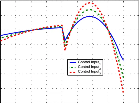
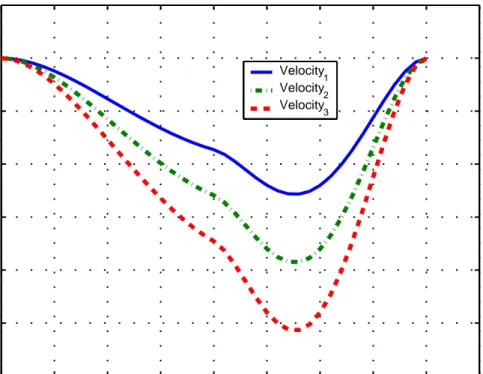
As seen in Figure 3.4, all of the 3 vehicles in the task force reach the ren-dezvous point at the same time, which means that the mission is completed successfully. Now, let us look at the trajectories of the other states (i.e. velocity and acceleration), the control input and the rendezvous time.
Looking at Figures 3.5-3.8, it can be observed that the only change in the final time, consequently the control input, the acceleration and the velocity, oc-curs just after t = 8 (to be precise t = 8.0321). That time instant is evidently
t(k = 2)+h12, the instant when the final time information of vehicle 1 is obtained.
0 2 4 6 8 10 12 14 16 18 −1 −0.8 −0.6 −0.4 −0.2 0 0.2 0.4 time control inputs Control Input 1 Control Input 2 Control Input 3
Figure 3.5: Control inputs vs. time for rendezvous in 1-D with one-way time delays in communication
0 2 4 6 8 10 12 14 16 18 −3 −2.5 −2 −1.5 −1 −0.5 0 0.5 time velocities Velocity 1 Velocity 2 Velocity3
Figure 3.6: Velocities vs. time for rendezvous in 1-D with one-way time delays in communication 0 2 4 6 8 10 12 14 16 18 −0.4 −0.2 0 0.2 0.4 0.6 0.8 1 time accelerations Acceleration1 Acceleration 2 Acceleration 3
Figure 3.7: Accelerations vs. time for rendezvous in 1-D with one-way time delays in communication
0 2 4 6 8 10 12 14 16 18 16 16.5 17 17.5 18 18.5 19 19.5 20 time rendezvous time Final Time
Figure 3.8: Change in tfis at communication instants for rendezvous in 1-D with one-way time delays in communication
Notice that, previously solved problem configuration is an illustrative exam-ple in order to see the flow of the algorithm in the case of time delays in the communication, and it should be improved in order to be much more realistic and applicable. Therefore, it is more reasonable to assume that the time delays are not just between the vehicles and the central unit, but rather between the vehicles. In other words, the vehicles in the task force send their final time in-formation not to the central unit but to each other, and each vehicle determines its individual final time accordingly. So, if the time delay hij from vehicle i to
vehicle j is greater than the acceptable limit whereas the time delay hji from
vehicle j to vehicle i is less than or equal to the limit, vehicle j cannot utilize the information coming from vehicle i while vehicle i can use the information sent from vehicle j. For that reason, the final time for each vehicle can be different
from the final times of the other vehicles and that can cause some deviations from the expected results.
Then, we have the following formulation for the final time tfi(k)
taif(k) = tif(k) if hij(k) ≤ hmax tif(k − 1) if hij(k) > hmax tfi(k) = min{ta1f(k), ta2f(k), . . . , taN f(k) (3.5) where
tfi(k) : final time to be used by vehicle i at tk
(determined upon receiving the information from the other vehicles)
tif(k) : calculated final time of vehicle i at tk
ta
if(k) : assumed final time for vehicle i due to the time delay
hij(k) : communication delay from vehicle i to vehicle j at tk
hmax : maximum delay limit applied by each vehicle after which
corresponding final time is calculated and used for completing the task
Note that hmax is chosen as 1 second and hij(k)s are modeled as in 3.4. The
simulation results of the explained configuration are presented next.
Instant(k) 1 2 3
Vehicle 1 20.0015 19.9960 22.9341 Vehicle 2 19.9985 19.9973 16.8726 Vehicle 3 20.0015 16.8714 15.3113
Instant(k) 1 2 3 Final time (sec) 19.9985 16.8714 15.3113
Table 3.6: Final Times in the absence of time delays hij(k)s
By looking at Table 3.5 and Table 3.6, we can see that the tif(k)
informa-tion would be processed at each communicainforma-tion instant and the tfi(k) would be determined by taking the minimum these tfi(k)s in the absence of time delays. However, as seen next, time delays between the vehicles will change the flow of the algorithm and the result.
h(1) = 0 0.2423 0.5864 0.5430 0 0.0178 0.6499 0.7575 0 h(2) = 0 0.7216 0.2115 0.6973 0 0.4059 0.7724 0.5591 0 h(3) = 0 0.3521 1.0979 0.3825 0 0.3672 1.8155 0.3548 0
Communication delays hij(k) for corresponding instants k are seen above (ij)th
entry of the corresponding 3x3 matrix represents the time delay from vehicle i to vehicle j). We can observe that some of the time delays hij are greater than
the threshold value hmax = 1 sec. For instance, the time delay from vehicle 3 to
vehicle 1 (i.e. h13(3)) at third communication is 1.0979 and the time delay from
vehicle 1 to vehicle 3 (i.e. h31(3)) at the same instant is 1.8155. That means
vehicle 1 will not be able to evaluate the final time information coming from vehicle 3 and vice a versa. This will result in a deviation from the final time
values calculated in the absence of delay.
Instant(k) 1 2 3
Vehicle 1 19.9985 16.8714 16.8714 Vehicle 2 19.9985 16.8714 15.3113 Vehicle 3 19.9985 16.8714 15.3113
Table 3.7: Final Times in the presence of time delays hij(k)s
Looking at Table 3.5 and Table 3.7, we can see that at third communication instant (i.e. k = 3) the final time tf(k = 3) should be 15.3113 since it is
the minimum of the tifs {22.9341, 16.8726, 15.3113}. However, the time delays
h13(3) and h31(3) are are greater than hmax and for that reason vehicles 1 and 3
determine their final times as tf1 = min{22.9341, 16.8726, 16.8714} = 16.8714 and
tf3 = min{19.9960, 16.8726, 15.3113} = 15.3113 by taking the previous final time informations of each other into account rather than the current ones. Therefore, vehicle 1 cannot be at the rendezvous point on time, whereas vehicles 2 and 3 can.
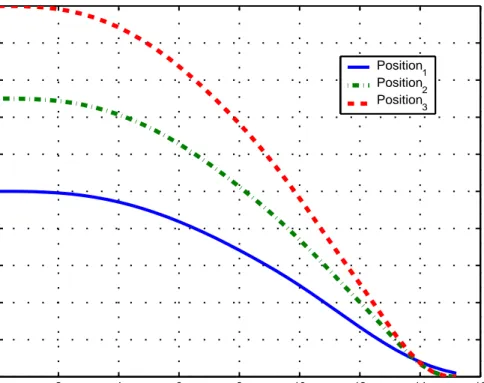
The simulation results are depicted in Figures 3.9-3.13. As seen in Figure 3.9, vehicles 2 and 3 meet at the rendezvous point on time whereas vehicle 1 is away from that point. Although that means the mission is not completed successfully, it can be said that the result is still satisfactory since vehicle 1 is very close to the rendezvous point.
0 2 4 6 8 10 12 14 16 0 2 4 6 8 10 12 14 16 18 20 time position Position 1 Position2 Position3
Figure 3.9: Positions vs. time for rendezvous in 1-D including communication problems 0 2 4 6 8 10 12 14 16 −3 −2.5 −2 −1.5 −1 −0.5 0 0.5 1 1.5 time control inputs Control Input 1 Control Input 2 Control Input 3
Figure 3.10: Control inputs vs. time for rendezvous in 1-D including communi-cation problems
0 2 4 6 8 10 12 14 16 −2.5 −2 −1.5 −1 −0.5 0 time velocities Velocity1 Velocity2 Velocity 3
Figure 3.11: Velocities vs. time for rendezvous in 1-D including communication problems 0 2 4 6 8 10 12 14 16 −0.4 −0.2 0 0.2 0.4 0.6 0.8 1 1.2 1.4 1.6 time accelerations Acceleration 1 Acceleration 2 Acceleration3
Figure 3.12: Accelerations vs. time for rendezvous in 1-D including communica-tion problems
0 2 4 6 8 10 12 14 16 15 15.5 16 16.5 17 17.5 18 18.5 19 19.5 20 time final time Final Time 1 Final Time 2 Final Time 3
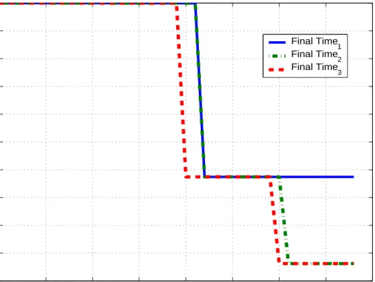
Figure 3.13: Change in tfis at communication instants for rendezvous in 1-D including communication problems
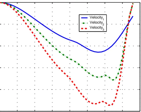
In Figures 3.14-3.18, results of another simulation is presented. Although the problem configuration is same as before, the effect of random disturbance wi(t)
is different. As seen in the plots, the vehicles reach the rendezvous point just at the same time, indicating that the mission is accomplished.
Instant(k) 1 2 3
Vehicle 1 20.0047 14.1826 14.1847 Vehicle 2 20.0046 19.9969 14.1848 Vehicle 3 20.0042 19.9969 14.1851
Instant(k) 1 2 3 Final time (sec) 20.0042 14.1826 14.1847
Table 3.9: Final Times in the absence of time delays hij(k)s
By looking at Table 3.5 and Table 3.6, we can see that the tif(k)
informa-tion would be processed at each communicainforma-tion instant and the tfi(k) would be determined by taking the minimum these tif(k)s in the absence of time delays.
However, as seen next, time delays between the vehicles will change the flow of the algorithm but not the results.
h(1) = 0 0.1265 0.7810 0.5896 0 0.8066 0.2932 0.5562 0 h(2) = 0 0.2583 0.7373 0.5576 0 1.0757 1.8981 0.2728 0 h(3) = 0 0.9126 0.2327 0.0312 0 0.5483 0.4585 0.9214 0
Communication delays hij(k) for corresponding instants k are seen above (ij)th
entry of the corresponding 3x3 matrix represents the time delay from vehicle i to vehicle j). We can observe that some of the time delays hij are greater than
the threshold value hmax. However, this does not change the calculation results
Instant(k) 1 2 3 Vehicle 1 20.0042 14.1826 14.1847 Vehicle 2 20.0042 14.1826 14.1847 Vehicle 3 20.0042 14.1826 14.1847
Table 3.10: Final Times in the presence of time delays hij(k)s
The plots of the simulation are presented next.
0 2 4 6 8 10 12 14 0 2 4 6 8 10 12 14 16 18 20 time position Position 1 Position2 Position3
Figure 3.14: Positions vs. time for rendezvous in 1-D including communication problems
As seen above, all of the vehicles meet at the rendezvous point on time which means that the mission is completed successfully.
0 2 4 6 8 10 12 14 −2.5 −2 −1.5 −1 −0.5 0 0.5 1 1.5 time control inputs Control Input 1 Control Input 2 Control Input 3
Figure 3.15: Control inputs vs. time for rendezvous in 1-D including communi-cation problems 0 2 4 6 8 10 12 14 −4 −3.5 −3 −2.5 −2 −1.5 −1 −0.5 0 time velocities Velocity 1 Velocity 2 Velocity 3
0 2 4 6 8 10 12 14 −1.5 −1 −0.5 0 0.5 1 1.5 2 time acceleration Acceleration 1 Acceleration 2 Acceleration 3
Figure 3.17: Accelerations vs. time for rendezvous in 1-D including communica-tion problems 0 2 4 6 8 10 12 14 14 15 16 17 18 19 20 21 time final time Final Time 1 Final Time 2 Final Time3
3.2
Multi-Agent Rendezvous Problem in 2-D
Naturally, a 2-D solution for the multi-agent rendezvous problem would be much more realistic than a 1-D solution for practical applications. Having obtained reliable solutions for the problem in 1-D, it is not so difficult to extend them to 2-D. The rendezvous problem in 2-D is divided into subproblems in 1-D on x and y axes, and they are solved as separate rendezvous problems in 1-D. Thus, at every communication instant we have two different expected final times for each vehicle as final times for x and y components of the states. Then, the minimum of the two is chosen as the expected arrival time for the corresponding vehicle and we proceed as explained in Section 2.3 to obtain the solution.Next, the solution results of the 2-D multi-agent rendezvous problem for fixed and moving target points are presented.
3.2.1
2-D Rendezvous Problem with Fixed Target
Let us consider the dynamic model below for the rendezvous problem in 2-D.
˙xi = Aixi(t) + Bi ³ ( h 1 1 i + wi(t)) · ui(t) ´ , t0 = 0, tf = 10 (3.6) where Ai = 0 1 0 0 0 1 0 0 0 , Bi = 0 0 1
and wi is an appropriate random signal accounting for imperfect road conditions or any other reason disturbing the cur-rent control input of vehicle i. Here, xi(t) and ui(t) are 3 × 2 and 1 × 2 matrices,
respectively and “·” denotes the element wise multiplication. It is assumed that
wi is in the form of
h
wix wiy
i