Selçuk J. Appl. Math. Selçuk Journal of Vol. 12. No. 1. pp. 77-93, 2011 Applied Mathematics
Application of a Numerical Method Using Radial Basis Functions to Nonlinear Partial Differential Equations
Marjan Uddin1, Sirajul Haq2
1University of Engineering and Technology, Peshawar, KPK, Pakistan
e-mail:m arjankhan1@ hotm ail.com
2Faculty of Engineering Sciences, GIK Institute, Topi, KPK, Pakistan
e-mail:sira j_ jcs@yaho o.co.in
Received Date: March 26, 2010 Accepted Date: May 26, 2011
Abstract. In this paper, we propose a meshfree method for numerical solution of various classes of partial differential equations (PDEs), such as the Boussinesq system, Drinefel’d-Sokolov-Wilson equations, and Hirota-Satsuma coupled KdV system. The meshfree algorithm is based on scattered data interpolation along with approximating functions known as radial basis functions (RBFs). The meshfree technique does not require space discretization. A set of scattered nodes provided by initial data is used for solution of the problem. Accuracy of the method is estimated in terms of the error norms 2, ∞, number of nodes in the domain of influence, time step size, parameter dependent and parameter independent RBFs, the numerical validation for the above mentioned three types of PDEs is given to check performance of the new approach.
Key words: RBFs; Partial differential equations; Boussinesq system; Drinefel’d-Sokolov-Wilson equations; Hirota-Satsuma coupled KdV system; Multiquadric (MQ), Quintics.
2000 Mathematics Subject Classification: 74S99. 1. Introduction and Preliminaries
Nonlinear PDEs describing wave propagation occur in fluid dynamics, plasma physics, solid-state physics, chemistry and mathematical biology [1, 21, 7,18]. Many authors have worked on the solution of coupled nonlinear evolution equa-tions using different techniques (see the references there in) [13, 6, 15, 2, 9, 12, 23].
The multiquadric method was introduced in 1971 by Hardy [8], which is based on scattered data approximation to approximate two-dimensional geographical surfaces. In 1990 Kansa [11] derived a modified multiquadric scheme for the numerical solution of PDEs. The existence, uniqueness, and convergence of the RBFs approximation was discussed by Micchelli [17], Madych [16], Frank and Schaback [3]. The importance of shape parameter in the MQ method was explained by Tarwater in 1985 [20]. Micchelli [17] has proved that for distinct interpolation points, the system of equations obtained by this method is always solvable. The idea of applying the MQ method to solve PDEs was proposed by Kansa [11], which was extended later on by Golberg [5]. Hon and Mao [10] extended the use of MQ method for the numerical solutions of various ordinary and partial differential equations including nonlinear Burgers equation with shock waves. Very recently Marjan Uddin and Sirajul Haq [14] have used (RBFs) to obtain meshfree numerical solution of time fractional PDEs.
In this paper, we propose a meshfree collocation method based on the radial basis functions, MQ (() = (2+ 2)12where is a shape parameter), and the spline basis Quintics (() = where is a positive odd integer) for solving the following classes of PDEs:
Class A: Boussinesq system [13]:
+ + + −6= 0 + + −2= 0 where is a small positive real parameter.
Class B: Drinefel’d-Sokolov-Wilson equations: + = 0
+ + + = 0 where , , , are arbitrary real constants.
Class C: Hirota-Satsuma coupled KdV system [13]: =
1
2− 3+ 3+ 3 = −+ 3
= −+ 3
The structure of the present paper is organized as follows. In Section 2, we discuss the meshfree method. In Section 3, we deal the stability analysis. Section 4, is devoted to the numerical tests of the method on the problems related to the Boussinesq system, Drinefel’d-Sokolov-Wilson equations and Hirota-Satsuma coupled KdV system. In Section 5, the results are concluded.
2. Analysis of the Method
In this section, we consider a general -dimensional ( = 1 2 3) time dependent boundary value problem
(1)
+ L = ( ) ∈ Ω B = () ∈ Ω
where L and B are derivative and boundary operators respectively. Ω and Ω represent domain and boundary of the domain respectively.
We use -weighted scheme for spatial derivatives in the following form: (2) (+1) − () + L (+1) + (1 − )L()= ( ()) + (1 − )( (+1)) In the above equation is time step, () ( is non-negative integer) is the solution at time ()= , 0 ≤ ≤ 1.
Let {}=1 and {}=+1be respectively interior and boundary points among
the collocation points {}=1 in the domain. The solution of Eq. (1) can be approximated by, (3) ()() = X =1 ()()
In the above eqution () are radial basis functions with Euclidean norm = k −k between the points and . {}=1are constants to be determined. From Eqs. (2) and (3), we can write:
(4) P =1 µ ()(+1) −()() + L [()] (+1) + (1 − )L [()] () ¶ = ( ()) + (1 − )( (+1)) = 1 2 (5) X =1 B(())(+1) = ( (+1)) = + 1
where = k− k. Eqs (4)-(5) are equations in unkhown {}=1, can be solved by using Gaussian elimination method. We use = 05 in our work. 2.1. Boussinesq system
Consider the Boussinesq system [13]:
(6) + + + −
6= 0 + + −2= 0
where is a real constant. The boundary conditions are:
(7) ( ) = 1() ( ) = 2() ( ) = 1() ( ) = 2() 0 and initial conditions
(8) ( 0) = () ( 0) = () ≤ ≤ From Eqs. (6), we can write
(9) h (+1)−() i +h− 2() (+1)− 2(1 − )() ()+ ( )(+1) +(1 − )()()+ ()()¤= 0 (10) h (+1) −() i +h− 6() ()+ ( )()+ n [()()()()+ ()()()() oi = 0 where (+1)= ()+ . In Eq. (9) the nonlinear term (
)(+1) is linearised as
()(+1)= (+1)() + ()(+1) − ()() . Using the above equation value of ()(+1)in Eq.(9) we obtain: (11)h (+1)−2()(+1)+ (()(+1) + (+1)() ) i = h ()+ 2(1 − )() ()− (1 − )()() + ()() − () i (12) h(+1)i=h()+ 6() () − () − (()()+ ()() ) i where () and ()are the th iterates of the approximate solutions. The RBFs approximation for the solutions and of Eq. (6) is given by: (13) ()() = X =1 ()1 () ()() = X =1 ()2 ()
Using Eq. (13), the system of Eqs. (11)-(12), along with the boundary condi-tions (7) can be written in matrix form:
(14) h A−2D3+ ²δtθ ³ u(n)∗ D 1+ u(n)x ∗ A ´i λ1(+1)= =£A+2(1 − )D3− (1 − )u(n)∗ D1+ u(n)∗ D1 ¤ λ1() − v(n)x + f(+1) (15) Aλ2(+1)= h A− (u(n)∗ D1+ u(n)x ∗ A) i λ2()+ 6u (n) xxx−u(n)x + g(+1) where ’*’ stands for component by component multiplication and
A= [()]=1 D1=£0()¤ =1 D3= £ 000()¤ =1, In more compact form we can write Eqs. (14)-(15) as:
(16) λ1 (+1)= M−1 1 N1λ1()+ M−11 F(+1) λ2(+1)= M−12 N2λ2()+ M−12 G(+1) where F(+1) = h1(+1) 0 0 2(+1)i − h()(1) 0 0 ()() i G(+1) = h1(+1) 0 0 (+1)2 i + 6 h ()(1) 0 0 ()() i − h() (1) 0 0 () () i M1= A −2D3+ ²δtθ(u(n)∗ D1+ u(n)x ∗ A) N1= A +2(1 − )D3− (1 − )u(n)∗ D1+ u(n)∗ D1
M2= A N2= A − (u(n)∗ D1+ u(n)x ∗ A) Eq. (13) can be written in matrix form as:
(17) u()= Aλ1() v()= Aλ2() Using Eq.(17) in Eq. (16), we get
(18) u
(+1)= AM−1
1 N1A−1u()+AM−11 F(+1) v(+1)= AM−1
2 N2A−1v()+AM−12 G(+1)
For distinct collocation points A is always invertible [17]. Invertibility of ma-trices M1 M2 are not always guaranteed.
2.2. Drinefel’d-Sokolov-Wilson equations
Here we consider the Drinefel’d-Sokolov-Wilson equations [19]:
(19) + + + = 0 + = 0
where , , , are arbitrary constants. The boundary conditions are given by: (20)
and initial conditions by:
(21) ( 0) = () ( 0) = () ≤ ≤
Using forward difference time derivative and -weighted RBFs approximation for spatial derivative as given in Eq. (2), Eqs. (19) lead to the following set of equations. (22) (+1)= ()− ()() and (23) (+1)+ 2 (+1) = ()− 2 () − ()() − () () We adopt the same procedure as given in subsection 2.1 to find the solution of the system (19)-(21).
2.3. Hirota-Satsuma coupled KdV system
The Hirota-Satsuma coupled KdV system [13] is given by:
(24)
= 12− 3+ 3+ 3 = −+ 3
= −+ 3 with boundary conditions:
(25) ( ) = 1() ( ) = 2() ( ) = 1() ( ) = 2() ( ) = 1() ( ) = 2()
0
The initial conditions for the above system are given by:
(26) ( 0) = () ( 0) = () ( 0) = () ≤ ≤ : Using the rules (2) in Eqs. (24), we obtain
(27) (+1) −4(+1) + 3 2( (+1)() + ()(+1) ) = ()+ 4 () +3(()() + ()() ) (28) (+1)+ 2 (+1) = ()− 2 () + 3()() and (29) (+1)+ 2 (+1) = ()− 2 () + 3()()
System of equations (27)-(29) is solved by using the same procedure given in the subsections 2.1 and 2.2.
3. Stability of the Scheme
In this section, we discuss the stability analysis for the scheme (18), by using spectral norm of the amplification matrix. We assume that u, v be numerical and u∗, v∗ be exact solutions of Eq. (6). The error vectors ε(n)
i ( = 1 2) are defined by ε(n)1 = u()− u∗(), ε(n)
2 = v()− v∗(). Putting values from Eq. (18) in these equations, we arrive at the following equations:
(30) ε
(n+1)
1 = u(n+1)− u∗(+1)= AM−11 N1A−1ε(n)1 = E1ε(n)1 ε(n+1)2 = v(n+1)− v∗(+1)= AM−1
2 N2A−1ε(n)2 = E2ε(n)2
where E1 = AM−11 N1A−1 and E2 = AM−12 N2A−1 are the amplification matrices. For the scheme to remain stable, ε(n)i must approach to 0, (for i=1,2) as −→ ∞ (E1) ≤ 1, (E2) ≤ 1 which is necessary and sufficient condition of stability, where (E1) and (E2) represent spectral radii of the matrices E1 and E2 respectively. From Eqs. (16) and (30), we can write:
(31) [I + P1] ε (n+1) 1 = [I + (2)P2] ε (n) 1 [I] ε(n+1)2 = [I + (2)Q2] ε(n)2 where P1 = h −2D3+ ²(u(n)∗ D1+ u(n)x ∗ A) i A−1 P2 = h (1 − )D3− 2(1 − )u(n)∗ D1+ 2u(n)∗ D1 i A−1 Q2 = h −2(u(n)∗ D1+ u(n)x ∗ A) i A−1 For stability, the maximum eigenvalues of the matrices
[I + P1]−1[I + (2)P2] and [I + (2)Q2] must be less than unity or equivalently we can say that
(32) ¯ ¯ ¯ ¯ 1 + (2)2 1 + 1 ¯ ¯ ¯ ¯ ≤ 1 and ¯¯1 + (2)2 ¯ ¯ ≤ 1
where 1, 2 and 2 stand for eigenvalues of the matrices P1, P2, and Q2 respectively. When =1
2, the conditions (32) reduce to: (33) ¯ ¯ ¯ ¯ 1 + (2)2 1 + (2)1 ¯ ¯ ¯ ¯ ≤ 1 and ¯¯1 + (2)2 ¯ ¯ ≤ 1
Above conditions will hold if 1 ≥ 2. In case when = 0, (32) give (34) ¯¯1 + (2)2 ¯ ¯ ≤ 1 and ¯¯1 + (2)2 ¯ ¯ ≤ 1
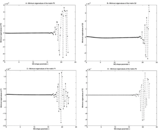
It is evident from inequality (32), that the stability of the scheme (18) depends upon the parameters , and eigenvalues of the matrices P1 P2 Q2. In the case of free shape parameter RBFs like TPS and Quintics, eigenvalues depend on a number of collocation points only. For an acceptable distribution of collocation points, inequality (32) must hold. In the case of RBFs with shape parameter like MQ, stability depends upon shape parameter as well. We in-vestigate influence of the parameter numerically when remains constant. In Table 4, we have shown minimum eigenvalues of the matrices M1 M2. It is noted that eigenvalue of these matrices remain constant in the region of conver-gence. In this region the inequalities (33)-(34) are satisfied as shown in Fig. 3. In such RBFs the condition numbers and the magnitudes of the eigenvalues of the matrices P1 P2 Q2are closely related to the shape parameter . We have analyzed dependence of stability on the shape parameter numerically which is shown in Table 4 and Fig. 3, by keeping fixed. It is clear from the Table 4 that the accuracy of RBFs approximations can be improved by changing value in the interval (005 2234) where the solution remain stable. As ≥ 2234 the condition numbers of the matrices Q1 Q2 P1 P2 become so large that the system of linear equations become ill-conditioned, thus producing unstable solution.
4. Numerical Examples
In this section, we apply the proposed method for the numerical solution of different classes of coupled PDEs. The accuracy of the meshfree method is tested in terms of 2 and ∞ error norms. These error norms are defined as:
2= k∗− k2= ⎡ ⎣ X =1 (∗− )2 ⎤ ⎦ 12 (35) ∞= k∗− k∞= max|∗− | The tested problems are given below.
Problem 1. Consider the Boussinesq system (6) with the exact solutions given in [13] (36) ( ) = 4 2(1 − 2)(3p(1 − 22)(1 − 223)) ( ) = 42 ( )(1 − 2)(3(1 − 22)(1 − 223)) where ( ) = (1 − 423 − 2323 + 3) + 2(−3 + 23 + 22)
= tanh(( − )) =p(1 − 22)(1 − 223)
The initial and the boundary conditions (8)-(9) are extracted from the exact solutions (36).
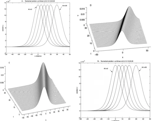
The error norms ∞and 2of the meshfree method are given in Table 1. These numerical results are obtained by MQ method for = 01 001, = 01 = −20 = 20 = 21 shape parameters 1= 2= 05 using different values of . We compare our results with those obtained in [13] which are listed in Table 2. From the comparison of Tables 1 and 2 it follows that the present method produces better results to those given in [13]. Solitary waves solutions and are shown in Figs. 1() and 1() respectively, initially centered at = 0 and moving from left to right with constant speed . In Table 3, we list amplitudes of the two waves and up to time 30. It is clear from the Fig. 1 and Table 3 that amplitudes of the two solitary waves and are nearly constant at different times, showing the conservative nature of the RBFs approximations at different time levels.
Figure 1. Stability graph of numerical solutions and respectively at time = 0 : 5 in the domain [−20 20], Figs 3A-3B depicted for the value
= 0 while for Figs 3C-3D we use =: 5 where = 0 : 01; = 0 : 01; = 0 : 001; = 2; corresponding to the Problem 1.
Figure 2.Plots of the solutions, when = 001, = 01, = 1, = 0001, 1= 0025, 2= 0025. Figs.1(A)-1(B) show the motion of the solitary waves and moving from left to right, initially centered at = 0 at times
= 0, 5, 10, 15, 20, 30. Figs.1(C)-1(D) represents the exact and numerical solutions and at time = 0, 30 in [−50 50], corresponding to of Problem 1.
Problem 2. In this problem we consider the Drinefel’d-Sokolov-Wilson equa-tions (24) with the exact soluequa-tions [19]
(37) ( ) = 2 sec 2( − ) ( ) = 2 sec ( − )
In this case the initial and boundary conditions (25) and (26) are derived from the exact solutions (37).
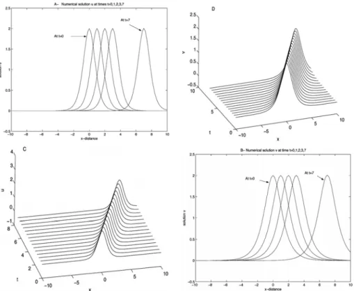
In Table 5, absolute error between the exact and numerical solutions for = 0001 = −10 = 10 = 101 MQ shape parameters 1= 11 2 = 11. In Figs. 2() and 2() solitary waves solutions and , initially centered at = 0 moving from left to right with the constant speed 1 are shown. In Table 6 amplitudes of the two waves and up to time 7 are listed. It is clear from Fig. 2 and Table 6, that amplitudes of the two solitary waves and are nearly constant at different times, showing the accuracy and stability of the RBFs approximations at different time levels.
Figure 3.Plots of the solutions, when = 1, = 0001, 1= 11, 2= 11. Figs.2(A)-2(B) show the motion of the solitary waves and moving from left
to right, initially centered at = 0 at times = 0 1 2 3 7 in [-10,10], corresponding to Problem 2.
Problem 3. Finally we consider the Hirota-Satsuma coupled KdV system with the exact solutions [13]:
(38) ( ) = 42 2tanh2() − 8223 − 3 ( ) = 222tanh2() − 2223 − 43 − 0 ( ) = 22 2tanh2() − 222+ 0 where =√2( − ) and ≤ ≤
The boundary and the initial conditions are obtained from the exact solutions (38).
In Tables 7 and 8, the error norms ∞and 2are presented. These numerical results are obtained by the present (MQ) and Quintics (7) methods. The results are given for = −30 = 30 = 01 0 = 01 2 = 01 MQ shape parameters 1 = 025 = 2 = 025 and different values of and time . The results are compared with the results obtained in [13] are listed in Table 9. From the comparison of Tables 7-9 it follows that the present methods produces better results.
5. Concluding Remarks
In this paper, a meshfree interpolation method using radial basis functions is applied for the solution of system of nonlinear evolution equations. The per-formance of this method is in excellent agreement with exact solution and with
results given in [13]. We have established the stability analysis of the method. The technique used in this paper provides an efficient alternative for the solution of nonlinear partial differential equations. Contrary to the traditional methods, like FDM and FEM, this approach is meshfree and accuracy of the method can be increased by varying value of shape parameter, while keeping number of collocation points fixed. It is noted that time marching process reduces the so-lution accuracy due to the time truncation errors. From application viewpoints the implementation of this method is very simple and straightforward.
6. Acknowledgements
The first author is thankful to HEC Pakistan for financial help through Grant No. 063-281079-Ps3-169.
References
1. R. Davidson, Methods in Nonlinear Plasma Theory, Academic Press, New York, 1972.
2. E. Fan, Soliton solutions for a generalized Hirota-Satsuma coupled KdV equation and a coupled MKdV equation, Phys. Lett. A. 282 (2001) 18-22.
3. C. Franke, R. Schaback, Convergence order estimates of meshless collocation meth-ods using radial basis functions, Adv. Comput. Math. 8 (1998) 381-99.
4. D. D. Ganji, M. Jannatabadi, E. Mohseni Application of He’s variational iteration method to nonlinear Jaulent-Miodek equations and comparing it with ADM, Phycs. Lett. A. 299 (2006) 201-206.
5. M. A. Golberg, C. S Chen, S. R. Karur, Improved multiquadric approximation for partial differential equations, Engng. Anal. Bound. Elemt. 18 (1996) 9-17.
6. G. Gottwald, R.Grimshaw, B. Malomed, Parametric envelope solitons in coupled KdV equations, Phys. Lett. A 227 (1997) 47-54.
7. P. Guy, S. Scott, Chemical Osillations and instabilities, Clarendon Press, Oxford, 1990.
8. R.L. Hardy, Multiquadric equations of topography and other irregular surfaces, Geo. Phycs. Res. 176 (1971), 1905-1915.
9. R. Hirota, J. Satsuma, Soliton solutions of a coupled Kortewege-de Vries equation., Phys. Lett. A. 85 (1981) 407-408.
10. Y. C. Hon, X. Z. Mao, An efficient numerical scheme for burgers equation, Appl. Math. Comput. 95 (1998) 37-50.
11. E. J. Kansa, Multiquadrics scattered data approximation scheme with applications to computational fluid-dynamics I, surface approximations and partial derivative esti-mates, Comput. Math. Appl. 19 (1990) 127-145.
12. D. Kaya, E. Ibrahim. Inan, Exact and numerical traveling wave solutions for nonlinear coupled equations using symbolic computation, Appl. Math. Comput. 151 (2004) 775-787.
13. A. H. Khater, R. S. Temsah, D. K. Callebaut, Numerical solutions for some coupled nonlinear evolution equations by using spectral collocation method, Math. Comput. Model., 48 (2008) 1237-1253.
14. A. H. Khater, W. Malfliet, E. S. Kamel, Travelling wave solutions for of some classes of nonlinear evolution equations in (1+1) and higher dimensions, Math. Com-put. Simulation, 64 (2004) 247-258.
15. W. R. Madych, S. A. Nelson, Multivariate interpolation and conditionally positive definite functions II, Math. Comput. 54 (1990) 211-30.
16. Marjan Uddin, Sirajul Haq, RBFs approximation method for time fractional par-tial differenpar-tial equations, Commun. Nonlinear Sci. Numer. Simulat. doi:10.1016/j. cnsns.2011.03.021
17. C. A. Micchelli, Interpolation of scatterted data: distance matrix and conditionally positive definite functions Construct. Approx., 2 (1986) 11-22.
18. J. Muray, Mathematical Biology, Springer, Berlin, 1981.
19. A. A. Soliman, M. A. Abdou Numerical solutions of nonlinear evolution equations using variational iteration method, J. Comput. Appl. Math. 207 (2007) 111-120. 20. A.E. Tarwater, A parameter study of Hardy’s multiquadric method for scat-tered data interpolation, Lawrence Livermore National Laboratory, Technical Report UCRL-54670, (1985).
21. M. Toda, Studies of a Nonlinear Lattice, Springer, Berlin, 1981.
22. Yan Xu, Chi-Wang Shu, Local discontinuous Galerkin methods for the Kuramoto-Sivashinsky equations and the Ito-type coupled equations, Comput. Methods. Appl. Mech. 195 (2006) 3430-3447.
23. Z. Zhengdi, B. Qinsheng, W. Jianping, Bifurcations of travelling wave solutions for two coupled variant Boussinesq equations in shalow water waves, Chaos Solitons Fractals 24 (2005) 631-643.