Selçuk J. Appl. Math. Selçuk Journal of Vol. 8. No.1. pp. 45-49 , 2007 Applied Mathematics
Solving nonlinear fifth-order boundary value problems by differential transformation method
Vedat Suat Erturk
Department of Mathematics, Faculty of Arts and Sciences, Ondokuz Mayis University, 55139, Samsun, Turkey.
e-mail:dsim sek@ selcuk.edu.tr
Received : December 25, 2006
Summary. In this study, we implement differential transformation method (DTM) for solving nonlinear fifth-order boundary value problems arising in vis-coelastic flows. A numerical example is presented to illustrate the efficiency and reliability of this method.
Key words: Fifth-order boundary value problems, differential transformation method, numerical solution
1. Introduction
In this work, we consider a fifth-order boundary value problem of the form
(1.1) (5)() = ( ) 0 subject to the boundary conditions
(1.2) (0) = 0 0(0) = 1 00(0) = 2 () = 0 0() = 1
where is ( ) is a given continuous, nonlinear function of = () and ( =
0 1 2), and ( = 0 1) are real finite constants [1].
Such problems arise in the mathematical modeling of viscoelastic flows [2,3]. Theorems which list the conditions for the existence and uniqueness of solutions of this types of problems are thoroughly discussed; see Agarwal [4].
In [2,3], two numerical algorithms,namely,spectral Galerkin methods and spec-tral collocation methods were applied to address the numerical issues related
to such problems. Moreover, Khan [5] and Wazwaz [6] investigated these prob-lems by using the finite-difference methods and decomposition method, respec-tively.Recently, Caglar et al.[1], Siddiqi and Akram[7] investigated the fifth order boundary value problems using spline functions.
In the present paper, differential transformation method has been used to solve fifth-order boundary value problems which are assumed to have a unique solu-tion in the interval of integrasolu-tion [4]. The concept of differential transform was first introduced by Zhou [8], in a study about electric circuit analysis. It is a semi-numerical-analytic-technique that formulizes Taylor series in a totally dif-ferent manner. With this technique, the given differential equation and related boundary conditions are transformed into a recurrence equation that finally leads to the solution of a system of algebraic equations as coefficients of a power series solution.
2. Differential transformation method
The differential transformation of the th derivative of a function () is as follows: (2.1) () = 1 ! ∙ () ¸ =0 and the inverse differential transformation is defined as
(2.2) () =
∞
X
=0
()( − 0)
The following theorems that can be deduced from Eqs. (2.1) and (2.2) are given below:
In actual applications, function () is expressed by a finite series and Eq. (2.2) can be written as (2.3) () = X =0 ()( − 0)
Eq. (2.3) implies thatP∞=+1 ()( − 0) is negligibly small. In fact, is
decided by the convergence of natural frequency in this study. Theorem 1If () = () ± ()then () = () ± ()
Theorem 2If () = ()then () = ()where is a constant. Theorem 3If () = () then () =
(+)!
Theorem 4If () = ()()then () =P1=0(1)( − 1)
Theorem 5If () = then () = (−) where, (−) = ½
1 = 0 6= 3. Numerical results
Example 3.1.Consider the following boundary value problem (3.1) (5)() = −2() 0 1
subject to the boundary conditions
(3.2) (0) = 0(0) = 00(0) = 1 (1) = 0(1) =
Theoretical solution for this problem is
(3.3) () =
Knowing that the differential transformation of −is (−1)! and using
The-orems 3 and 4, Eq. (3.1) is transformed as follows:
(3.4) ( + 5) = 1 (+1)(+2)(+3)(+4)(+5)× P 2=0 P2 1=0 (−1)−2 (−2)! (1) (2− 1)
By using Eqs.(2.1) and (3.2), the following transformed boundary conditions at 0= 0 can be obtained: (3.5) (0) = 1 (1) = 1 (2) = 1 2 X =0 () = and X =1 () = where, is a sufficiently large integer. By using the inverse transformation rule in Eq.(2.2), for = 7, we get
(3.6) () = 1 + + 2 2 + 3+ 4+ 5 120 + 6 720+ 7 5040+ ( 8)
where, according to Eq.(2.1), = 000(0)
3! = (3) and = (4)(0)
4! = (4)
We can obtain the following system of equations from the fourth and fifth equal-ities in Eq. (3.5) :
(3.7) + = −
1265 504
3 + 4 = − 1477720
This in turn gives
(3.8) = 01665518346 and = 00418093590 Accordingly, we get the following series solution
(3.9)
() = 1 + + 052+ 016655183463+ 004180935904
+ 000833333335+ 000138888896+ 000019841277
+ (8)
By continuing the same procedure for = 13, we get the following series solu-tion: (3.10) () = 1 + + 052+ 016666666653+ 004166666684 + 000833333335+ 000138888896+ 000019841277 + 000002480168+ 000000275579+ 0000000275610 + 0000000025111+ 0000000002112+ 000000000013 + (14)
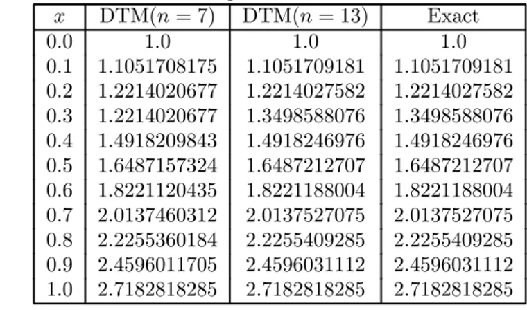
Numerical results for = 7 and = 13 with the comparison to the exact solution () = are given in Table 1.
Table 1: Numerical results compared to the exact solution for Example 3.1. DTM( = 7) DTM( = 13) Exact 00 10 10 10 01 11051708175 11051709181 11051709181 02 12214020677 12214027582 12214027582 03 12214020677 13498588076 13498588076 04 14918209843 14918246976 14918246976 05 16487157324 16487212707 16487212707 06 18221120435 18221188004 18221188004 07 20137460312 20137527075 20137527075 08 22255360184 22255409285 22255409285 09 24596011705 24596031112 24596031112 10 27182818285 27182818285 27182818285
As one can see from Table 1, the results obtained with the differential trans-formation method for = 13 are ten digits accurate. Also, as the number of terms involved increase, one can observe that the series solution obtained by
the differential transformation method converges to the series expansion of the exact solution () = .
4. Conclusion
Differential transformation method (DTM) was applied to the nonlinear fifth-order boundary value problems. The study showed that this method is simple and easy to use and produces reliable results.
References
1. H.N. Caglar, S.H. Caglar, E.H. Twizell, The numerical solution of fifth-order boundary-value problems with sixth-degree B-spline functions, Appl. Math. Lett. 12 (1999) 25—30.
2. A.R. Davis, A. Karageorghis, T.N. Phillips, Spectral Galerkin methods for the primary two-point boundary-value problem in modeling viscoelastic flows, Internat. J. Numer. Methods Eng. 26 (1988) 647—662.
3. A.R. Davis, A. Karageorghis, T.N. Phillips, Spectral collocation methods for the primary two-point boundary-value problem in modelling viscoelastic flows, Internat. J. Numer. Methods Eng. 26 (1988) 805—813.
4.R.P. Agarwal, Boundary Value Problems for High Ordinary Differential Equations, World Scientific, Singapore, 1986.
5.M.S. Khan, Finite-difference solutions of fifth-order boundary-value problems, Ph.D. Thesis, Brunel University, England, 1994.
6. A.M.Wazwaz, The numerical solution of fifth-order boundary value problems by the decomposition method, J.Comput.Appl.Math. 136(2001) 251-261.
7.S.S. Siddiqi, Ghazala Akram, Sextic spline solutions of fifth order boundary value problems, Appl. Math. Lett., 20 (2007), 591-597.
8.J. K. Zhou, Differential Transformation and Its Applications for Electrical Circuits (in Chinese), Huazhong Univ.Press, Wuhan. China, 1986