Selçuk J. Appl. Math. Selçuk Journal of Special Issue. pp. 35-52, 2011 Applied Mathematics
Mixture Distribution Model Approximation to System Reliability Ayça Hatice Türkan1, Hamza Erol2
1Department of Statistics, Faculty of Science and Literature, Afyon Kocatepe
Univer-sity, 03200 Afyonkarahisar, Turkiye e-mail: aturkan@ aku.edu.tr
2Department of Statistics, Faculty of Science and Literature, Çukurova University,
01330 Adana, Turkiye e-mail: herol@ m ail.cu.edu.tr
Abstract. In this study, mixture reliability functions, mixture probability density functions and mixture hazard functions were established for reliabil-ity block diagrams of series, parallel and complex systems. Mixture reliabilreliabil-ity function, mixture probability density function and mixture hazard function, es-tablished for systems studied, were proposed as an approximation to reliability function, probability density function and hazard function respectively. It was shown that system reliability functions, system probability density functions and system hazard functions can be expressed in terms of component reliability functions, component probability density functions and component hazard func-tions respectively. By the mixture distribution model approximation to system reliability: function representations were simplified, function calculations were decreased and information extracted from the system and its components were increased for reliability block diagrams of series, parallel and complex systems. Key words: Component reliability, Hazard function, Mixture probability den-sity function, Reliability block diagram, Reliability function, Statistical reliabil-ity analysis, System reliabilreliabil-ity.
2000 Mathematics Subject Classification: 62N05. 1. Introduction
Estimating the reliability of a system and its components is one of the major problems in statistical reliability analysis [4]. Reliability of the product can be defined as the probability that the product continues to meet the specifica-tion over a given time period subject to given environmental condispecifica-tions [1,2]. Discrete distributions are used to model discrete events such as the number of errors that occur in a specific time frame. Continuous distributions are used to model variables that have real values such as time to failure [12].
Probability distributions are widely used for system failure distributions or com-ponent failure distributions [2,6]. Lifetime of a system depends on many factors such as amount of production, substance used in production or changes in envi-ronmental conditions. In statistical reliability analysis, time for system is taken as a random variable and then an appropriate probability model is designed for failure times of system. Parameters are estimated in the probability models. Some properties of probability models such as the reliability function and the hazard function are reviewed [10]. A multi-component system consists of at least two components in series or at least two components in parallel or com-binations of these. The structure of a multi-component system is indicated by a reliability block diagram. A system is a collection of components arranged according to a specific design in order to achieve desired functions with accept-able performance and reliability measures [5]. The type, the quality and the design of the components have a direct effect on the system performance and system reliability. Reliability block diagram of a system considered should be established in the first step to determine the reliability of that system [11]. Re-liability block digram is a graphical representation of the system’s structure [5]. A block represents a component or a subsystem of the system.
In this study, mixture reliability functions, mixture probability density functions and mixture hazard functions were established for reliability block diagrams of series, parallel and complex systems. Mixture reliability function, mixture prob-ability density function and mixture hazard function, established for systems studied, were proposed as an approximation to reliability function, probability density function and hazard function respectively. It was shown that system reliability functions, system probability density functions and system hazard functions can be expressed in terms of component reliability functions, compo-nent probability density functions and compocompo-nent hazard functions respectively. By the mixture distribution model approximation to system reliability: func-tion representafunc-tions were simplified, funcfunc-tion calculafunc-tions were decreased and information extracted from the system and its components were increased for reliability block diagrams of series, parallel and complex systems.
2. Method
A mixture distribution model is defined as finite sum of weighted at least two component (pure) distribution models. Mixture distribution models arise when the population of interest contains two or more subpopulations. A component of the system may fail at different times according to other. Environmental effects or conditions of use are the factors affecting the lifetime distributions for the system or its components. When a homogeneous population of products is oper-ated at different conditions, the life of the products usually has multiple modes. This situation brings to mind the finite mixture distribution. It is difficult to distinguish the non-homogeneous populations and analyze them individually. For example; automobiles, having the same type, having the same features and produced at the same fabric, sold do continue operation with different life times
in different locations. Then mixture of vehicles in different locations arises. In this situation, a finite mixture distribution is useful [13]. Because of the characteristics of components, lifetime distributions of systems have variety and therefore frequently can not be approximated by simple distribution functions. Bucar et al. (2004), proved that the reliability of an arbitrary system can be approximated well by a finite Weibull mixture without knowing the structure of system. They studied parameter estimation of unknown parameters of mixture distribution model.
Finite mixture models were proposed as an approximation to probability density functions of systems. A lifetime distribution of a system can be defined by (1) f (tj; θ) =
g X i=1
pifi(tj; ψi), tj > 0, j = 1, 2, . . . , n
where tj for j = 1, 2, . . . , n is the random variable; θ = (pi, Ψi) for i = 1, 2, . . . , g is the vector containing all the parameters in probability density function for the system; pi’s are the mixing proportions or weighting factors such that 0 < pi< 1 andPgi=1pi= 1; fi(tj; ψi)’s are component density functions for the system and ψi for i = 1, 2, . . . , g is the vector containing the parameters in the component density functions [3,9].
In this study, we propose a method of computing statistically system reliability and system risk for reliability block diagrams of series, parallel and complex sys-tems using mixture distribution models. For this purpose mixture distribution models have been established for reliability block diagrams of series, parallel and complex systems. The distribution of each component in mixture distribu-tion model for reliability block diagrams of series, parallel and complex systems is assumed to be a Weibull distribution. A random variable t has a Weibull distribution if its probability density function is
(2) fi(tj; αi, βi) = βi αi µ tj αi ¶βi−1 exp " − µ tj αi ¶βi# , tj > 0, αi> 0, βi> 0 for i = 1, 2, . . . , g. Where αi and βi parameters of Weibull distribution are scale and shape parameters respectively [8]. Therefore, the probability density function for reliability block diagrams of series, parallel and complex systems is (3) f (tj; pi, αi, βi) =
Pg
i=1pifi(tj; αi, βi) , tj> 0, αi> 0, βi > 0, 0 ≤ pi≤ 1, Pgi=1pi= 1
Thus the mixture of two parameter Weibull distributions is as the lifetime dis-tribution model.
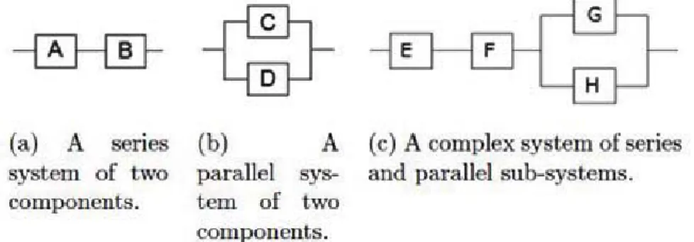
The reliability block diagrams of the systems considered is shown in Figure 1. In this study reliability functions, probability density functions and hazard
functions will be established for reliability block diagrams of series, parallel and complex systems. Then mixture reliability functions, mixture probability den-sity functions and mixture hazard functions will be established for reliability block diagrams of these systems. After then reliability functions will be com-pared with the mixture reliability functions, probability density functions will be compared with mixture probability density functions and hazard functions will be compared with mixture hazard functions. Systems, shown in Figure 1, considered in this study are prototype systems.
The distribution of each component and the parameters of components are as-sumed to be known as: component A has Weibull (t;1000,1.5) distribution, component B has Weibull (t;10000,1.5) distribution in reliability block diagram of series system in this study. The distribution of each component and the parameters of components are assumed to be known as: component C has Weibull (t;8000,10) distribution, component D has Weibull (t;5000,4) distrib-ution in reliability block diagram of parallel system in this study. The distri-bution of each component and the parameters of components are assumed to be known as: component E has Weibull (t;1000,1.5) distribution, component F has Weibull (t;10000,1.5) distribution, component G has Weibull (t;1000,3) distribution, component H has Weibull (t;5000,1.5) distribution in reliability block diagram of complex system in this study.
Figure 1. The reliability block diagrams of the systems considered. Reliability functions and mixture reliability functions, probability density func-tions and mixture probability density funcfunc-tions, hazard funcfunc-tions and mixture hazard functions will be established for reliability block diagrams of series, par-allel and complex systems. First the reliability function Rs(t) will be defined for the reliability block diagram of the systems studied. Then the probability density function fs(t) will be obtained from the reliability function Rs(t) of the systems studied. After then the hazard function hs(t) will be computed by using the probability density function fs(t) and the reliability function Rs(t) of the systems studied. Finally the mixture reliability function Rsmixture(t), the mix-ture probability density function fsmixture(t) and the mixture hazard function hmixture
Generating data set for failure times of series system in Figure 1a: First the data is generated from each component distribution. Then, the minimum value of failure times of each generation for component A and component B is selected. Process is repeated 10000 times. Each time, the number of failures caused by each component is counted. The mean of the number of failures for each component is divided by the number of the failures of the system. So, mixing proportion or weighting factor of each component is obtained. Generating data set for failure times for parallel system in Figure 1b: First the data is generated from each component distribution. Then, the maximum value of failure times of each generation for component C and component D is selected. Process is repeated 10000 times. Each time, the number of failures caused by each component is counted. The mean of the number of failures for each component is divided by the number of the failures of the system. So, mixing proportion or weighting factor of each component is obtained. Generating data set for failure times for complex system of series and parallel sub-systems in Figure 1c: First the data is generated from each component distribution. Then, the maximum value of failure times of each generation for component G and component H, and the minimum value of failure times of each generation for component E and component F are compared. Then the minimum is selected. Process is repeated 10000 times. Each time, the number of failures caused by each component is counted. The mean of the number of failures for each component is divided by the number of the failures of the system. So, mixing proportion or weighting factor of each component is obtained.
2.1. Case 1: A Series System of Two Components
For Case 1, the reliability block diagram of a series system with two components is shown in Figure 1a. The reliability function Rs(t) for the series system with two components is defined by
(4) Rs(t) = RA(t)RB(t), t > 0
where RA(t) and RB(t) are the reliability functions of the components A and B respectively. The probability density function fs(t) for the series system with two components can be obtained from reliability function Rs(t) for the series system with two components by
(5) fs(t) = −
∂Rs(t) ∂t , t > 0
Then the probability density function fs(t) for the series system with two com-ponents can be expressed as
(6) fs(t) = fA(t)RB(t) + fB(t)RA(t), t > 0
where fA(t) and fB(t) are the probability density functions of the components A and B respectively. The hazard function hs(t) for the series system with two
components can be computed by using,
(7) hs(t) =
fs(t) Rs(t)
, t > 0.
Let’s generate 100 data from Weibull (t;1000,1.5) distribution for component A in reliability block diagram of series system in Figure 1a. Let’s denote the elements of this data set as tA1, tA2, . . . , tA100. Let’s generate 100 data from
Weibull (t;10000,1.5) distribution for component B in reliability block diagram of series system in Figure 1a. Let’s denote the elements of this data set as tB1, tB2, . . . , tB100. Let’s take tk = min (tAk, tBk) for k = 1, 2, . . . , 100. Let’s
denote the number of counts tk from component A as nA and from compo-nent B as nB. Thus, we have nA+ nB = 100 for generated 100 data from Weibull (t;1000,1.5) distribution for component A and Weibull (t;10000,1.5) dis-tribution for component B. Let’s repeat this process 10000 times. So we have nA1, nA2, . . . , nA10000and nB1, nB2, . . . , nB10000. Let’s define ¯nA=
1 10000
P10000 l=1 nAl
and ¯nB= 100001 P10000l=1 nBl. Here 10000 denotes the number of repetition. Then
ˆ
pA and ˆpB estimates of pA and pB are
(8) pˆA= ¯ nA 100 and ˆpB= ¯ nB 100
where 100 denotes the number of generated data. The mixture reliability func-tion Rmixtures (t) for the series system with two components is defined by (9) Rmixtures (t) = pARA(t) + pBRB(t), t > 0
where pAand pBare mixing proportions or weighting factors for the components A and B respectively. The mixture probability density function fsmixture(t) for the series system with two components is defined by
(10) fsmixture(t) = pAfA(t) + pBfB(t), t > 0.
The mixture hazard function hmixtures (t) for the series system with two compo-nents is defined by (11) hmixtures (t) = f mixture s (t) Rmixture s (t) , t > 0 where fmixture
s (t) and Rmixtures (t) are the mixture probability density function and the mixture reliability function for the series system with two compo-nents A and B respectively. From the equation in (11), hmixtures (t) can be rewritten as hmixture s (t) = pAfA(t)+pBfB(t) pARA(t)+pBRB(t) or h mixture s (t) = pAfA(t) pARA(t)+pBRB(t)+ pBfB(t)
pARA(t)+pBRB(t). By multiplying both numerator and denominator of each
term in the summation by RA(t) and RB(t), and arranging the terms we get hmixture s (t) as hmixtures (t) = pARA(t) pARA(t)+pBRB(t) fA(t) RA(t)+ pBRB(t) pARA(t)+pBRB(t) fB(t) RB(t). hmixture s (t) can be expressed as (12) hmixtures (t) = pARA(t) pARA(t) + pBRB(t) hA(t) + pBRB(t) pARA(t) + pBRB(t) hB(t)
in terms of hazard functions hA(t) and hB(t) of the components A and B re-spectively. Let’s define wA(t) and wB(t) weights by
(13) wA(t) = pARA(t) pARA(t) + pBRB(t) and wB(t) = pBRB(t) pARA(t) + pBRB(t) respectively. Where 0 < wA(t) < 1, 0 < wB(t) < 1 and wA(t) + wB(t) = 1. wA(t) and wB(t) are non-constant weights. They change depending on time. Finally hmixture
s (t) is obtained as
(14) hmixtures (t) = wA(t)hA(t) + wB(t)hB(t)
in terms of non-constant weights wA(t) and wB(t), and component hazard func-tions hA(t) and hB(t). Mixing proportions or weighting factors obtained as ˆ
pA = 0.9695 and ˆpB = 0.0305 for components A and B of the series sys-tem with two components respectively using the equations in (8). Graphs of mixture probability density function fmixture
s (t) and its component probability density functions fA(t) and fB(t) for the series system with two components are shown in Figure 2a. Graphs of mixture reliability function Rmixtures (t) and its component reliability functions RA(t) and RB(t) for the series system with two components are shown in Figure 2b. Graphs of mixture hazard function hmixture
s (t) and its component hazard functions hA(t) and hB(t) for the series system with two components are shown in Figure 2c.
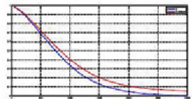
Graphs of probability density function fs(t) and mixture probability density function fmixture
s (t) of the series system with two components are shown in Figure 3a. Graphs of reliability function Rs(t) and mixture reliability function Rmixture
s (t) of the series system with two components are shown in Figure 3b. Graphs of hazard function hs(t) and mixture hazard function hmixtures (t) of the series system with two components are shown in Figure 3c.
Figure 3
2.2. Case 2: A Parallel System of Two Components
For Case 2, the reliability block diagram of a parallel system with two com-ponents is shown in Figure 1b. The reliability function Rs(t) for the parallel system with two components is defined by
(15) Rs(t) = RC(t) + RD(t) − RC(t) RD(t) , t > 0
where RC(t) and RD(t) are the reliability functions of the components C and D respectively. The probability density function fs(t) for the parallel system with two components can be obtained from the equation in (5) as
(16) fs(t) = (1 − RD(t)) fC(t) + (1 − RC(t)) fD(t) , t > 0
where fC(t) and fD(t) are the probability density functions of the components C and D respectively. The hazard function hs(t) for the parallel system with two components can be obtained from the equation in (7) as
(17) hs(t) = (1 − RD
(t)) fC(t) + (1 − RC(t)) fD(t) RC(t) + RD(t) − RC(t) RD(t)
Let’s generate 100 data from Weibull (t;8000,10) distribution for component C in reliability block diagram of parallel system in Figure 1b. Let’s denote the elements of this data set as tC1, tC2, . . . , tC100. Let’s generate 100 data
from Weibull (t;5000,4) distribution for component D in reliability block dia-gram of parallel system in Figure 1b. Let’s denote the elements of this data set as tD1, tD2, . . . , tD100. Let’s take tk = max (tCk, tDk) for k = 1, 2, . . . , 100.
Let’s denote the number of counts tk from component C as nC and from com-ponent D as nD. Thus, we have nC + nD = 100 for generated 100 data from Weibull (t;8000,10) distribution for component C and Weibull (t;5000,4) distribution for component D. Let’s repeat this process 10000 times. So we have nC1, nC2, . . . , nC10000 and nD1, nD2, . . . , nD10000. Let’s define ¯nC =
1 10000 P10000 l=1 nCl and ¯nD = 1 10000 P10000
l=1 nDl. Here 10000 denotes the number
of repetition. Then ˆpC and ˆpD estimates of pC and pD are
(18) pˆC= ¯ nC 100 and ˆpD= ¯ nD 100
where 100 denotes the number of generated data. The mixture reliability func-tion Rmixture
s (t) for the parallel system with two components is defined by (19) Rmixtures (t) = pCRC(t) + pDRD(t), t > 0
where pCand pDare mixing proportions or weighting factors for the components C and D respectively. The mixture probability density function fmixture
s (t) for the parallel system with two components is defined by
(20) fsmixture(t) = pCfC(t) + pDfD(t), t > 0 The mixture hazard function hmixture
s (t) for the parallel system with two com-ponents is defined by (21) hmixtures (t) = f mixture s (t) Rmixture s (t) , t > 0 where fmixture
s (t) and Rmixtures (t) are the mixture probability density function and the mixture reliability function for the parallel system with two components C and D respectively. hmixture
s (t) can be expressed as (22) hmixtures (t) = wC(t)hC(t) + wD(t)hD(t)
in terms of non-constant weights wC(t) and wD(t) and component hazard func-tions hC(t) and hD(t). Where non-constant weights wC(t) and wD(t) are written as (23) wC(t) = pCRC(t) pCRC(t) + pDRD(t) and wD(t) = pDRD(t) pCRC(t) + pDRD(t) where 0 < wC(t) < 1, 0 < wD(t) < 1 and wC(t) + wD(t) = 1. wC(t) and wD(t) are non-constant weights. They change depending on time.
Mixing proportions or weighting factors obtained as ˆpC = 0.9737 and ˆpD = 0.0263 for components C and D of the parallel system with two components respectively using the equations in (18). Graphs of mixture probability density function fmixture
s (t) and its component probability density functions fC(t) and fD(t) for the parallel system with two components are shown in Figure 4a. Graphs of mixture reliability function Rmixture
s (t) and its component reliability functions RC(t) and RD(t) for the parallel system with two components are shown in Figure 4b. Graphs of mixture hazard function hmixture
s (t) and its component hazard functions hC(t) and hD(t) for the parallel system with two components are shown in Figure 4c.
Figure 4
Graphs of probability density function fs(t) and mixture probability density function fmixture
s (t) of the parallel system with two components are shown in Figure 5a. Graphs of reliability function Rs(t) and mixture reliability function Rmixture
s (t) of the parallel system with two components are shown in Figure 5b. Graphs of hazard function hs(t) and mixture hazard function hmixtures (t) of the parallel system with two components are shown in Figure 5c.
Figure 5
2.3. Case 3: A Complex System of Series and Parallel Sub-System For Case 3, the reliability block diagram of a complex system consists of two system. First system is with two components in series. Second sub-system is with two components in parallel. The reliability block diagram of the complex system for case 3 is shown in Figure 1c. The reliability function Rs(t) for the complex system with two sub-systems: two components in series and two components in parallel is defined by
(24) Rs(t) = RE(t) RF(t) RG(t) + RE(t) RF(t) RH(t) −RE(t) RF(t) RG(t) RH(t) , t > 0
where RE(t) and RF(t) are the reliability functions of the components E and F respectively in the series sub-system. RG(t) and RH(t) are the reliability func-tions of the components G and H respectively in the parallel sub-system. The probability density function fs(t) for the complex system with two sub-systems: two components in series and two components in parallel can be obtained from the equation in (5) as (25) fs(t) = fE(t) RF(t) RG(t) +fF(t) RE(t) RG(t) +fG(t) RE(t) RF(t) +fE(t) RF(t) RH(t) + fF(t) RE(t) RH(t) + fH(t) RE(t) RF(t) −fE(t) RF(t) RG(t) RH(t) − fF(t) RE(t) RG(t) RH(t) −fG(t) RE(t) RF(t) RH(t) − fH(t) RE(t) RF(t) RG(t) , t > 0 where fE(t) and fF(t) are the probability density functions of the components E and F respectively in the series sub-system. fG(t) and fH(t) are the probability
density functions of the components G and H respectively in the parallel sub-system.
The hazard function hs(t) for the complex system with two sub-systems: two components in series and two components in parallel can be obtained from the equation in (7) as
(26) hs(t) =
fs(t) Rs(t)
, t > 0
Let’s generate 100 data from Weibull (t;1000,1.5) distribution for component E in reliability block diagram of complex system in Figure 1c. Let’s denote the elements of this data set as tE1, tE2, . . . , tE100. Let’s generate 100 data from
Weibull (t;10000,1.5) distribution for component F in reliability block diagram of complex system in Figure 1c. Let’s denote the elements of this data set as tF1, tF2, . . . , tF100. Let’s generate 100 data from Weibull (t;1000,3) distribution
for component G in reliability block diagram of complex system in Figure 1c. Let’s denote the elements of this data set as tG1, tG2, . . . , tG100. Let’s generate
100 data from Weibull (t;5000,1.5) distribution for component H in reliability block diagram of complex system in Figure 1c. Let’s denote the elements of this data set as tH1, tH2, . . . , tH100. Let’s take tk = min (tEk, tFk, max (tGk, tHk)) for
k = 1, 2, . . . , 100. Let’s denote the number of counts tk from component E as nE, component F as nF, component G as nG and from component H as nH. Thus, we have nE+ nF + nG+ nH= 100 for generated 100 data from Weibull (t;1000,1.5) distribution for component E, Weibull (t;10000,1.5) distribution for component F , Weibull (t;1000,3) distribution for component G and Weibull (t;5000,1.5) distribution for component H. Let’s repeat this process 10000 times. So we have nE1, nE2, . . . , nE10000, nF1, nF2, . . . , nF10000, nG1, nG2, . . . , nG10000 and nH1, nH2, . . . , nH10000. Let’s define, ¯nE= 1 10000 P10000 l=1 nEl, ¯nF = 1 10000 P10000 l=1 nFl, ¯ nG = 100001 P10000 l=1 nGl and ¯nH = 1 10000 P10000
l=1 nHl. Here 10000 denotes the
number of repetition. Then ˆpE, ˆpF, ˆpGand ˆpH estimates of pE, pF, pG and pH are (27) pˆE= ¯ nE 100, ˆpF = ¯ nF 100, ˆpG= ¯ nG 100 and ˆpH = ¯ nH 100
where 100 denotes the number of generated data. The mixture reliability func-tion Rmixture
s (t) for the complex system with two sub-systems: two components in series and two components in parallel is defined by
(28) Rmixtures (t) = pERE(t) + pFRF(t) + pGRG(t) + pHRH(t), t > 0 where pEand pFare mixing proportions or weighting factors for the components E and F respectively in the series sub-system. pGand pHare mixing proportions or weighting factors for the components G and H respectively in the parallel sub-system. The mixture probability density function fmixture
s (t) for the complex system with two sub-systems: two components in series and two components in parallel is defined by
(29) fmixture
The mixture hazard function hmixtures (t) for the complex system with two sub-systems: two components in series and two components in parallel is defined by (30) hmixtures (t) = f mixture s (t) Rmixture s (t) , t > 0 where fmixture
s (t) and Rmixtures (t) are the mixture probability density function and the mixture reliability function for the complex system with two sub-systems: two components in series and two components in parallel respectively. hmixture
s (t) can be expressed as
(31) hmixtures (t) = wE(t)hE(t) + wF(t) hF(t) + wG(t)hG(t) + wH(t)hH(t) in terms of non-constant weights wE(t), wF(t), wG(t) and wH(t), and component hazard functions hE(t), hF(t), hG(t) and hH(t). Where non-constant weights wE(t), wF(t), wG(t) and wH(t) are written as
(32) wE(t) = pERE(t) pERE(t) + pFRF(t) + pGRG(t) + pHRH(t) wF(t) = pFRF(t) pERE(t) + pFRF(t) + pGRG(t) + pHRH(t) wG(t) = pGRG(t) pERE(t) + pFRF(t) + pGRG(t) + pHRH(t) and wH(t) = pHRH(t) pERE(t) + pFRF(t) + pGRG(t) + pHRH(t) Where 0 < wE(t), wF(t), wG(t), wH(t) < 1, and wE(t)+wF(t)+wG(t)+wH(t) = 1. wE(t), wF(t), wG(t) and wH(t) are non-constant weights. They change depending on time. Mixing proportions or weighting factors obtained as ˆpE = 0.9113, ˆpF = 0.0286, ˆpG = 0.0265 and ˆpH = 0.0336 for components E, F , G and H of the complex system with four components respectively using then equations in (27). Graphs of mixture probability density function fsmixture(t) and its component probability density functions fE(t), fF(t), fG(t) and fH(t) for the complex system with four components are shown in Figure 6a. Graphs of mixture reliability function Rmixture
s (t) and its component reliability functions RE(t), RF(t), RG(t) and RH(t) for the complex system with four components are shown in Figure 6b. Graphs of mixture hazard function hmixture
s (t) and its component hazard functions hE(t), hF(t), hG(t) and hH(t) for the complex system with four components are shown in Figure 6c.
Figure 6
Graphs of probability density function fs(t) and mixture probability density function fmixture
s (t) of the complex system with four components are shown in Figure 7a. Graphs of reliability function Rs(t) and mixture reliability function Rmixture
s (t) of the complex system with four components are shown in Figure 7b. Graphs of hazard function hs(t) and mixture hazard function hmixtures (t) of the complex system with four components are shown in Figure 7c.
Figure 7 3. Conclusions
In this study, the mixture reliability functions, mixture probability density func-tions and mixture hazard funcfunc-tions were established for reliability block dia-grams of series, parallel and complex systems. The mixture reliability function, the mixture probability density function and the mixture hazard function, estab-lished for the systems studied, were proposed as an approximation to reliability function, probability density function and hazard function respectively. By the mixture distribution model approximation to system reliability: the function representations were simplified, the function calculations were decreased and the information extracted from the system and its components were increased for reliability block diagrams of series, parallel and complex systems. For instance, the mixture reliability function given in equation (28), the mixture probability density function given in equation (29) and the mixture hazard function given in equation (31) are more simple than reliability function given in equation (24), probability density function given in equation (25) and hazard function given in equation (26). This situation also makes calculations easier. If the number of components in the reliability block diagram increases then the efficiency of mixture distribution model approximation also increases.
The mixture reliability functions obtained from the systems studied are com-pared with the reliability functions obtained from the systems studied: The mixture reliability function created for the series system of two components is a good approximation for the reliability function created for the series system
of two components as seen in Figure 3b. The mixture reliability function cre-ated for the parallel system of two components is a good approximation for the reliability function created for the parallel system of two components as seen in Figure 5b. The mixture reliability function created for complex system that consist of one series and one parallel sub-system is a good approximation for the reliability function created for the complex system that consist of one series and one parallel sub-system as seen in Figure 7b. Also there is no significant difference between the reliability functions and the mixture reliability functions. The mixture probability density functions obtained from the systems studied are compared with the probability density functions obtained from the systems studied: The mixture probability density function created for the series system of two components is a good approximation for the probability density function created for the series system of two components as seen in Figure3a. The mixture probability density function created for the parallel system of two components is a good approximation for the probability density function created for the parallel system of two components as seen in Figure 5a. The mixture probability density function created for complex system that consist of one series and one parallel sub-system is a good approximation for the probability density function created for the complex system that consist of one series and one parallel sub-system as seen in Figure 7a. Also there is no significant difference between the probability density functions and the mixture probability density functions.
The mixture hazard functions obtained from the systems studied are compared with the hazard functions obtained from the systems studied: The mixture hazard function created for the series system of two components can be used as an approximation to the hazard function created for the series system of two components until approximately around 1600 as seen in Figure 3c. If the corresponding component of the system is renewed, the risk decrease with time. So, mixture hazard function is preferable. If the components of the system is not renewed, the risk increase with time. So, hazard function is preferable [7]. Similar ideas can be said for the complex system that consist of one series and one parallel sub-system as seen in Figure 7c. The mixture hazard function created for the parallel system of two components is a good approximation for the hazard function created for the parallel system of two components as seen in Figure 5c. Also there is no significant difference between the hazard function for the parallel system of two components and the mixture hazard function for the parallel system of two components.
It was shown that the system reliability functions, the system probability den-sity functions and the system hazard functions can be expressed in terms of component reliability functions, component probability density functions and component hazard functions respectively using the mixture distribution func-tions. These can be seen in Figure 2, Figure 4 and Figure 6.
The mixture proportions or weighting factors of the components in the mixture distribution model were estimated using the equations in (8), (18) and (27) for the series, parallel and complex systems respectively. The mixture proportions or weighting factors for mixture reliability functions and mixture probability density functions are constants with respect to time. But the mixture propor-tions or weighting factors for mixture hazard funcpropor-tions are not constant and they are functions of time or they change with respect to time as in equations (13), (23) and (32) for the series, parallel and complex systems respectively. The systems examined in this study are prototype systems. So the distribu-tions of the components in the systems and the parameters of the components are assumed to be known. Therefore, parameter estimation of the components have not discussed in this study. In another study, using data from an actual system should determine the distributions of the components, estimate the pa-rameters of the distributions of the components and the weighting factors of the components in the mixture distribution model approximation.
References
1. Andrews, J.D. and Moss, T.R. (2002): Reliability and Risk Assessment, Second Edition, Professional Engineering Publishing Limited: London and Bury St Edmunds, UK. 540s.
2. Bentley, J.P. (1993): An introduction to Reliability and Quality Engineering, Log-man Scientific and Technical, John Wiley & Sons, Inc. New York.
3. Bucar, T., Nagode, M. and Fajdiga, M. (2004): Reliability approximation using finite Weibull mixture distributions, Reliability Engineering and System Safety, 84, 241—251.
4. Campioni, L. and Vestrucci, P. (2006): On system failure probability density func-tion, Reliability Engineering and System Safety, Volume 92, Issue 10, Pages 1321-1327. 5. Elsayed, E.A. (1996): Reliability Engineering, Addison Wesley Longman, Inc. 6. Hahn, G.J. and Shapiro, S.S. (1967): Statistical Models in Engineering, John Wiley & Sons, Inc. New York, Chichester, Brisbane, Toronto.
7. Jiang, R. and Murthy, D.N.P. (1997): Two Sectional Models involving three Weibull Distributions, Quality And Reliability Engineering International, Vol. 13, 83-96. 8. Johnson, N.L., Kotz, S. and Balakrishnan, N. (1994): Continuous Univariate Dis-tributions, Volume1: Second Edition, Wiley Series in Probability and Mathematical Statistics, A Wiley — Interscience Publication: John Wiley & Sons, Inc. New York, Chichester, Brisbane, Toronto, Singapore.
9. Mclachlan, G. and Peel, D. (2000): Finite Mixture Models, Wiley Series in Proba-bility and Statistics Applied ProbaProba-bility and Statistics Section, A Wiley — Interscience Publication: John Wiley & Sons, Inc. New York, Chichester, Weinheim, Brisbane, Singapore, Toronto.
10. Meeker, W. Q. and Escobar, L. A. (1998): Statistical Methods for Reliability Data, John Wiley & Sons Inc. New York.
11. Mettas, A. and Savva, M. (2001): System Reliability Analysis: The Advantages of Using Analytical Methods to Analyze Non-Repairable Systems, IEEE 2001
Proceed-ings Annual Reliability And Maintainability Symposium, Philadelphia, Pennsylvania, USA, January 22-25.
12. Moss, T.R. (2005): The Reliability Data Handbook, Professional Engineering Publishing Limited: London and Bury St Edmunds, UK. 287s.