Benchmarking data mining techniques for segmenting diabetes patients

(1)

T.C.

BAHÇEŞEHİR ÜNİVERSİTESİ

BENCHMARKING DATA MINING TECHNIQUES FOR SEGMENTING

DIABETES PATIENTS

Master Thesis

İnayet ADALI

(2)

T.C

BAHÇEŞEHİR ÜNİVERSİTESİ

INSTITUTE OF SCIENCES

COMPUTER ENGINEERING

BENCHMARKING DATA MINING TECHNIQUES FOR SEGMENTING

DIABETES PATIENTS

Master Thesis

İnayet ADALI

Supervisor: ASSOC.PROF.DR. ADEM KARAHOCA

(3)

T.C. BAHÇEŞEHİR ÜNİVERSİTESİ INSTITUTE OF SCIENCES COMPUTER ENGINEERING

Name of the thesis: BENCHMARKING DATA MINING TECHNIQUES FOR SEGMENTING DIABETES PATIENTS

Name/Last Name of the Student: İnayet ADALI Date of Thesis Defense: Jun .12. 2009

The thesis has been approved by the Institute of Sciences.

Prof. Dr. Bülent ÖZGÜLER Principal of Institute of Sciences ___________________

I certify that this thesis meets all the requirements as a thesis for the degree of Master of Science.

Prof. Dr. Bülent ÖZGÜLER Program Coordinator

___________________

This is to certify that we have read this thesis and that we find it fully adequate in scope, quality and content, as a thesis for the degree of Master of Science.

Examining Committee Members Signature

Assoc.Prof.Dr. Adem KARAHOCA ___________________ Prof.Dr. Nizamettin AYDIN ___________________

(4)

ACKNOWLEDGEMENTS

I would like to express my gratitude to Assoc. Prof. Dr. Adem Karahoca, for not only being such a great supervisor but also encouraging and challenging me throughout my academic program.

I also wish to thank to my mother Engin ADALI, my father Ziver ADALI and İren AĞAN for their mental helps on finishing this thesis. Lastly I want to thank to my grandfather Sabahattin ADALI for his helps on me to maintain in Bahçeşehir University.

(5)

ABSTRACT

BENCHMARKING DATA MINING TECHNIQUES FOR

SEGMENTING DIABETES PATIENTS

İnayet ADALI

M.S. Department of Computer Engineering Supervisor: Assoc. Prof.

Dr. Adem Karahoca

June 2009, 45 pages

Medical researches and questionnaires declare that there are approximately 5 million diabetic patients in Turkey. Unfortunately majority of them don’t realize that they are in danger of diabetes. It is thought difficult to visit a doctor and examine the results of their insulin measurement. I intend to make a benchmarking on data mining techniques for segmenting diabetes patients, which will help on examining the medical results of potential patients. I intend to use datas from İstanbul Diabetes Hospital. It’s needed to benchmark of data mining techniques using socio-demographic data of diabetic patients, in order to reveal diabetes map of Turkey, to find association rules among the social-demographic data and to apply Adaptive Neuro Fuzzy Inference System (ANFIS), multinomial logistic regression (MLR), Bayesian network and rough set. Via benchmarking these used methods, it’s seen that ANFIS is more effective than other methods using diabetes data.

Key words: expert system, Prolog Server Pages (PSP), diabetes diagnosis, WEKA, data mining, adaptive neuro fuzzy inference system (ANFIS), logistic regression

(6)

ÖZET

DİYABET HASTALARININ VERİLERİ KULLANILARAK VERİ MADENCİLİĞİ TEKNİKLERİNİN KARŞILAŞTIRILMASI

İnayet ADALI

Yüksek Lisans, Bilgisayar Mühendisliği Bölümü Tez Yöneticisi: Doç. Dr. Adem

Karahoca

Haziran 2009, 45 sayfa

Tıbbi araştırmalar ve anketler, Türkiye’de 5 milyondan fazla diyabet (şeker) hastası bulunduğunu ortaya koymaktadır. Ancak bu hastalann büyük çoğunluğu maalesef diyabet tehlikesinde olduklannın farkında değildirler. Uzman bir doktoru ziyaret etmek, muayene olmak ve insülin tedavisinde dozajı ayarlamak için doktorla görüşmek hastalara zor gelmektedir. Hem potansiyel hastalann risk oranını belirlemek, hem de diyabetlilerin tedavileri boyunca yol gösterici bir uzman sistem geliştirmek için veri madenciliği tekniklerinin karşılaştinlması istendi. Bu nedenle, İstanbul Diabet Hastenesi verileri kullanıldı. Diyabet hastalannın sosyo-demografik verilerini kullanarak veri madenciliği tekniklerinin karşılaştinlması istendi. Bu amaçla, diyabet hastalannın sahip olduğu veriler ANFIS, multinominal lojistik regresyon, bayes ağı yardımı ve rough set kullanılarak kestirimler yapıldı. Son olarak kıyaslamalar yapıldı ve sonuc olarak, ANFIS’ in daha etkili bir öğrenme ve kestirim aracı olduğu görüldü. Anahtar Kelimeler: uzman sistem, Prolog Server Pages (PSP), diyabet tanı ve tedavisi, WEKA, veri madenciliği, ANFIS, benchmarking, lojistik regresyon.

(7)

TABLES

Table 2.1 : Some variables and descriptions of dataset ... 11

Table 2.2 : Discretization ... 12

Table 2.3 Table of the attributes in Rosetta ... 13

Table 2.4 : List of some Data Mining methods ... 14

Table 2.5 : An information system ... 20

Table 2.6 : Discernibility matrix ... 20

Table 2.7 : Equivalence classes... 21

Table 2.8 : A decision system ... 23

Table 3.1 : Facts on Experiment data set ... 39

Table 3.2 : Rosetta confusion matrix... 40

Table 3.3 : Strength and normalized weight for the classes ... 41

(10)

FIGURES

Figure 2.1 : A Bayesian Network example ... 14

Figure 2.2 : The B-upper and B-lower approximations of X... 21

Figure 2.3 : ANFIS architecture ... 31

Figure 3.1 : Linear Regression Model ... 36

Figure 3.2 : Bayes network classifier ... 37

Figure 3.3 : Best-first decision tree ... 38

Figure 3.4 : Rosetta work screen ... 40

Figure 3.5 : Error Percentages ... 42

(11)

ABBREVIATIONS

AI Artificial Intelligence

ANFIS Adaptive Neuro Fuzzy Inference System BMI Body Mass Index

HDL High Density Lipoprotein LDL Low Density Lipoprotein

MLR Multinomial Logistic Regression PHP Personal Home Pages

PSP Prolog Server Pages

RDBMS Rational Database Management System ROC Receiver Operating Characteristic

(12)

1. INTRODUCTION

Medical researches and questionnaires declare that there are approximately 5 million diabetic patients in Turkey. But unfortunately most of diabetic patients either don’t visit physician regularly or don’t know he is already diabetic. My starting point is to benchmark data mining techniques for segmenting these diabetic patients.

I would like to help diabetic patients or the people who suspect if they have diabetes risk by benchmarking these techniques. I think this segmentation will help patients and physicians during medical treatment for dosage planning stage as well.

The thesis contains 4 main sections. In the first section after introducing the problem diabetes will be explained briefly than the stages of benchmarking will be seen. In addition to this, the 3rd party solutions that work integrated to the diabetes data mining are shortly mentioned about.

The methodologies and materials of thesis are exhibited in section 2. Both functionality and usage are defined in the section supported with formulas and graphics.

The third section has experiments on Weka, Matlab and Rosetta. Bench markings are executed in the section in order to examine performances of data mining techniques and statistical methods.

In the final section, the results that we have reached, and the conclusions that the thesis has given us are shared.

(13)

1.1 Problem Definition

Life is difficult to diabetic patients. They must measure their glucose rate, inject insulin regularly, visit physician and examine the results. After the data measured, by using which technique we can make more time for detecting glucose level. After that Insulin dosage may be planned effectively.

Once data mining is finished, I saw that some of the techniques were not giving me the quite similar results, but by using some techniques I may have better results. Then why should people use worse techniques for segmenting diabetes patients.

Another problem that must be solved by segmentation diabetes data is the diabetic map of Turkey. It’s needed to work on data mining with a knowledge based of diabetic patients. However the knowledge base must be pre-processed before applying data mining techniques. The diabetes segmentation should solve the pre-processing problem and apply data mining techniques such as classification and apply Neuro-Fuzzy Inference System like ANFIS (Adaptive Neuro-Fuzzy Inference System) (Polat & Gunes 2006).

1.2 What is Diabetes?

Diabetes is a disorder of metabolism—the way the body uses digested food for growth and energy. Most of the food people eat is broken down into glucose, the form of sugar in the blood. Glucose is the main source of fuel for the body.

After digestion, glucose passes into the bloodstream, where it is used by cells for growth and energy. For glucose to get into cells, insulin must be present. Insulin is a hormone produced by the pancreas, a large gland behind the stomach.

When people eat, the pancreas automatically produces the right amount of insulin to move glucose from blood into the cells. In people with diabetes, however, the pancreas either produces little or no insulin, or the cells do not respond appropriately to the insulin that is produced. Glucose builds up in the blood, overflows into the urine, and

(14)

passes out of the body in the urine. Thus, the body loses its main source of fuel even though the blood contains large amounts of glucose.

1.2.1 What are the types of diabetes?

The three main types of diabetes are  type 1 diabetes

 type 2 diabetes  gestational diabetes

1.2.1.1 Type 1 Diabetes:

Type 1 diabetes is an autoimmune disease. An autoimmune disease results when the body’s system for fighting infection—the immune system—turns against a part of the body. In diabetes, the immune system attacks and destroys the insulin-producing beta cells in the pancreas. The pancreas then produces little or no insulin. A person who has type 1 diabetes must take insulin daily to live.

At present, scientists do not know exactly what causes the body’s immune system to attack the beta cells, but they believe that autoimmune, genetic, and environmental factors, possibly viruses, are involved. Type 1 diabetes accounts for about 5 to 10 percent of diagnosed diabetes in Turkey. It develops most often in children and young adults but can appear at any age.

Symptoms of type 1 diabetes usually develop over a short period, although beta cell destruction can begin years earlier. Symptoms may include increased thirst and urination, constant hunger, weight loss, blurred vision, and extreme fatigue. If not diagnosed and treated with insulin, a person with type 1 diabetes can lapse into a life-threatening diabetic coma, also known as diabetic ketoacidosis (http://www.hastane.com.tr-translation).

(15)

1.2.1.2 Type 2 Diabetes:

The most common form of diabetes is type 2 diabetes. About 90 to 95 percent of people with diabetes have type 2. This form of diabetes is most often associated with older age, obesity, family history of diabetes, previous history of gestational diabetes, physical inactivity, and certain ethnicities. About 80 percent of people with type 2 diabetes are overweight.

Type 2 diabetes is increasingly being diagnosed in children and adolescents, especially among African American, Mexican American, and Pacific Islander youth.

When type 2 diabetes is diagnosed, the pancreas is usually producing enough insulin, but for unknown reasons the body cannot use the insulin effectively, a condition called insulin resistance. After several years, insulin production decreases. The result is the same as for type 1 diabetes—glucose builds up in the blood and the body cannot make efficient use of its main source of fuel.

The symptoms of type 2 diabetes develop gradually. Their onset is not as sudden as in type 1 diabetes. Symptoms may include fatigue, frequent urination, increased thirst and hunger, weight loss, blurred vision, and slow healing of wounds or sores. Some people have no symptoms (http://www.hastane.com.tr-translation).

1.2.1.3 Gestational Diabetes

Some women develop gestational diabetes late in pregnancy. Although this form of diabetes usually disappears after the birth of the baby, women who have had gestational diabetes have a 40 to 60 percent chance of developing type 2 diabetes within 5 to 10 years. Maintaining a reasonable body weight and being physically active may help prevent development of type 2 diabetes.

About 3 to 8 percent of pregnant women in Turkey develop gestational diabetes. As with type 2 diabetes, gestational diabetes occurs more often in some ethnic groups and among women with a family history of diabetes. Gestational diabetes is caused by the

(16)

hormones of pregnancy or a shortage of insulin. Women with gestational diabetes may not experience any symptoms (Swapnil N. Rajpathak, 2008).

1.2.2 Diabetes in Youth

The SEARCH for Diabetes in Youth multicenter study, funded by the Centers for Disease Control and Prevention and the National Institutes of Health, has determined that (Polat & Gunes, July 2009);

 based on data from 2002 to 2003, a total of 8,000 youth in Turkey were newly diagnosed with type 1 diabetes each year. In addition, about 1,700 youth were newly diagnosed with type 2 diabetes each year.

 non-Hispanic white youth had the highest rate of new cases of type 1 diabetes.  type 2 diabetes was rarely diagnosed among youth younger than 10 years of age.

1.2.3 Other Types of Diabetes

A number of other types of diabetes exist. A person may exhibit characteristics of more than one type. For example, in latent autoimmune diabetes in adults (LADA), also called type 1.5 diabetes or double diabetes, people show signs of both type 1 and type 2 diabetes(T.Zhang - S. Pan, 2009).

Other types of diabetes include those caused by

 genetic defects of the beta cell—the part of the pancreas that makes insulin—such as maturity-onset diabetes of the young (MODY) or neonatal diabetes mellitus (NDM)  genetic defects in insulin action, resulting in the body’s inability to control blood

glucose levels, as seen in leprechaunism and the Rabson-Mendenhall syndrome  diseases of the pancreas or conditions that damage the pancreas, such as pancreatitis

and cystic fibrosis

 excess amounts of certain hormones resulting from some medical conditions—such as cortisol in Cushing’s syndrome—that work against the action of insulin

(17)

 medications that reduce insulin action, such as glucocorticoids, or chemicals that destroy beta cells

 infections, such as congenital rubella and cytomegalovirus

 rare immune-mediated disorders, such as stiff-man syndrome, an autoimmune disease of the central nervous system

 genetic syndromes associated with diabetes, such as Down syndrome and Prader-Willi syndrome

1.2.4 How is diabetes diagnosed?

The fasting blood glucose test is the preferred test for diagnosing diabetes in children and nonpregnant adults. The test is most reliable when done in the morning. However, a diagnosis of diabetes can be made based on any of the following test results, confirmed by retesting on a different day:

 A blood glucose level of 126 milli grams per deciliter (mg/dL) or higher after an 8-hour fast. This test is called the fasting blood glucose test.

 A blood glucose level of 200 mg/dL or higher 2 hours after drinking a beverage containing 75 grams of glucose dissolved in water. This test is called the oral glucose tolerance test (OGTT).

 A random—taken at any time of day—blood glucose level of 200 mg/dL or higher, along with the presence of diabetes symptoms.

Gestational diabetes is diagnosed based on blood glucose levels measured during the OGTT. Glucose levels are normally lower during pregnancy, so the cutoff levels for diagnosis of diabetes in pregnancy are lower. Blood glucose levels are measured before a woman drinks a beverage containing glucose. Then levels are checked 1, 2, and 3 hours afterward. If a woman has two blood glucose levels meeting or exceeding any of the following numbers, she has gestational diabetes: a fasting blood glucose level of 95 mg/dL, a 1-hour level of 180 mg/dL, a 2-hour level of 155 mg/dL, or a 3-hour level of 140 mg/dL. (Notes from the doctor of İstanbul Diabet Hospital. Dr. Huriye Alasya)

(18)

1.3 Related Works

Any researcher could find Data mining articles on diabetes, when he searches about data mining on Internet or scientific libraries. Some related works about diabetes and data mining are found in the literature research, and mentioned about them in the following section. When we investigated them, we saw they usually do 2 different methods also none of them make benchmarking between the methods they used so none of the works fits the problems defined in the Section 1.1.

There is non-ignorable number of people who suffer from diabetes. And, most of them are not aware that they have diabetes. Predictability of diabetes plays an important role for the patient’s early treatment process. However, the correct prediction percentage of current algorithms is low. A new approach, called Homogeneity-Based Algorithm (HBA), is applied together with traditional classification approaches to enhance the accuracy of diabetes prediction. In contrast to traditional approaches, this new approach proposes a new method to optimally control the over fitting and overgeneralization behaviors of classification on this dataset. Some computational results seem to indicate that the proposed approach significantly performs better than current approaches. Over fitting and overgeneralization behaviors of current classification algorithms cause low accuracies in processing the dataset. The obtained results in relation with HBA appear to be very important both for accurately predicting diabetes and also for the data mining community, in general. (H.Nguyen and A.Pham 2007)

In this study, they get better result when compared to MLR. We will try to get better results from diabet data by using different methods and benchmarked the methods used.

Pima Indians living in near Phoenix, Arizona, who are usually susceptible to diabetes, were tested in accordance with the criteria of World Health Organization. An analysis of findings of project conducted is expected to be done based on a number of

sources which are available publicly including at

(19)

The analysis may include following:

1. An analysis based on 798 females with eight continuous variables measured for each female.

2. An exploratory statistical analysis performed on the sample dataset.

3. Use of Ripley’s training dataset to construct a logistic model for prediction the variable “type.

4. A formation of classification tree grown for Pima Indians diabetes data based on a training set of size 200.

5. Control of reduction of dimension of the problem by applying the principal components analysis to dataset.

6. Summary of the problem and results of the analysis.

Pima Indians network is a great dataset for segmenting, they used exploratory statistical analysis on this dataset after the analysis they get pretty good results on the dataset. When compared to Pima India dataset our dataset is similar it has less patients but more variables we will try to have better results from Pima India dataset if we can.

Diabetes is a disease in which the body has a difficulty in regulating insulin. This may lead to many diseases such as kidney disease, blindness, nerve damage, blood vessel damage besides contributing to heart disease. The principal component analysis (PCA) and adaptive neuro-fuzzy inference system (ANFIS) have been used as a method to diagnose the diabetes disease. The dataset for analysis was obtained from the sources held by the National Institute of Diabetes and Digestive and Kidney Disease, where all patients are Pima-Indian women at least 21 years old and living in Phoenix, Arizona, USA. To do this, an expert system which works in two stages has been applied. In first stage, the dimension of diabetes database was reduced from 8 to 4 features using PCA. And, in the second, an adaptive neuro-fuzzy inference system (ANFIS) classifier was used to diagnosis of diabetes disease. As a result, it has been found that the use of PCA and ANFIS in combination give a diagnostic and classification accuracy of 89.47%, making it very promising with regard to other classification applications in the literature for this problem. (K. Polat, S. Güneş-2008)

(20)

In this study ANFIS used on diabetic patients. Our approach is to see differences between ANFIS and other methods. We will see if there are any better result can be found.

(21)

2. MATERIALS & METHODS

2.1 Data Set Preparation for diabetics

The dataset that was used in the thesis consist of 24 variables of 470 subjects 277 male and 193 female who were interviewed in a İstanbul Diabet Hospital and also 16 different treatment type. Most of subjects are known as diabetic and all of them are under diabetes treatment. In our work it’s tried to find any relation between diabetes risk and height, weight, gender, HbA%, uric glucose, blood pressure, keton, protein, micros, Mic. Alb, polifaji, poliuri, polidipsi, total cholesterol, side effects such as xerostomia and a ratio that is called frame. The waist/hip ratio (Frame) may be a predictor in diabetes.

Having searched the literature, it’s seen that works were dealing with binary results (1=healthy, 0=diabetic). In this work it’s desired to make a step beyond, and worked on fuzzy dependent variable.

The dependent variable in the dataset is Glucose rate and independent variables are:

i. Height ii. Weight iii. HbA% iv. Uric glucose v. Blood Pressure vi. Keton vii. Protein viii. Mikros ix. Mic.Alb x. Polifaji xi. Poliuri xii. Polidipsi

xiii. Total cholesterol xiv. Gender

(22)

xv. Frame (Waist/Hip ratio) xvi. Side Effects(7 Different) xvii. Medicine(16 Types)

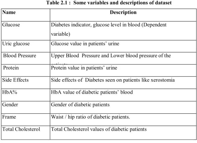
Some variables of the dataset had already fuzzy values, such as frame. However some of them didn’t have fuzzy values such as polidipsi, glucose. Some variables of the dataset used in the thesis are shown in Table 2.1.

Table 2.1 : Some variables and descriptions of dataset

Name Description

Glucose Diabetes indicator, glucose level in blood (Dependent variable)

Uric glucose Glucose value in patients’ urine

Blood Pressure Upper Blood Pressure and Lower blood pressure of the patients

Protein Protein value in patients’ urine

Side Effects Side effects of Diabetes seen on patients like xerostomia HbA% HbA value of diabetic patients’ blood

Gender Gender of diabetic patients

Frame Waist / hip ratio of diabetic patients.

Total Cholesterol Total Cholesterol values of diabetic patients

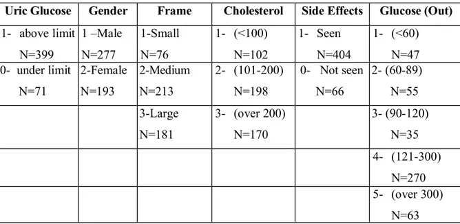
The main purpose of preprocessing data was to make fuzzy the variable in order to use them in ANFIS as a fuzzy inference system. Some variables and their fuzzy values are shown in Table 2.2.

(23)

Table 2.2 : Discretization N=470

Uric Glucose Gender Frame Cholesterol Side Effects Glucose (Out) 1- above limit N=399 1 –Male N=277 1-Small N=76 1- (<100) N=102 1- Seen N=404 1- (<60) N=47 0- under limit N=71 2-Female N=193 2-Medium N=213 2- (101-200) N=198 0- Not seen N=66 2- (60-89) N=55 3-Large N=181 3- (over 200) N=170 3- (90-120) N=35 4- (121-300) N=270 5- (over 300) N=63 Since the purpose is same the other estimation method, and it’s to define a relationship between dependent variable and independent variables by using minimum variables; then it’s needed to decrease the number of inputs to the least meaningful number.

The function exhsrch in MATLAB performs an exhaustive search within the available inputs to select the set of inputs that most influence the diabetes diagnosis. The first parameter to the function specifies the number of input combinations to be tried during the search.

(24)

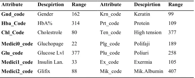
Rosetta data set

Table 2.3: Table of the attributes in Rosetta.

Attribute Descpirtion Range Attribute Descpirtion Range

Gnd_code Gender 162 Krn_code Keratin 99

Hba_Code HbA% 314 Prt_code Protein 109

Chl_Code Cholestrole 80 Ten_code High tension 377 Medici0_code Gluchopage 22 Plg_code Polifaji 189

Glu_code Glucose Lvl 377 Plu_code Poliuri 258

Medici1_code Insulin Lan. 33 Ex_code Exermia 105 Medici2_code Glifix 88 Mik_code Mik.Albumin 407

2.2 Data Mining Methods

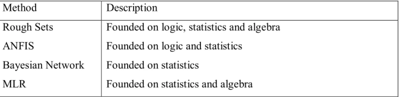
A variety of data mining methods exists. Data mining (sometimes called data or knowledge discovery) is the process of analyzing data from different perspectives and summarizing it into useful information –information that can be used to increase revenue, cuts costs, or both. Data mining software is one of a number of analytical tools for analyzing data. It allows users to analyze data from many different dimensions or angles, categorize it, and summarize the relationships identified. Technically, data mining is the process of finding correlations or patterns among dozens of fields in large relational databases. In our thesis, some data mining methods on social-demographic data of the users were applied. Correction and actuality of the data is very important for data mining for diabetes. We have listed a few methods we have encountered in Table 2.4

(25)

Table 2.4: List of some Data Mining methods. Method Description Rough Sets ANFIS Bayesian Network MLR

Founded on logic, statistics and algebra Founded on logic and statistics

Founded on statistics

Founded on statistics and algebra

Selection of Methods

We have chosen to study the methods Rough Sets, MLR, Bayesian and ANFIS. We chose them because we wanted to study methods which have been used on the diabetic patients data in the literature.

2.2.1 Bayesian Networks

Bayesian, or belief networks, is a method to represent knowledge using directed acyclic graphs (DAG's). The vertices are events which describe the state of some part of the desired universe in some time interval. The edges represent relations between events, and the absence of edges represents independence between events.

A variable takes on values that correspond to events. Variables may be discrete or continuous. A database is denoted D in the following, the set of all variables U, and a Bayesian network-structure is denoted B. If D consists of all variables in U, then D is complete. Two structures are said to be equivalent if they have the same set of probability distributions.

The existing knowledge of an expert or set of experts is encoded into a Bayesian network, then a database is used to update the knowledge, and thus creates one or several new networks.

Bayesian network is illustrated. A disease is dependent on age, work and environment. A symptom is again dependent on a disease.

(26)

Figure 2.1: A Bayesian Network example.

2.2.1.1 Theoretical Overview

In probability theory, P(A) denotes the probability that event A will occur. Belief measures in Bayesian formalism obeys the three basic axioms of probability theory:

 

0P A 1 (2.1)



the prior probability(N Friedman, D Geiger, M Goldszmidt ,1997). WORK

Environment

Age

Disease

(27)

Probability can be seen as a measure of belief in how probable outcomes are, given an event (subjective interpretation). It can also be interpreted as a frequency; how often it has happened in the past (objective interpretation).

2.2.1.2 Applied in Data Mining

When Bayesian Networks are applied in Data Mining, the user may want to apply techniques to learn the structure of a Bayesian network with one or more variables, or to reason on a structure that is already known.

2.2.1.2.1 One Variable

With only one variable, the task is to compute a distribution for the variable given any database. For instance, if we want to compute the probability distribution for a coin that is flipped, the distribution for the variable  would be:



, ,



h

(28)

2.2.1.2.2 Known Structure

If the structure of the network, h S

B , is known in advance, the aim of the analysis is to compute the probabilities on the vertices from the database D. If the database is complete, and the variables are discretized into r different outcomes, the probabilities can be computed according to the following formula:





' 1 ' 1 1 , , i q n ijk ijk h m S i j ij ij N N p C D B N N       



(2.7)

2.2.1.2.3 Learning Structure and Variables

To learn a structure, we want to generate candidate Bayesian Networks, and choose the structure that is best according to the database we have.

The probability distribution in equation gives the probability distribution for the next observation after looking in the database:



1 , ,





1 , ,





,



h S h h h m S m S S B p C  D B  



p C  D B  p B D  (2.8)

To find a Bayesian Network B for a database D, we can use metrics together with a search algorithm. The metrics approximate equation , and some of the metrics are:

 Bayes Factor (BF)  Bayesian Dirichlet (BD)  Maximum a Posteriori (MAP)  A Information Criterion (AIC)  Bayes Information Criterion (BIC)  Minimum Description Length (MDL)

(29)

Some search methods that exist are:

 Local Search - a heuristic search algorithm on the graph.

 Iterated Hill-Climb - uses Local Search, but avoids getting stuck in a local maxima.

If data are missing in the database, it can either be filled in using the posterior distribution. Or we can use Gibbs sampling, which approximates the expectation of any function with respect to it's probability distribution. Another alternative is to use the expectation-maximization (EM)-algorithm which can be used to compute a score from the BIC-metric. (RE Neapolitan – 2003)

2.2.1.3 Properties

Noise: Missing data can be filled in using Gibbs sampling or the posterior distribution. The method is relatively resistant to noise.

Consistency: Bayesian Networks are able to reason with uncertainty. Uncertainty in the data will be included in the model as probabilities of different outcomes.

Prior knowledge: In order to make the Bayesian network structure, it has to be learned from the database. It can also exist as prior knowledge.

Output: The output from Bayesian Network algorithms is a graph, which is easy to interpret for humans.

Complexity: There exist classifiers that perform in linear time, but further iterations give better results.

Retractability: The method is statistically founded, and is always possible to examine why the bayesian method produced certain results.

(30)

2.2.2 Rosetta Rough Sets

The Rough Sets method was designed as a mathematical tool to deal with uncertainty in AI applications. Rough sets have in the last years also proven useful in Data Mining. The method was first introduced by Zdzislaw Pawlak in 1982, the work have been continued by others. This section is a short introduction to the theory of Rough Sets.

2.2.2.1 Theoretical Overview

The starting point of Rough Sets theory is an information system, an ordered pair

A



U A,



. U is a non empty finite set called universe, A is a non empty finite set of attributes. The elements

_

x₁,...,x_n

_

of the universe are called objects, and for each attribute aA, a(x) denotes the value of attribute a for object x U . It is often useful to illustrate an information system in a table, called an information system table. One of the most important concepts in Rough Sets is indiscernibility, denoted IND(). For an information system A



U A,



, an indiscernability relation is:

 







2

 



, :

IND B  x y U a x a y for every aB , (2.10)

Where B A. The interpretation of x IND B x₁

_{ }

₂ is that the objects x and ₁ x can not ₂

be separated by using the attributes in the set B. The indiscernible objects can be classified in equivalence classes:

 

x _B 



y U :



x y,



IND B

 



, (2.11)

again B A.

 

x _B denotes an equivalence class based in the attributes in set B. The set U/IND(B) is the set of all equivalence classes in the relation IND(B). Intuitively the objects of an equivalence class are indiscernible from all other objects in the class, with respect to the attributes in the set B. In most cases we therefore consider the equivalence classes and not the individual objects. The discernibility matrix of an information

(31)



( (



, 1,...,

ij i j

c  aA a x a x for i j n (2.12)

hence, c_{i j}_, contains the attributes upon witch classes x and _i x_j differs (Wieczorkowska, 1999).

Some of the objects attributes may be less important than others when doing the classification. An attribute a is said to be dispersible or superfluous in B A if IND(B)=IND(B-{a}) Otherwise the attribute is indispensable in B. A minimal set of all the attributes that preserves the partitioning of the universe is called a reduct, RED. Thus a reduct is a set of attributes B A such that all attributes aA B are dispensible and IND(B)=IND(A). There are also object-related reducts that gives the set of attributes needed to separate one particular object/class from all the other. The theory is illustrated in the example below.

Table 2.5. An information system object a b c 1 1 2 3 2 1 3 2 3 1 2 3 4 2 1 3 5 2 1 3 6 1 2 3 7 1 3 3

Table 2.6. Discernibility matrix E1 E2 E3 E4 E1  ab bc b E1 ab  abc ab E1 bc abc  c

(32)

Example 1 Consider the small information System A



U A,



, illustrated in Tab??. We see that some of the objects have the same value for all of the attributes, for instance objects 1 and 6, and objects 4 and 5. These objects are indiscernible by attributes a through c, and theses objects are of the same equivalence class. Table 2.5 illustrate the equivalence classes, the attributes and the number of objects from the universe that are indiscernible by attributes a through c. The discernibility matrix for A is shown in Table 2.6, and the reduct for A is, RED A

  

 b c,



(Z Pawlak , 2000).

Table 2.7. Equivalence classes Class a b c

E1 1 2 3 50

E2 2 1 3 11

E3 1 3 2 10

E4 1 3 3 19

The next to define is the lower and upper approximation, Rough definability of sets and the Rough membership function. The lower and upper approximation are used to classify a set of objects, X, from the universe that may belong to different equivalence classes. Let BA and X U, the B-lower, BX and B-upper, BX approximation

are:

 



:



B BX  x U x X (2.13)

 



:



B BX  x U x X  (2.14)

Hence this is a way to approximate X using only the attributes in the set B A. The set BX BX is called the boundary of X. Intuitively, the objects in BX are the objects

that are certain to belong to X, while the objects in BX are possible members of X, as

(33)

Figure 2.2: The B-upper and B-lower approximations of X.

If BX  and BX U then X is said to be Roughly B-definable. If BX  and BX U then X is said to be Internally B-undefinable. If BX  and BX U then X is said to be Externally B-undefinable.

If BX  and BX U then X is said to be Totally B-undefinable

The rough membership function _B



x X,



, where xX , is given by:







 



 

B





, , B , 0 , 1 B B B x X x X x X hence x X x       (2.15)

The rough membership function denotes the frequency of

 

x _B in X, or the probability of X being a member of

 

x _B(L Polkowski, A Skowron – 1998).

A natural extension of the information system is the decision system. A decision system is an information system with an extra set of attributes, called decision attributes, hence A=



U A, D



. In most cases the set D has only one element, D

 

d , and we will use this simplification in the rest of this section. The decision attribute, d, reflects a decision made by an expert. The value of d, V is often a _D

(34)

set of integers {1,...,r(d)}, where r(d) denotes the range of d. It is also possible to represent non numerical decisions, but then it is much simpler to encode the decision into integers, e.g. false and true can be encoded 0 and 1 respectively. The partitioning

 







1  



/ ,..., _{r d}

U IND d  X X of the universe is denoted a decision class, and is a classification of the objects in A determined by the decision attribute d. A decision system is said to be consistent if for all(Z Pawlak , 2002).

 

/ , /

i j i j

E U IND A there excists an X U IND d such that E X (2.16)

Otherwise, the decision system is inconsistent. An inconsistent system is a system where two or more of the objects have the same value for the set of attributes A, hence belonging to the same equivalence class, but the decision attribute d differs. A Decision table is a table of the indiscernability classes, the attributes and the decision attribute. The example below illustrates this.

Table 2.8. A decision system

Class a b c d E1 1 2 2 1 50 E2 2 3 2 2 30 E3 1 2 3 2 10 E4a 2 1 3 2 9 E4b 2 1 3 3 1

Example 2 Consider the decision system A=



U A, ,

 

d



as an extension of the information system in Table 2.6 , illustrate in Table 2.7. We see that there is an inconsistency in class E , where 10 of the objects have decision 2 and one object has ₄

(35)

2.2.2.2 Applied in Data Mining

When using rough sets as a algorithm for data mining, we generate decision rules that map the value of an objects attribute to a decision value. The rules are generated from a test set. If A=



U A, 

 

(36)

identical to the set of definite rules. A threshold value greater than 0.5 maps the value of an objects attributes of an inconsistent equivalence class into only one decision class, where as a threshold value below 0.5 may map into several decision classes (RW Swiniarski, A Skowron , 2003).

Example 4 Assume thresholds for decision system from Table 2.8:

  _tr 1 for E we get no rules₄ .

  _tr 0.6 for E we get one rule E₄ : ₄:a b c_{2 1} 3d₂

  _tr 0.1 for E we get two rules₄ : – I E: ₄:a b c_{2 1} 3d₂

– II E: ₄:a b c_{2 1} 3d₃

Definite and default rules generated directly from the training set, tends to be very specialized. This can be a problem when the rules are applied to unknown data, because many of the objects may fall outside, i.e. not match, of the specialized rules. If we make the rules more general, chances are that a greater number of the objects can be matched by one or more of the rules. One way to do this is to remove some of the attributes in the decision system, and by this glue together equivalence classes. This will certainly increase the inconsistency in the decision system, but by assuming that the attributes removed only discerns a few rare objects from a much larger decision class, this may not be a problem in most cases.

Example 5 Assume we want to classify a new object, with attributes: a b c and _{2 1 2} d . ₂

With the specialized rules from example 1.3 we can not make a match. If we glue together classes E and ₂ E by removing attribute b we get these new rules: ₃

 E a c₁: _{1 3}d₁

 E E₂, ₃:a c_{2 2}d₂

(37)

2.2.2.3 Properties

The subsections below compare the Rough Set method to the criterias outlined in formulas section. This comparison will give us a framework that can be used to compare the various data mining techniques.

Noise: The rough set method is capable of handling most types of noise. If the input data is missing an attribute that is dispencible then the classification process is not affected. If the input data are missing important attributes, then the Rough Sets can not classify the object and the object must be thrown away. There are algorithms implemented that can 'guess' the value of a missing attribute, by doing statistical insertion among others, and thereby keeping the object.

Consistency: As described before, the default rules in Rough Sets can handle inconsistency in the information system quite nicely. In fact, as pointed out, it may be a advantage to introduce inconsistency, by removing attributes, to make the decision rules more general.

Prior Knowledge: Rough set method does not use prior knowledge when generating default rules. As mentioned before the default rules generated by Rough Set algorithms are generated only from the objects in the input data.

Output:The output from the Rough Set algorithms are rules, preferably default rules. These rules can then be uses to predict decisions based on the input attributes. By making variations in the threshold value,  one can tune the number of default rules to _tr

get the most optional result. Rules are easy for humans to interpret and use.

Complexity: The complexity of partitioning is O(nlog(n)), a sort algorithm. Computing the reducts is NP-complete, but there are approximation algorithms (genetic, Johnson, heuristical search) that have proven very efficient.

Retractability: It is easy for the user to find out how the results were generated. This is because Rough Sets method can display the indiscernability classes it created and the

(38)

distribution of the objects in these classes. The user can from this confirm the rules generated, and argument, in basis of the classes, why the rules are correct.

To experiment with the methods chosen, we selected the tools Rosetta, which is a Rough Set analysis tool and AutoClass, which is a Bayesian Networks classifier. The experiments were done on the Diabet Hospital Archives.

The Diabet Hospital Archives: The Diabet Hospital Archive is a large one, which has been developing for more than ten years. It contains data from all over Turkey

Most attributes in the archive are composed differently which for instance describe types of failures. Important information are usually provided. There are several missing attribute values in the archives for some patients.

2.2.2.4 The Tools

2.2.2.4.1 AutoClass - A Bayesian Networks Classifier

AutoClass is a tool for unsupervised classification using Bayesian methods to determine the optimal classes. AutoClass was developed at the NASA Ames Research Center.

In AutoClass, data must be represented in a data vector, with discrete nominal values or real scalar values. Each information vector is called a case, but we will still use the term object for each vector. The vectors can be stored in text- or binary files.

A class is a particular set of attribute (or parameter) values and their associated model. A model is either Single multinomial, Single normal or Multi normal. The first two models assume that attributes are conditionally independent, given a class; the probability that a class would have a particular value of any attribute depend only on the class and is independent of all other attribute values. The Multi normal model expresses mutual dependencies within the class.

(39)

2.2.2.4.2 Rosetta - A Rough Set Toolkit for Analysis of Data

Rosetta is a toolkit for pattern recognition and Data Mining, within the framework of Rough Sets. It is developed as an cooperative effort between the Knowledge System Group at NTNU, Norway and the Logic Group at the University of Warsaw, Poland.

Rosetta runs on every platform, and consists of a kernel and a Graphical User Interface (GUI). The user interacts with the kernel through the GUI, but the kernel is an independent unit. The GUI in Rosetta relies on human interaction and human editing. Data are imported as a decision table from a text file.

The first line contains the attribute names, the second contains the attribute types; integers, real numbers (float) or strings. Then the objects are listed successively. Missing attributes are denoted Undefined.

Rosetta organizes the data in a project and displays relations between the various project items in project trees. Through these trees the user can monitor and manually edit the steps in the process.

Rosetta has also a possibility for testing the rules that have been generated. The rules are applied on a test set with known decision values. The result from the test is a confusion matrix, which is a matrix where the predicted decisions values are compared to the actual decision values. The steps done on the data are recorded together with the data, therefore reproduction of the results are easy to do.

(40)

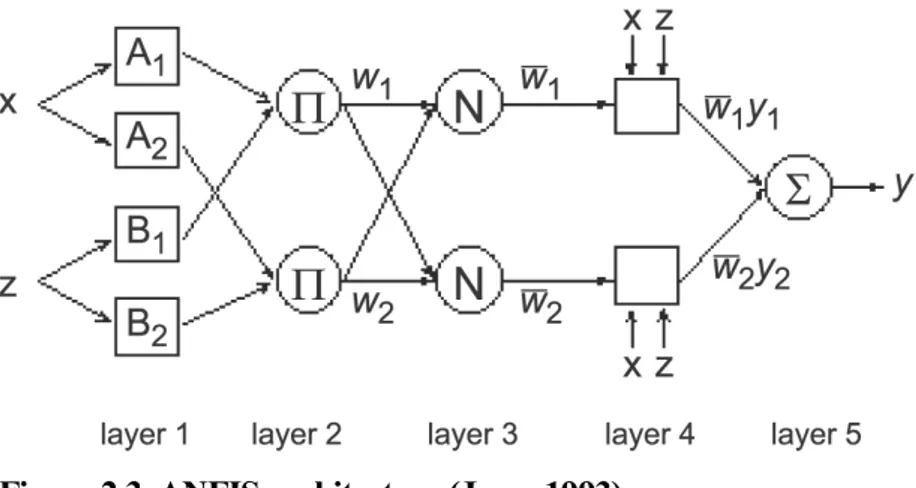
2.2.3 Adaptive Neuro Fuzzy Inference System (ANFIS)

As a neural-fuzzy system, ANFIS is a combination of neural networks and fuzzy systems in such a way that neural networks or neural networks algorithms are used to determine parameters of fuzzy system. This means that the main intention of neural-fuzzy approach is to create or improve a neural-fuzzy system automatically by means of neural network methods. Adaptive neuro fuzzy inference system basically has 5 layer architectures and each of the function is explained in detail below (Sojda 2007; Seising 2006):

Layer 1 Every mode in this layer is an adaptive node with a node function where x (or y) is the input to node I and Ai

_

or Bi₂

_

is a linguistic label and

1

i

O is the membership grade of fuzzy set A



A A B₁, ₂, ₁ or B₂



and it specifies the degree to which the given input x (or y) satisfies the quantifier A. The membership function for A can be parameterized membership function as given in equation 1 or normally known as Bell function and

_

a b c_i, ,_i _i

_

is the parameter set

 











2



1 1 / i Ai x b x ci ai     , (2.19)

 

1 i Ai O  x , i = 1,2,

 

1 2 i Bi O  _ y , i = 3,4, (2.20)

Layer 2 Every node in this layer is a fixed node labeled M, whose output is the product of all the incoming signals each node output represents the firing strength of a rule.

   

2

i i Ai Bi

O   x y , i = 1,2, (2.21)

Layer 3 Every node in this layer is a fixed node labeled N. The ith node calculates the ratio of the ith rule’s firing strength to the sum of all rules’ firing strengths. Outputs of this layer are called normalized

(41)

3 1 2 i i i O        , i = 1,2, (2.22)

Layer 4 Every node I in this layer is an adaptive node with a node function. Where wi is a normalized firing strength from layer 3 and

_

pi qi ri, ,

_

is the parameter set of this node. Parameters in this layer are referred to as consequent parameters.





4

i i i i i i i

O  f  p xq yr , i = 1,2, (2.23)

Layer 5 The single node in this layer is a fixed node labeled , which computes the overall output as the summation of all incoming signals. Overall output:

2 2 4 1 1 1 2 i i i i i i i f O f         



, (2.24)

For simplicity, we assume that the fuzzy inference system under consideration has two input x and y and one output z. For a first-order Sugeno fuzzy model, a common rule set with two fuzzy if-then rules is the following:

Rule 1: If x is A1 and y is B1, the f1 = p1 x + q1 y + r1, Rule 2: If x is A2 and y is B2, the f2 = p2 x + q2 y + r2.

The corresponding equivalent ANFIS architecture is as shown in Figure 4.9, where nodes of the same layer have similar functions. ANFIS has hybrid learning capability which compromised of back propagation and least square method.

(42)

Figure 2.3 ANFIS architecture (Jang, 1993).

2.2.4 Multinomial Logistic Regression

Multinomial logistic regression is used when the dependent variable in question is nominal and consists of more than two categories. In our work, multinomial logistic regression would be appropriate, because we are trying to determine how factors to predict glucose level causing diabetes disease.

The multinomial logistic model assumes that data are case specific; that is, each independent variable has a single value for each case. The multinomial logistic model also assumes that the dependent variable cannot be perfectly predicted from the independent variables for any case.













exp Pr 1 exp i j i J i j j X y j X     

_

(2.25)









1 Pr 0 1 exp i J i j j y X    

_

, (2.26)

According to multinomial logistic regression model, which is defined in (7) and (8), the ith is individual, yi is the observed outcome and Xi is a vector off explanatory variables. The unknown parameters βj are typically estimated by maximum likelihood (Keles & Keles 2006).

(43)

Data mining (sometimes called data or knowledge discovery) is the process of analyzing data from different perspectives and summarizing it into useful information -information that can be used to increase revenue, cuts costs, or both. Data mining software is one of a number of analytical tools for analyzing data. It allows users to analyze data from many different dimensions or angles, categorize it, and summarize the relationships identified. Technically, data mining is the process of finding correlations or patterns among dozens of fields in large relational databases.

In our thesis, some data mining methods on social-demographic data of the users were applied. Correction and actuality of the data is very important for data mining for diabetes.

2.2.5 ANFIS vs. MLR

Artificial Neural Networks (ANNs) and Fuzzy Logic (FL) have been increasingly in use in many engineering fields since their introduction as mathematical aids by McCulloch and Pitts, 1943, and Zadeh, 1965, respectively. Being branches of Artificial Intelligence (AI), both emulate the human way of using past experiences, adapting itself accordingly and generalizing. While the former have the capability of learning by means of parallel connected units, called neurons, which process inputs in accordance with their adaptable weights usually in a recursive manner for approximation; the latter can handle imperfect information through linguistic variables, which are arguments of their corresponding membership functions.

Although the fundamentals of ANNs and FL go back as early as 1940s and 1960s, respectively, significant advancements in applications took place around 1980s. After the introduction of back-propagation algorithm for training multi-layer networks by Rumelhart and McClelland, 1986, ANNs has found many applications in numerous inter-disciplinary areas (Patterson 1994; Rumelhart & McCelland 1986; McCelland & other 1986, pp.216-271). On the other hand, FL made a great advance in the mid 1970s with some successful results of laboratory experiments by Mamdani and Assilian (1975, pp.1-13). In 1985, Takagi and Sugeno (1985, pp.116-132) contributed FL with a new rule-based modeling technique. Operating with linguistic expressions, fuzzy logic can

(44)

use the experiences of a human expert and also compensate for inadequate and uncertain knowledge about the system. On the other hand, ANNs have proven superior learning and generalizing capabilities even on completely unknown systems that can only be described by its input-output characteristics. By combining these features, more versatile and robust models, called “neuro-fuzzy” architectures have been developed (Culliere et al. 1995, pp.2009-2016).

In a control system the plant displaying nonlinearities has to be described accurately in order to design an effective controller. In obtaining the model, the designer has to follow one of two ways. The first one is using the knowledge of physics, chemistry, biology and the other sciences to describe an equation of motion with Newton’s laws, or electric circuits and motors with Ohm’s, Kirchhoff’ s or Lentz’s laws depending on the plant of interest. This is generally referred to as mathematical modeling. The second way requires the experimental data obtained by exciting the plant, and measuring its response. This is called system identification and is preferred in the cases where the plant or process involves extremely complex physical phenomena or exhibits strong nonlinearities.

Conventional control methods rely upon strong mathematical modeling, analysis, and synthesis. In case where mathematical models are available conventional control theory acts as a powerful tool for controlling even complex systems. On the other hand obtaining a mathematical model for a system can be rather complex and time consuming as it often requires some assumptions such as defining an operating point and doing linearization about that point and ignoring some system parameters, etc. This fact has recently led the researchers to exploit the neural and fuzzy techniques in modeling and control of complex systems.

Although fuzzy logic allows one to model (control) a system using human knowledge and experience with if-then rules, it is not always adequate on its own. This is also true for ANNs, which only deal with numbers rather than linguistic expressions. This deficiency can be overcome by combining the superior features of the two methods, as is performed in ANFIS architecture introduced by Jang (1993, pp.665-685). ANFIS

(45)

encountered in the areas of function approximation, fault detection, medical diagnosis and control, (Gonzalez-Andujar et al. 2006, pp.115-123; Turner et al. 2006; Kim et al. 2006).

Adaptive Neuro Fuzzy Inference System was used, as an estimation method which has fuzzy input and output parameters. Then standard errors of ANFIS were benchmarked with Multinomial Logistic Regression as a non-linear regression method, and it’s seen that ANFIS is more efficient than Multinomial Logistic Regression with fuzzy diabetes dataset.

(46)

3. DATA MINING FINDINGS AND BENCHMARKING

3.1 Data Mining by WEKA Engine

Weka is a collection of machine learning algorithms for data mining tasks. The algorithms can either be applied directly to a dataset or called from your own Java code. Weka contains tools for data pre-processing, classification, regression, clustering, association rules, and visualization. It is also well-suited for developing new machine learning schemes.

Weka is developed by the University of Waikato. In our thesis we used the Weka as data mining engine, and made a bridge between the Diabetes Expert System interface and Weka. No user needs to install Weka in his workstation, but it do already enough to be installed on server machine. In addition to this, the detail information is given in the section 2.

3.1.1 Preparation Phase of Dataset

Weka can directly reach the database and fetch the data from there. Or we need to prepare a dataset to be processed by Weka engine. We chose the second way, because we don’t need the whole data (all columns of the table), and it’s better to prepare an ARFF file, which is processed by Weka.

The Diabetes Expert System shows inclusion of the ARFF file that is prepared, after choosing some attributes of social-demographic data or all of them

(47)

Figure 3.1 : Linear Regression Model

(48)

3.1.2 Classification

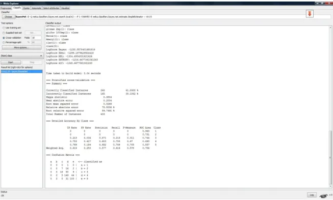
3.1.2.1 Bayes Network Classifier

When we applied Bayes Network onto refreshed data, we got the results shown as below on Figure 3.2

Figure 3.2 : Bayes network classifier

As seen correctly classified instances are low (61.8938) because there are so many attributes. Root mean squared error is 0.3266 and it shows the differences between values predicted by the model or the estimator. Confusion matrix shows us the data set is unbalanced and the data gathered in the attributes of 3,4,5. Log scores also given.

(49)

3.1.2.2 BF Tree Decision Tree

This is a module for building a best-first decision tree classifier. This class uses binary split for both nominal and numeric attributes. For missing values, the method of 'fractional' instances is used. This method used for pre-steps of bayes.

When we applied BF Tree onto refreshed data, we got the results shown as below on Figure 3.3.

Figure 3.3 : Best-first decision tree

In this first decision tree, size is 93 and number of leaves are 47. This tree shows how weka determines the attributes to be classified. It shows the attributes range to decide and relations between them. In this tree correctly classified instances are 258 (%59.54) the reason of this low classification is there are so many attributes. Root mean squared error is 0.3402.

(50)

3.2 Rosetta Rough Set

3.2.1 Preprocessing

We manually preprocessed the data in MS-Notepad and through PERL scripts. This was done to remove unwanted space between the attribute values, and to insert attribute types and Undefined for missing values in the Rosetta input file.

The model used in AutoClass in the experiments to follow was Single multinomial. All attributes were treated as discrete values. The reason for this is that AutoClass expects a zero-point and a relative error for scalars. By using discrete values, we were able to make the input more similar to the input to Rosetta. The datasets were preprocessed in Rosetta and the splits used in Rosetta were exported using cut and pasted into MS-Notepad.

3.2.2 Experiment

We manually read the archives and chose the attributes that we thought had some possible functional dependencies. The attributes, with explanation are listed in Table 2.3.

When we manually inspected the data we found that the values in attributes Glucopaghe and Insulin Lantus were mostly missing, so we removed them. We also removed three objects out of 470 that had most of the attribute values missing. table below shows the number of objects and attributes in the dataset of experiment. Table 3.1: Facts on Experiment data set.

Name Object Attributes Obj.w/miss val.

Rought set 470 18 156

Benchmarking data mining techniques for segmenting diabetes patients

T.C.

BAHÇEŞEHİR ÜNİVERSİTESİ

BENCHMARKING DATA MINING TECHNIQUES FOR SEGMENTING

DIABETES PATIENTS

İnayet ADALI

T.C

BAHÇEŞEHİR ÜNİVERSİTESİ

INSTITUTE OF SCIENCES

COMPUTER ENGINEERING

BENCHMARKING DATA MINING TECHNIQUES FOR SEGMENTING

DIABETES PATIENTS

İnayet ADALI

Supervisor: ASSOC.PROF.DR. ADEM KARAHOCA

ABSTRACT

BENCHMARKING DATA MINING TECHNIQUES FOR

SEGMENTING DIABETES PATIENTS

ÖZET

TABLE OF CONTENTS

TABLES

FIGURES

ABBREVIATIONS

1. INTRODUCTION

2. MATERIALS & METHODS

 









 

 









 

 























































 







 

 



 

 







 



 



_

_

_

_{ }

_

_

_

_

_

_