Improving application behavior on heterogeneous manycore systems through kernel mapping

IMPROVING APPLICATION BEHAVIOR ON

HETEROGENEOUS MANYCORE SYSTEMS

THROUGH KERNEL MAPPING

A THESIS

SUBMITTED TO THE DEPARTMENT OF COMPUTER ENGINEERING AND THE GRADUATE SCHOOL OF ENGINEERING AND SCIENCE

OF BILKENT UNIVERSITY

IN PARTIAL FULFILLMENT OF THE REQUIREMENTS FOR THE DEGREE OF

MASTER OF SCIENCE

By

¨

Omer Erdil Albayrak

July, 2013

I certify that I have read this thesis and that in my opinion it is fully adequate, in scope and in quality, as a thesis for the degree of Master of Science.

Assoc. Prof. Dr. ¨Ozcan ¨Ozt¨urk (Advisor)

I certify that I have read this thesis and that in my opinion it is fully adequate, in scope and in quality, as a thesis for the degree of Master of Science.

Assoc. Prof. Dr. ˙Ibrahim K¨orpeo˘glu

I certify that I have read this thesis and that in my opinion it is fully adequate, in scope and in quality, as a thesis for the degree of Master of Science.

Asst. Prof. Dr. Alper S¸en

Approved for the Graduate School of Engineering and Sci-ence:

Prof. Dr. Levent Onural Director of the Graduate School

ABSTRACT

IMPROVING APPLICATION BEHAVIOR ON

HETEROGENEOUS MANYCORE SYSTEMS

THROUGH KERNEL MAPPING

¨

Omer Erdil Albayrak M.S. in Computer Engineering Supervisor: Assoc. Prof. Dr. ¨Ozcan ¨Ozt¨urk

July, 2013

Many-core accelerators are being more frequently deployed to improve the system pro-cessing capabilities. In such systems, application mapping must be enhanced to maxi-mize utilization of the underlying architecture. Especially, in graphics processing units (GPUs), mapping kernels that are part of multi-kernel applications has a great impact on overall performance, since kernels may exhibit different characteristics on different CPUs and GPUs. While some kernels run faster on GPUs, others may perform better in CPUs. Thus, heterogeneous execution may yield better performance than executing the application only on a CPU or only on a GPU. In this thesis, we investigate on two approaches: a novel profiling-based adaptive kernel mapping algorithm to assign each kernel of an application to the proper device, and a Mixed Integer Programming (MIP) implementation to determine optimal mapping. We utilize profiling information for kernels on different devices and generate a map that identifies which kernel should run where in order to improve the overall performance or energy consumption of an appli-cation. Initial experiments show that our approach can efficiently map kernels on CPUs and GPUs, and outperforms CPU-only and GPU-only approaches. Some part of this work is published in 41st International Conference on Parallel Processing Workshops (ICPPW), 2012 [1], and submitted to Parallel Computing journal (ParCo) [2].

Keywords: Mixed Integer Programming, Kernel Mapping, Heterogeneous Systems, GPGPU, OpenCL.

¨

OZET

ETK˙IL˙I C

¸ EK˙IRDEK FONKS˙IYON DA ˘

GILIMI ˙ILE

HETEROJEN C

¸ OK C

¸ EK˙IRDEKL˙I S˙ISTEMLERDE

UYGULAMA DAVRANIS¸LARININ ˙IY˙ILES¸T˙IR˙ILMES˙I

¨

Omer Erdil Albayrak

Bilgisayar M¨uhendisli˘gi, Y¨uksek Lisans Tez Y¨oneticisi: Doc¸. Dr. ¨Ozcan ¨Ozt¨urk

Temmuz, 2013

Her gec¸en g¨un sistemlerin is¸lem kapasitelerini artırmak ic¸in, daha fazla c¸ok-c¸ekirdekli hızlandırıcı piyasaya sunulmaktadır. Bu gibi sistemlerde, uygulamaların var olan donanım mimarisi ile es¸les¸tirilmesi is¸lemi daha fazla ¨onem kazanmak-tadır. C¸ ¨unk¨u, daha uygun es¸les¸tirmeler sonucunda donanımdan kazanılan faydanın arttırılması hedeflenmektedir. ¨Ozellikle grafik is¸leme birimlerinde, c¸ekirdek fonksiy-onların donanıma do˘gru bir s¸ekilde es¸les¸tirilmesinin nihai performans ¨uzerine etk-isi b¨uy¨ukt¨ur. Bunun nedeni, c¸es¸itli c¸ekirdek fonksiyonlarn c¸es¸itli karakteristiksel ¨ozelliklere sahip olmalarıdır. Bu karakteristiksel ¨ozellikler nedeniyle bazı fonksiy-onlar merkezi is¸lem biriminde (CPU) iyi sonuc¸lar verirken, ¨otekiler ise grafik is¸leme birimlerinde (GPU) daha iyi performans sonuc¸ları ortaya koymaktadırlar. Bu ne-denle, uygulamaların heterojen ortamlarda heterojen bir s¸ekilde c¸alıs¸tırılması, uygu-lamanın sadece CPU ya da sadece GPU ¨uzerinde c¸alıs¸tırılmasından daha iyi per-formans sonuc¸ları verecektir. Bu tezde iki farklı yaklas¸ım aras¸tırılmıs¸tır: ilki, c¸ekirdekleri uygun aygıta atamak ic¸in gelis¸tirdi˘gimiz ¨ozg¨un profil temelli uyarlan-abilir c¸ekirdek es¸les¸tirme algoritması, ve ikincisi, ideal es¸les¸tirmeleri bulmak ic¸in ¨uretti˘gimiz karıs¸ık tamsayılı programlama modelidir. Gelis¸tirdi˘gimiz algoritmada, bir uygulamanın nihai performansını artırmak ya da enerji t¨uketimi azaltmak hedeflen-mektedir. Bu hedef do˘grultusunda uygulamaların c¸ekirdek fonksiyonlarının do˘gru bir s¸ekilde aygıtlara da˘gılımı yapılmakta, ve bu is¸lem s¨uresince c¸ekirdek fonsiyonların sistemde bulunan c¸es¸itli aygıtlar ¨uzerinde elde edilen profil bilgileri kullanılmaktadır. Deneyler g¨ostermektedir ki, yaklas¸ımlarımız verimli bir s¸ekilde c¸ekirdek fonksiyon-ların CPU’lara ve GPU’lara da˘gılımını yapmakta, ve sadece CPU ya da sadece GPU yaklas¸ımlarından daha iyi sonuc¸lar ortaya koymaktadır. Bu tezde bahsi gec¸en is¸in bir b¨ol¨um¨u 41. Uluslararası Paralel ˙Is¸leme C¸ alıs¸tayında (ICPPW, 2012) yayınlanmıs¸ [1], ve Paralel Hesaplama dergisine (ParCo) g¨onderilmis¸tir [2].

v

Anahtar s¨ozc¨ukler: Karıs¸ık Tamsayılı Programlama, C¸ ekirdek Es¸les¸tirme, Heterojen Sistemler, GPGPU, OpenCL.

Acknowledgement

I would like to express my gratitude to my supervisor Assoc. Prof. Dr. ¨Ozcan ¨Ozt¨urk who has been supporting me for the last four years. He was not only an academic advisor, but also an idol especially in work discipline, and ethics. It has always been an honor and pleasure to be his student.

This thesis could not be completed without the advices and supports of ˙Ismail Akt¨urk, I would like to thank him in name.

I would like to thank to Assoc. Prof. Dr. ˙Ibrahim K¨orpeo˘glu and Asst. Prof. Dr. Alper S¸en for accepting to read and review the thesis.

I would like to acknowledge Asst. Prof. Dr. Ka˘gan G¨okbayrak for his much-appreciated help in developing the MIP formulation, and also for the solver environ-ment.

I also would like to thank to Assoc. Prof. Dr. U˘gur G¨ud¨ukbay and William Sawyer for leading me to a great academic life.

I would like to thank to ¨Ozge Koc¸ for her love and support. One glimpse of her takes away all the sorrow.

I would like to thank to C¸ a˘glar and Yi˘git, without them the last three years would become such a misery, I would like to thank them in name.

I would like to thank The Scientific and Technological Research Council of Turkey (T ¨UB˙ITAK), especially Kamil, Ahmet, Mehmet, Tu˘gc¸e, ¨Umit, Alptu˘g and all of my colleagues for their support.

Finally, I would like to offer my sincere love to my family, Talat, Deniz and Erdinc¸ for their endless support, my grandparents Melek and Emine for their love and my uncle Cengiz for being an idol, and leading me to computer engineering.

Contents

1 Introduction 1

2 Background Information 4

2.1 Multi-Core and Many-Core Systems . . . 4

2.2 GPGPU . . . 9 2.2.1 CUDA . . . 11 2.2.2 OpenCL . . . 11 2.2.3 Kernels . . . 13 2.2.4 Memory Model . . . 13 2.2.5 Execution Grid . . . 15 2.3 Mixed-Integer Programming . . . 17 2.4 Related Work . . . 18 3 Methods 20 3.1 Preliminaries . . . 20 3.2 Our Approach . . . 21

CONTENTS viii

3.3 Greedy Mapping Algorithm . . . 22

3.3.1 Base Algorithm . . . 22

3.3.2 Improved Algorithm . . . 26

3.4 Multi-Device Mapping . . . 30

3.5 Mixed-Integer Programming . . . 33

3.6 Different Types of Cost Functions . . . 37

4 Experimental Results 39 4.1 Setup . . . 39

4.2 Results . . . 40

4.2.1 Greedy Algorithm Results . . . 42

4.2.2 MIP Results . . . 43

4.2.3 Analysis of Data Transfer Cost On Overall Kernel Mapping . 45 4.2.4 Reducing Energy Consumption Through Effective Kernel Mapping . . . 46

List of Figures

2.1 Uniprocessor power consumption by the years. The latest processors such as Pentium 4 and Itanium had great power needs [3]. . . 5

2.2 GPU architectures usually have many simple compute units (green squares), CPU architectures, in contrast, have less number of complex compute units[4]. . . 6

2.3 GPU and CPU comparison in terms of Gflops over years. As can be seen, recently developed GPUs provide much more Gflops capacity over years and the gap between CPUs and GPUs is increasing[4]. . . 7

2.4 GPU and CPU comparison in terms of memory bandwidth over years. As can be seen, GPUs have four times more bandwidth when com-pared to CPUs, thus the data transfer rate from main memory to GPU is much faster[4]. . . 8

2.5 Memory hierarchy in a typical CPU-GPU system. . . 9

2.6 CUDA computing framework stands right between the application and the NVIDIA hardware in the process of porting CUDA parallel appli-cation to the GPU[4]. . . 11

2.7 Sample CUDA kernel. . . 12

LIST OF FIGURES x

2.9 CUDA execution grid splits the workforce into blocks and each block is divided into threads[4]. . . 15

2.10 OpenCL execution grid similar to CUDA[5]. . . 16

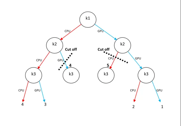
2.11 Branch and bound algorithm in action on the recursion tree. Note that, calculations happen from in left to right. . . 17

3.1 High level view of our approach. . . 22

3.2 Time cost function calculation in action. Cost of running a kernel for each device is calculated according to the Equations 3.1 and 3.2. Note that, CPU is referred as Host and GPU is referred as Device. Therefore, Host to Host(H2H) and Device to Device (D2D) is always zero due to the fact that they mean the data objects stay in the same device. . . 25

3.3 Illustration of mapping obtained by base algorithm applied to the sam-ple problem given in 3.1. Note that, the total cost with the base algo-rithm is 15. . . 27

3.4 Illustration of mapping obtained when kernel1 is forced to execute on the GPU for the sample problem given in Table 3.1. Note that, the cost of kernel1 for CPU and GPU are 5 and 6, respectively. However, when kernel1 is forced to execute on the GPU (which is not the local minimum) the total cost is reduced to 14. . . 28

4.1 Comparison of GPU-only, CPU-only, base (GA), and improved algo-rithm (IA) mappings. . . 42

4.2 Comparison of GPU-only, CPU-only, improved algorithm (IA), and MIP implementation mappings. . . 44

4.3 Speed up of benchmarks normalized with respect to the best CPU-only or GPU-only. . . 44

LIST OF FIGURES xi

4.4 Comparision of the execution times of each algorithm. Note that, for 10000 kernels MIP model couldn’t generate the mapping due to insuf-ficient amount of memory. . . 45

4.5 Speed up of benchmarks normalized with respect to the best single-device execution with different data transfer times. Note that, the map-ping also changes according to the data transfer times. . . 47

4.6 Speed up of benchmarks normalized with respect to the default data transfer times with varying data transfer times. . . 47

4.7 Comparison of time × power cost function for each kernel mapping. Values are normalized with respect to the best single-device execution. 48

4.8 Execution latency values for each mapping given in Figure 4.7. Note that, these are normalized with respect to the best single-device execu-tion. . . 48

4.9 Comparison of time × power2cost function for each kernel mapping. Values are normalized with respect to the best single-device execution. 50

4.10 Execution latency of each mapping given in Figure 4.9. Note that, these values are normalized with respect to the best single-device exe-cution. . . 50

List of Tables

3.1 A simple example to show the difference between GA and IA. . . 26

3.2 Sample data for multi device mapping. Each column shows the execu-tion time of kernels on the corresponding device. . . 31

3.3 Trace data for running the base algorithm on the sample data given in Table 3.2. Note that, the data transfer cost for each transfer is two. If the transfer cost is added to the execution latency, the sum operation is shown in the cost column of each device. . . 32

3.4 Trace data for running the base algorithm on the sample data given in Table 3.2. Note that, the data transfer cost for each transfer is two. Cost column shows the decision cost for running the the kernel k on each device. . . 33

4.1 Our experimental setup and hardware components. . . 39

4.2 The descriptions and problem sizes of benchmarks used in our experi-ments [6, 7]. . . 40

4.3 Distribution of kernels with different approaches. . . 41

4.4 Execution times of benchmarks with different approaches. . . 41

LIST OF TABLES xiii

Chapter 1

Introduction

Today’s high performance and parallel computing systems consist of different types of accelerators, such as Application-Specific Integrated Circuits (ASICs) [8], Field Pro-grammable Gate Arrays (FPGAs) [9], Graphics Processing Units (GPUs) [10], and Accelerated Processing Units (APUs) [11]. In addition to the variety of accelerators in these systems, applications that are running on these systems also have different pro-cessing, memory, communication, and storage requirements. Even a single application may exhibit different such requirements throughout its execution. Thus, leveraging the provided computational power and tailoring the usage of resources based on the appli-cation’s execution characteristics is immensely important to maximize both application performance and resource utilization.

Applications running on heterogeneous platforms are usually composed of multi-ple exclusive regions known as kernels. Efficient mapping of these kernels onto the available computing resources is challenging due to the variation in characteristics and requirements of these kernels. For example, each kernel has a different execution time and memory performance on different devices. It is our goal to generate a kernel map-ping system that takes the characteristics of each kernel and their dependencies into account, leading to improved performance.

In this thesis, we propose a novel adaptive profiling-based kernel mapping algo-rithm for multi-kernel applications running on heterogeneous platforms. Specifically,

we run and analyze each application on every device (CPUs and GPUs) in the system to collect necessary information, including kernel execution time and input/output data transfer time. We, then, pass this information to a solver to determine the mapping of each kernel on the heterogeneous system. Solvers used are a greedy algorithm (GA) based solver, an improved version of the same algorithm (IA), and a Mixed-Integer Programming (MIP) based solver. Our specific contributions are:

• an off-line profiling analysis to extract kernel characteristics of applications.

• an adaptive greedy algorithm (GA) to select the suitable device for a kernel con-sidering its execution time and data requirements.

• an improved version of the greedy algorithm (IA) to avoid getting stuck in local minima.

• a Mixed-Integer Programming (MIP) implementation to determine optimal map-ping and to compare it with the greedy approach.

• specific cost functions targeting the energy consumption, besides overall execu-tion delay of an applicaexecu-tion.

The initial results revealed that our approach increases the performance of an ap-plication considerably compared to a CPU-only or GPU-only approach. Furthermore, in many cases, our generated mappings are equivalent to the mappings of MIP imple-mentations, or very close to them. Although our initial experiments are limited to a single type of CPU and GPU, it is possible to extend this work to support multiple CPUs, GPUs, and other types of accelerators. Moreover, the proposed algorithm can be modified with different cost functions to enhance different properties of an applica-tion, such as energy consumption.

The remainder of this thesis is organized as follows. Background information is discussed in Chapter 2. Specifically, GPGPU concept is given in Section 2.1. Related work on general-purpose GPU computing (GPGPU) is given in Section 2.4. The prob-lem definition and an introduction to the proposed approach are given in Section 3.1. The details of the greedy algorithm (GA) and the implementation are given in Sec-tion 3.3. The multi-device mapping is given in SecSec-tion 3.4. The MIP formulaSec-tion is

introduced in Section 3.5. The different cost functions concerning energy consump-tion are given in Secconsump-tion 3.6. The experimental evaluaconsump-tions are presented in Chapter 4. Finally, we present conclusion and future work in Chapter 5.

Chapter 2

Background Information

2.1

Multi-Core and Many-Core Systems

Multi-Core processor is a single computing device with two or more independent, yet connected central processing units (called ”cores” or ”processing elements”). By the late 1990’s manufacturers discovered that improvements on the manufacturing tech-niques and the chip design had diminishing return on performance gain. According to Gordon E. Moore (co-founder of Intel), between 1958 and 1965 every year the amount of transistors doubled [12] and he expected this trend to go on at least for an-other 10 years. In fact, this trend continued until late 90’s, however, with the increase in the number of transistors, energy consumption and heating problems became con-siderably difficult. Also, the performance gain was not as high as ten, twenty years ago. Therefore, in 2000’s manufacturers head towards the multi-core systems. In early 2000’s commodity dual-core systems emerged and in 10 years, the number of process-ing elements quadrupled. Nowadays, many-core systems with hundreds of processprocess-ing elements are being deployed.

The multi-core processors have architectural advantages over uniprocessors (only one processing element in each die). Because, in order to increase the performance of a uniprocessor, one must increase the frequency, transistor amount and energy. On the other hand, to enhance the performance of a multi-core system, increasing the number

Figure 2.1: Uniprocessor power consumption by the years. The latest processors such as Pentium 4 and Itanium had great power needs [3].

of cores in a die is sufficient most of the time. Increasing the number of cores may seem to be more energy hungry. However, multi-core systems can dynamically adjust the number of active cores to increase the energy efficiency. Thus, in need of processing power, all of the processors may be activated to increase the performance or vice versa. Moreover, multi-cores also help to cope with the heating problem which is one of the biggest concerns of uniprocessors.

Traditionally, there are two types of multi-core architectures, homogeneous and heterogeneous. Homogeneous architectures consist of some number of simple, power efficient processing elements. In this context, simple means individually not as pow-erful as uniprocessors, yet effective when working together collaboratively. Intel and AMD commodity CPU’s can be given as examples to homogeneous architectures. On the other hand, heterogeneous architectures consist of few big, powerful units with many simple, efficient processing elements. Traditionally, in heterogeneous systems, the number of powerful elements are less than the simpler ones, the job of powerful

Figure 2.2: GPU architectures usually have many simple compute units (green squares), CPU architectures, in contrast, have less number of complex compute units[4].

elements is to manage the small processing elements, and also to contribute to compu-tation when it is needed. The major examples of heterogeneous architectures are IBM Cell, IBM Xenon CPUs, and GPUs.

Graphics Processing Units (GPUs) are a variation of CPUs specialized for the graphics domain. They are the extreme case of many-core architecture. Traditionally, a graphical application requires high amount of mathematical computation. There-fore, GPUs are designed in a way that they can cope with high number of calculations on immense amount of data. To cope with such workload, GPUs utilize instruction level parallelism, data level parallelism and pipelining. Currently, the state of the art GPUs are very powerful. For example, NVIDIA Titan [13] has 2688 computing units and a 6GB integrated memory working at 6.0 Gbps, and it only requires 250 Watt power. Moreover, it can handle 4,494 GFLOPS (giga-floating operations per second). On the other hand, a state of the art CPU such as, Intel i7-3960x [14] has only 6 computing units, which can handle 12 threads simultaneously with hyper-threading technology [15], and it can only handle 187 Gflops [16] and requires 130 Watt.

Such architectural diversity comes from the requirements of the tasks which these devices are assigned to. GPUs are designed to handle intense mathematical com-putation on immense amount of data. Which is exactly what graphics rendering is about. Therefore, GPUs don’t need complex hardware structures, the computing units in GPUs are small and less powerful, yet very effective when in great numbers. That is

Figure 2.3: GPU and CPU comparison in terms of Gflops over years. As can be seen, recently developed GPUs provide much more Gflops capacity over years and the gap between CPUs and GPUs is increasing[4].

why the number of computing units in a GPU is much higher than a traditional CPU. On the other hand, CPUs deal with not only mathematical calculations, but also I/O op-erations, encryption/decryption, encoding/decoding and many other additional tasks. Such additional capabilities require specialized sub-components, thus some space in CPU chip is reserved for the additional hardware. As a result, CPUs end up with big, powerful, multi-functional computing devices in small numbers. An example is shown in Figure 2.2, where a GPU with many small compute units and a smaller cache and control units. On the other hand, CPU has just four compute units and much bigger control unit and cache per compute unit.

GPU architecture is more suitable for data-parallel computations because of the tremendous computational horsepower (Figure 2.3) and memory bandwidth (Fig-ure 2.4). For a typical graphics rendering, for each vertex and edge, there is a pipeline

Figure 2.4: GPU and CPU comparison in terms of memory bandwidth over years. As can be seen, GPUs have four times more bandwidth when compared to CPUs, thus the data transfer rate from main memory to GPU is much faster[4].

of several computations, such as shading, lighting, screen clipping, z-buffer elimina-tion and many more operaelimina-tions. This pipeline is applied to billions of vertices and edges on the screen at least for 25-30 times per second. Therefore, GPU architecture is specialized to handle such data intensive and parallel computational mechanism. Figure 2.3 shows the GFLOPS (one thousand floating point operations per second) ca-pacity of current GPUs. As can be seen in the figure, latest GPUs have a caca-pacity to handle six times more floating point operations per second than the latest CPUs.

GPUs also have much higher memory bandwidth as shown in Figure 2.4. However, this bandwidth is between the compute units and the internal memory. Unfortunately, the external bandwidth between main memory and the graphics card is bounded by the main board’s data bandwidth, and it is much lower than the internal transfer rate. Therefore, although the data transfer internally is fast, the cost of data transfer to the

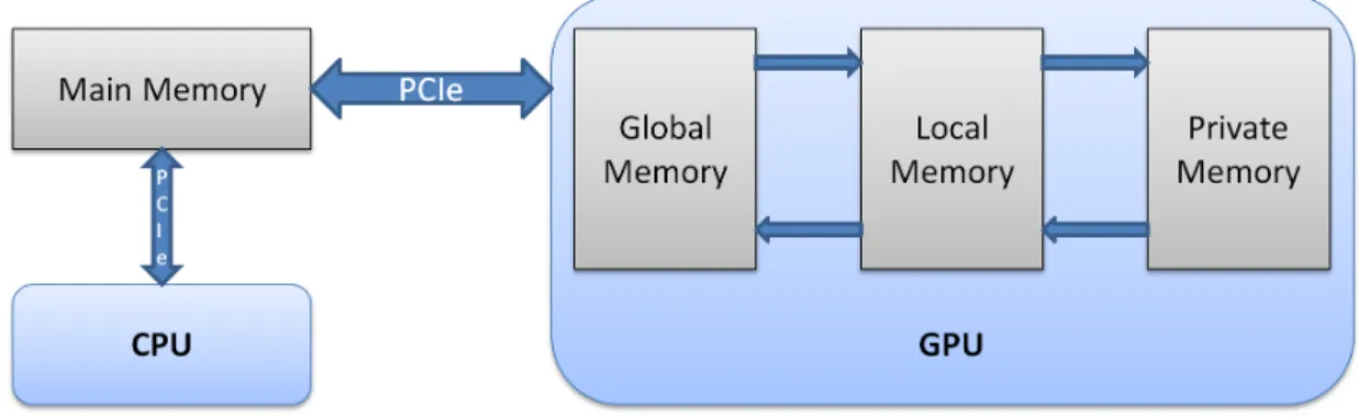
Figure 2.5: Memory hierarchy in a typical CPU-GPU system.

graphics card beforehand is considerably high.

2.2

GPGPU

General Purpose Computing on Graphics Processing Units (GPGPU) is the utilization of a graphics processing unit (GPU), which normally handles only graphics render-ing computations, to perform massively data-parallel computations which normally handled by a CPU. As explained in Chapter 2.1, GPUs have a great structure for data-parallel operations due to its immense computation power shown in Figure 2.3, and internal memory bandwidth shown in Figure 2.4. As discussed in Section 4.2, for some algorithms, GPUs may execute faster than its parallel implementation for CPU. There are even much better improvements, yet they are not in the scope of this the-sis. According to TOP 500, an organizational website which keeps track of the TOP 500 supercomputers on earth, the most used accelerators and co-processors used in supercomputers are by far the GPUs [17].

Alongside its performance benefits, GPUs are very energy efficient devices. Ac-cording to researches conducted by NVIDIA, the most efficient CPU require 10 times more energy than a GPU [18]. In addition, Bloomberg swapped out their systems run-ning on 2000 CPUs with 48 NVIDIA Tesla GPUs and their annual energy cost backed from $1.2 million to $30,000 [18]. Similarly, French bank BNP Paribass changed 64 CPUs with a pair of GPUs and the new configuration cut energy use from 44 kilowatts

to 2.9 kilowatts [18]. As also explained in Chapter 2.1, GPUs require much less energy per GFLOPS compared to a typical CPU.

Despite the fact that GPUs may end up with much better results and energy effi-ciency, the complex internal memory structure of GPUs complicate the software devel-opment, especially from CPU optimized implementations. Figure 2.5 shows a simple illustration of GPU and main memory structures together. In the figure ”GLOBAL”, ”LOCAL” and ”PRIVATE” corresponds to the three major internal memory structures of a GPU and ”PCIe” is the bus between the graphics card and the main memory. Since, there is multi-level memory hierarchy in GPU, a data object must be moved be-tween each level, and each level has different characteristics. While, private memory is the fastest and the closest to computing units, global memory is both the slowest and the furthest memory level. Local memory is in between global and private memories in terms of distance and data transfer rate. In order to be processed, a data object must follow a path from the main memory via global and local memories and ends up in the private memory. Therefore, multi-level memory structure of GPUs requires well optimization and utilization of each level. In order to obtain the best results from a GPU, it is necessary to have an in-depth understanding of the GPU structure. This, in turn, makes legacy code porting a non-trivial task.

There are two major GPGPU platforms accepted by the community right now, and these are CUDA and OpenCL. CUDA is the GPGPU platform developed for only NVIDIA graphics cards by NVIDIA, thus it is supported by only NVIDIA. OpenCL stands for Open Computing Library, and it is a framework for parallel programs that execute across heterogeneous platforms consisting of CPUs, GPUs, APUs and other processors. It has been adopted and supported by many companies, such as AMD, Intel, NVIDIA, ARM, Apple, and many others. CUDA is discussed in detail in Chap-ter 2.2.1. Likewise, OpenCL is discussed in detail in ChapChap-ter 2.2.2. ChapChap-ter

Figure 2.6: CUDA computing framework stands right between the application and the NVIDIA hardware in the process of porting CUDA parallel application to the GPU[4].

2.2.1

CUDA

CUDA is a programming model for utilization of NVIDIA graphics cards for general purpose applications. Sample works indicate that the adaptation of computation inten-sive applications to the GPU systems via CUDA framework result in great performance benefits [19, 20, 21]. This difference comes from the reasons discussed in Chapter 2.2. Figure 2.6 shows the CUDA framework itself, the libraries, and the drivers which stand right between the application and the hardware.

2.2.2

OpenCL

OpenCL is also a programming model for utilization of various hardware. OpenCL is a framework for developing applications that run across heterogeneous systems consist-ing of CPUs, GPUs, APUs, FPGAs, mobile devices, etc. from various manufacturers. In fact, OpenCL is just like CUDA, targetting the additional hardware to utilize. How-ever, it is not limiter to only GPUs. OpenCL is supported by a non-profit technology consortium, Khronos Group [22], formed by members from different companies such

Figure 2.7: Sample CUDA kernel.

as, Apple, AMD, Intel, NVIDIA, ARM, etc. The main goal of OpenCL is to enable users to develop hardware-independent programs. Therefore, OpenCL applications can utilize various devices from various manufacturers. Additionally, such feature also enables to develop heterogeneous platforms. Portions of the computations can be as-signed to different computing devices, and performance gain can be achieved. The work proposed in this thesis supports such idea of performance gain via heterogeneous computing.

OpenCL framework consists of several layers: application, OpenCL runtime, OpenCL platform, and installable client driver (ICD). Application, runtime, platform layers are similar to the components of CUDA framework. On the other hand, instal-lable client driver is the main difference in OpenCL. Instalinstal-lable client driver controls the porting mechanism of each application to the target hardware. Each manufacturer deploys an ICD for their own products. Therefore, the porting mechanism is controlled by the manufacturer to acquire the best performance of the hardware.

2.2.3

Kernels

Kernels are the functions that run on the hardware. Each kernel consists of three crit-ical sections which are, thread access model, memory access model, and finally the operation itself. Thread access model is the assignment of the threads to the data ob-jects (or buffers). Figure 2.7 shows a sample CUDA kernel. In this code snippet, two dimensional thread model is defined. Each thread dimension has one to one relation with the dimensions of the data objects. Serial applications would define two levels of indices to access each data object, and iterating over these indices, the data would be processed. However, for the parallelization of this operation, each index is assigned to a thread, and each thread concurrently processes a part of the data objects. The ex-ecuted device code is stated with the ” global ” keyword which means the function runs on the device, and it is accessable from the host code (main function). Finally, the actual operation in Figure 2.7 is the sum operation over each index of the data objects A and B, and the result is written to the corresponding C index and sent back to the main memory.

2.2.4

Memory Model

A GPU architecture has multiple levels of memory, these memory levels, from outer-most to inner-outer-most, are called global memory, shared memory, local memory and reg-isters, while each memory has different access times and different needs. The underly-ing reasons for such complex memory model is discussed in Chapter 2.2.5. Figure 2.8 illustrates the memory architecture. Each memory level has different access times due to the distance to threads. The closest one is also the fastest and the smallest in terms of capacity. When a data object is sent to GPU from CPU, it is first placed in the global memory (or similar). When threads need to access the data objects, each block fetches a portion of the data to its own shared memory, where the threads of that particular block will work on. Similarly, each thread fetches its own data to its own local mem-ory from the block’s shared memmem-ory. When the processing is completed, each data set is sent back to global memory, and finally to the CPU. This way, it is possible to execute the threads much faster from a local memory. However, data transfer costs can

Figure 2.8: Multiple layers of memory in GPU[4].

be significant if there is not sufficient computation required.

Moreover, there are additional fast and efficient memory types, such as texture memory, and constant memory. These additional memories are read-only memory types and data can be sent only on the setup phase, also the capacity of these structures are too small to fit all the input data. However, since they are fast and effective, the constant read-only data can be copied and used without conflicting the threads.

2.2.5

Execution Grid

GPUs are designed to be able to cope with huge amount of data and computation at the same time. Therefore, GPUs must have a mechanism to separate different compu-tations from each other. For this purpose, computation units are assembled in chunks, and each chunk is assigned to a set of operations and data. These chunks are called Streaming Multiprocessor (SM) and each processing element or computation unit is called Streaming Processor (SP). This structure enables applications to run different tasks for each SM, however the application itself must be clever enough to compre-hend in which chunk it exists.

Figure 2.9: CUDA execution grid splits the workforce into blocks and each block is divided into threads[4].

Figure 2.10: OpenCL execution grid similar to CUDA[5].

GPGPU frameworks offer an execution grid to the user. Figure 2.9 and Figure 2.10 shows the execution grids for CUDA and OpenCL platforms. Each block in CUDA (work-group in OpenCL) is assigned to an SM. Each thread (work-item in OpenCL) is assigned to a SP. Moreover, such multiple level hierarchy provides the utilization of the memory model discussed in Chapter 2.2.4. Figure 2.8 shows the memory model discussed earlier, each SM has its own shared memory and for each SP a local mem-ory is dedicated. Each thread (work-item in OpenCL) must move its own data to the shared and local memory. Therefore, blocks or work-groups must be composed of threads working on the same section of the data objects in order to utilize the shared memory. The most significant advantage of such hierarchy is that it enables the user to implement a pipeline of operations which has a different memory access model. To explain, one set of SMs may require to access column-wise for one type of operation and another set may need to access row-wise, therefore with this architecture each set may be assigned to different SMs.

Cut off Cut off 4 5 GPU 4 3 GPU GPU GPU GPU CPU CPU CPU CPU CPU k3 k2 k2 k1 k3 k3 k3 2 1

Figure 2.11: Branch and bound algorithm in action on the recursion tree. Note that, calculations happen from in left to right.

2.3

Mixed-Integer Programming

Integer Linear Programming (ILP) is a mathematical optimization method for finding the best solution for a problem, such as the minimum delay, or maximum profit. A set of integer or boolean values are given as linear relations to the ILP optimization method, and the method itself effectively searches for the best outcome. The optimiza-tion problem itself is an NP-hard problem, yet ILP technique effectively solves. The relations between the variables define an N-dimensional space and the method finds a point in the space by cutting down each dimension. If the variables used in the mathe-matical model are all integers, then the problem is called Integer Linear Programming (ILP), otherwise it is called Mixed-Integer Programming (MIP). The mathematical model of the optimization problem we implemented has both integer and non-integer values, therefore the optimization method we used in this work will be referred as Mixed-Integer Problem (MIP) in the rest of the thesis.

There are several algorithms to solve linear problems, such as branch and bound [23] and cutting-plane method [24]. The tool we used to solve our problem applies the branch and bound algorithm. This algorithm starts searching a tree of vari-ables recursively and calculates the potential outcomes. Whenever it finds a better combination of variables the setting becomes the local optimum. For the rest of the tree, whenever the local cost passes the local optimum, the algorithm cuts down the rest of the tree and reverts to a past decision and continues searching. At the very end, after all the branches are cut-off or searched, it locates the global optimum.

In Figure 2.11 a sample branch and bound is explained. The circles correspond to an OpenCL kernel, and for each kernel there are two possibilities to work on, CPU and GPU. Each arrow indicates the local cost in the search tree. The algorithms starts from the left branch and finds the local minimum as 4, then it moves to the next leaf with cost 3, and finds out that there is a better option with smaller cost, as a result, the local optimum becomes 3. Afterwards, the algorithm moves on to k2 with GPU setting, and since the cost of this decision is already 4, the branch is cut-off. Algorithm reverts to k1 and continues the search, where eventually after skipping couple of branches, finds the global optimum in ”all GPU” setting.

2.4

Related Work

OpenCL is an open standard for parallel programming, targeting heterogeneous sys-tems [22]. It began as an open alternative to Brook [25], IBM CELL [26], AMD Stream [27], and CUDA [28]. It provides a standard API that can be employed on many architectures regardless of their characteristics, and therefore has become widely accepted and supported by major vendors. In this work, we also used OpenCL and evaluated our approach on an OpenCL version of the NAS benchmarks [7].

Recent advancement in chip manufacturing technology has made it feasible to pro-duce power efficient and highly parallel processors and accelerators. This, however, increases the heterogeneity of the computing platforms and makes it challenging to determine where to run the given application. To the best of our knowledge, there are

only a few studies targeting this critical challenge. Luk et al. proposed Qilin [29], which uses a statistical approach to predict kernel execution times offline, generate a mapping and perform the execution. Rather than individual kernel mapping, they par-tition single instruction multiple data (SIMD) operations into sub-operations and map these sub-operations to the devices. In contrast to Qilin, we aim to map the kernels as a whole rather than their sub-operations. While we obtain CPU and GPU execu-tion times (in addiexecu-tion to the data transfer times) through profiling, they use statistical regression model to estimate these values. Therefore, it is orthogonal to our profiling method, and can be integrated into our system when profiling is not possible or when it is costly.

Grewe and O’Boyle [30] proposed a machine learning-based task mapping algo-rithm. They use a predictor to partition tasks on heterogeneous systems. Their method predicts the target device for each task according to the extracted code features used in the training set of the machine-learning algorithm. Our decision method could be enhanced with such techniques in the future.

The main difference between these works and ours is that ours is an adaptive profiling-based kernel mapping algorithm.

Chapter 3

Methods

3.1

Preliminaries

A major challenge in a heterogeneous platform is using existing resources while ob-taining an application’s highest performance. This issue is mainly due to the nature of such systems, because they comprise computing devices with different characteristics and capabilities. Therefore, the main goal of this work is to utilize these devices by capturing tasks’ specific characteristics and making task-assignment decisions in a way that tasks are assigned to the device they perform better. Ultimately, the overall perfor-mance will be improved and the underlying resources will be utilized. Traditionally, applications run on a single hardware which they perform better. However, when the application is divided into tasks, each task is assigned to a device, thereby improving the overall performance.

Formally, a kernel mapping problem can be defined as a triplet M AP = {K, D, S} where K is a set of kernels K = {k1, k2, k3, . . . , kn}, D is a set of devices which

kernels can execute on D = {d1, d2, d3, . . . , dm}, and S = {s1, s2, s3, . . . , st} is a data

object set used by kernels. Each kernel ka ∈ K is sequentially executed on a device

db ∈ D right after kernel ki−1and the required data objects sc ∈ S are copied to local

For this thesis, we use a simple heterogeneous platform with a single type of CPU and GPU. However, in reality, a heterogeneous platform may consist of multiple types of CPUs, GPUs, and APUs from different vendors with different features [31, 32, 33]. For example, it is possible to have an NVIDIA GPU and an AMD GPU in the same system. While NVIDIA GPUs are good for simple parallel multi-threaded computa-tions, AMD GPUs are better in vector operations [34, 5]. Thus, the characteristics of a task, such as the number of vector operations and the number of threads running in parallel, become critical while deciding where to run the given application.

Similarly, the size of data required by an application is an important issue, because some of the devices, such as GPUs, may have limited memory space. Therefore, even though an application may be developed targeting a GPU, it may not be possible to execute it on a given GPU because of the limitation on memory.

In addition to kernel characteristics and device specifications, dependencies be-tween kernels are also of concern. Running dependent kernels in two different devices requires data movement upon depended kernels to finish the execution. Hence, for certain mappings it is necessary to consider data transfer costs while assessing the performance of an application.

3.2

Our Approach

Figure 3.1 illustrates, at a high level, how our approach operates. First, we extract the profiling information which is used in kernel mapping.

Specifically, we run and analyze each application on every device (CPUs and GPUs) in the system to collect necessary information, including kernel execution time and input/output data transfer time. As an alternative, we can extract kernel charac-teristics through compiler analysis and employ a machine-learning-based technique, similar to [30], to predict kernel execution times and data transfer overheads. How-ever, this is left as a future work.

Kernel Characteristics Extraction GA Kernel Mapping IA MIP Application

Figure 3.1: High level view of our approach.

Extracted kernel characteristics is subsequently passed to the solver which deter-mines the mapping of each kernel on the heterogeneous system. Specific solvers used are a greedy algorithm (GA) based solver implemented using Java, an improved ver-sion of the greedy solver (IA), and a Mixed-Integer Programming (MIP) based solver implemented on a commercial tool. Our goal in selecting the mapping is to generate a mapping that minimizes the execution cost of each kernel. Note that, depending on the functionality, each device on the system can exhibit different characteristics in terms of data transfer cost, data bandwidth, and performance. This information is crucial for selecting the target device.

3.3

Greedy Mapping Algorithm

3.3.1

Base Algorithm

In this Chapter, we introduce two greedy algorithms mentioned earlier, the base algo-rithm (GA) and its improved version (IA). The main goal of these two algoalgo-rithms are to minimize the overall execution cost via effectively mapping kernels to the devices.

The greedy approach in the base algorithm tries to select the device with the smallest execution time for each kernel. Note that, the base algorithm does not consider the kernel dependencies, therefore it selects the best device for each kernel at the kernel running time. However, due to the complex data dependencies among kernels, mini-mizing the execution cost of each kernel may not minimize the overall performance of an application. Therefore, the dbase algorithm may not yield the best results.

We formulate the CPU and GPU execution times as follows:

CP U costk = CP U runningtimek+ n

X

d=1

DeviceT oHost × InDeviced×

Requiredk,d× sized. (3.1)

GP U costk = GP U runningtimek+ n

X

d=1

HostT oDevice × (1 − InDeviced) ×

Requiredk,d× sized. (3.2)

The first component in each equation indicates the execution time, while the sec-ond component is the data transfer cost. HostToDevice and DeviceToHost functions are simply the data transfer costs from host to device and vice versa. Note that, Requiredk,d is either 1 or 0, and it indicates whether kernel k requires data d. Data

might already be present on the target device, and thus may not need to be moved in. For this purpose, we use InDevicedto indicate whether data d is already in the target

device. Similarly, we express the size of data d using sized. The Figure 3.2 explains

the cost types used during the device selection in a heterogeneous environment. Note that, in Figure 3.2 CPU is referred as Host, since initially buffer objects are located in CPU, and likewise GPU is referred as Device since it is the additional hardware. The sum operation in Expression 3.1 is named as D2H cost (stands for device to host) in the figure, likewise the sum operation in Expression 3.2 is named as H2D cost (stands for host to device). Note that for each buffer object, cost is zero if data is not moved. The kernel execution time for each device is shown as CPU and GPU running times.

Algorithm 1 Base Greedy Algorithm (GA) procedure BASEALGORITHM

total cost = 0 for all Kernel k do

cpu cost = k.CP U T IM E + D2H(k) gpu cost = k.GP U T IM E + H2D(k) if cpu cost < gpu cost then

k.onCpu ← true k.cost ← cpu cost for all Buffer b ∈ k do

b.onCpu ← true end for

else

k.onCpu ← f alse k.cost ← gpu cost for all Buffer b ∈ k do

b.onCpu ← f alse end for

end if

total cost+ = k.cost end forreturn total cost end procedure

procedure H2D(Kernel k) cost = 0

for all Buffer b ∈ k do

if b.onCP U == true then

cost+ = b.H2D transf er cost end if

end for end procedure

procedure D2H(Kernel k) cost = 0

for all Buffer b ∈ k do

if b.onCP U == f alse then cost+ = b.D2H transf er cost end if

end for end procedure

The aforementioned constants are extracted through profiling except InDeviced.

InDeviced is a binary variable and its value depends on the recent iteration of the

algorithm that accessed data d. If data was left in the device after the last access, InDeviced will be 1, otherwise it will be 0. The algorithm assumes that all the data

is initially stored in the CPU, as it is the case in most systems. This assumption can easily be modified to reflect a different system.

The cost of executing kernel k on a particular device is the sum of running time of k on that particular device and the data transfer times for each data object which are required but not on the device.

CPU GPU

Kernel k

Buffer b1 Buffer b2

Kernel k b2 Kernel k

b1 b1 b2

CPU running time GPU running time

D2D cost = 0

H2H cost = 0 H2D cost D2H cost

Running Cost On CPU: CPU running time + D2H Running Cost On GPU: GPU running time + H2D

H2D stands for Host to Device (CPU to GPU) D2H stands for Device to Host (GPU to CPU)

Figure 3.2: Time cost function calculation in action. Cost of running a kernel for each device is calculated according to the Equations 3.1 and 3.2. Note that, CPU is referred as Host and GPU is referred as Device. Therefore, Host to Host (H2H) and Device to Device(D2D) is always zero due to the fact that they mean the data objects stay in the same device.

Kernel CPU GPU Data CPU to GPU GPU to CPU

Number Execution Execution Transfer Transfer

Latency Latency Used Time Time

1 5 4 A 2 2

2 3 2 A 2 2

3 7 6 A 2 0

Table 3.1: A simple example to show the difference between GA and IA.

Algorithm 1 gives the pseudo code for the base algorithm. The base algorithm shown in Figure 3.2 calculates the execution times for both devices according to Equa-tions 3.1 and 3.2 and selects the fastest device for the given kernel. Afterwards, copies each data object to the particular device, and moves to the next kernel. The next kernel calculates the data transfer costs according to the latest states of the data objects. Note that, the assignment of each kernel affects the rest of the kernels, yet the assignment method itself does not consider with the other kernels. Therefore, base algorithm may not give the optimal mapping.

3.3.2

Improved Algorithm

The base algorithm works with most of the tested benchmarks. However, in some cases there is a possibility of getting stuck in local minima due to complex data dependencies among kernels that were not handled in the base algorithm. We proposed the improved algorithm (IA, see Algorithm 2) to avoid such inefficiencies. We introduced the notion of Critical Points, where the algorithm can select the worst target, for the purpose of assessing alternative mappings that may yield better performance. Table 3.1 gives a simple example to show the effect of employing the improved algorithm (IA).

Figure 3.3 illustrates Algorithm 1 running according to the data in Table 3.1. Total cost of running the first kernel on a CPU is calculated as the summation of execution time on the CPU and the data movement cost if data is not currently on the CPU. In our example, data is located in the CPU initially, thereby the total cost of running the first kernel on the CPU is 5 + 0 = 5. Similarly, the total cost of running the first kernel on a GPU is calculated as the summation of the execution time on the GPU and the

CPU GPU Buffer A Buffer A Buffer A Buffer A Kernel 1 Kernel 2 Kernel 3 Cost: 0 _{Cost: 2} Cost: 4 Cost: 5 Cost: 3 Cost: 0 Cost: 2 Cost: 2 Cost: 2 Cost: 6 Cost: 7 Cost: 0 Kernel 2 Kernel 1 Kernel 3 Decision State Decision State Decision State Final State Final State Final State Kernel 1 States Kernel 2 States Kernel 3 States Initial State

Figure 3.3: Illustration of mapping obtained by base algorithm applied to the sample problem given in 3.1. Note that, the total cost with the base algorithm is 15.

CPU GPU Buffer A Buffer A Buffer A Buffer A Kernel 1 Kernel 2 Kernel 3 Cost: 0 _{Cost: 2} Cost: 4 Cost: 5 Cost: 3 Cost: 2 Cost: 0 Cost: 2 Cost: 0 Cost: 6 Cost: 7 Cost: 2 Kernel 2 Kernel 1 Kernel 3 Decision State Decision State Decision State Final State Final State Final State Kernel 1 States Kernel 2 States Kernel 3 States Initial State

Figure 3.4: Illustration of mapping obtained when kernel1 is forced to execute on the GPU for the sample problem given in Table 3.1. Note that, the cost of kernel1 for CPU and GPU are 5 and 6, respectively. However, when kernel1 is forced to execute on the GPU (which is not the local minimum) the total cost is reduced to 14.

data transfer cost if the data is not currently on the GPU. Data is initially on the CPU, which leads to a total cost of running the first kernel on the GPU as 4 + 2 = 6. Since the total cost of executing the first kernel on the CPU is lower, the base algorithm would choose the CPU in mapping. The assignments after each decision can be seen in the final state of each kernel in Figure 3.3. Likewise, the second kernel will be mapped to the CPU because the total costs are 3 and 4 for the CPU and GPU, respectively. Similarly, the third kernel will also be mapped to the CPU since the total costs are 7 and 8 for the CPU and GPU, respectively. This means the total execution time will be 5 + 3 + 7 = 15. However, if the first kernel ran on the GPU (although the cost is higher than running on the CPU) the second and third kernel would run on the GPU, as well. Figure 3.4 illustrates this case, kernel 1 is forced to execute on GPU (which is the slowest device for kernel 1) the cost of kernel 1 becomes 4 + 2 = 6. However, because data used by the first kernel (i.e. A) is also used by the second and third kernels, the total cost would be (4 + 2) + 2 + 6 = 14, which is lower than the first mapping (which was CPU only). In this example, the base algorithm got stuck in local minima at the first kernel. The improved algorithm (IA), on the other hand, allows a data transfer to the GPU that seem costly at the beginning but ultimately, it enables other kernels to execute on the GPU and thus results in a lower total execution time compared to the mapping generated by the base algorithm.

As previously indicated, we aim to avoid getting stuck in local minima by em-ploying Algorithm 2. This algorithm essentially compares two assumptions at each critical point: (i) it assumes the CPU is a better option and performs the remaining decisions according to Algorithm 1, and (ii) it assumes the GPU is a better option and performs the remaining decisions according to Algorithm 1. The best result among (i) and (ii) is selected and the kernel of interest is permanently assigned to that device. This algorithm is applied to each kernel in the application. In addition, for each ker-nel, Algorithm 2 applies Algorithm 1 to the remaining kernels. Therefore, for kernel i Algorithm 2 calls Algorithm 1, and Algorithm 1 runs a loop of (n − i) iterations. For kernel (i + 1) Algorithm 1 runs a loop of (n − i − 1) iterations. For all kernels, a total of (n−1)∗n₂ executions are performed; therefore our improved algorithm (IA) has a complexity of O(n2_).

Algorithm 2 Improved Algorithm (IA) procedure IMPROVEDALGORITHM

total cost = 0 for all Kernel k do

cpu cost = k.CP U T IM E + D2H(k) gpu cost = k.GP U T IM E + H2D(k) k clone ← k.clone()

k clone.onCP U ← true . set k clone as if CPU is selected and run BaseAlgorithm to observe the results of CPU selection

for all Buffer b ∈ k clone do b.onCP U ← true end for

whatif cpu cost ← BaseAlgorithm(k) . run BaseAlgorithm starting from k clone k clone ← k.clone()

k clone.onCP U ← f alse for all Buffer b ∈ k clone do

b.onCP U ← f alse end for

whatif gpu cost ← BaseAlgorithm(k)

if (cpu cost + whatif cpu cost) < (gpu cost + whatif gpu cost) then k.onCP U ← true

k.cost ← cpu cost for all Buffer b ∈ k do

b.onCP U ← true end for

else

k.onCP U ← f alse k.cost ← gpu cost for all Buffer b ∈ k do

b.onCP U ← f alse end for

end if

total cost+ = k.cost end forreturn total cost end procedure

3.4

Multi-Device Mapping

In the previous section, we have proposed two greedy algorithms developed for ef-fective kernel mapping. These algorithms focused on a system which consists of one CPU and one GPU only. However, in real systems there are potentially higher num-ber of devices. Moreover, manufacturers come up with new designs and architectures, hence devices differ from one generation to another. In addition, each manufacturer may follow completely different design strategies. Therefore, a system may consist of wide range of devices in terms of architecture, and eventually each architecture will be used for different variety of types. Besides, the computing devices are not necessarily meant to be only CPU and GPU, they can be other accelerators.

Devices Kernels A B C 1 2 3 6 2 3 5 2 3 3 1 1 4 4 1 1 5 4 2 1

Table 3.2: Sample data for multi device mapping. Each column shows the execution time of kernels on the corresponding device.

The improved algorithm proposed in Chapter 3.3.2 can be tweaked to cover sys-tems with multiple computing devices. Since CPU-GPU syssys-tems are the most common and easy to integrate pair of devices, the previous sections covered only such systems. However, the target devices in the algorithms can be replaced with different ones. The algorithm itself considers cost of each device as the sum of running time and data movement to that particular device.

The biggest challenge in multi-device mapping is that it is not easy to test on simple benchmarks such as NAS benchmark set used in this proposed work. The main reason is each benchmark implements one type of operation. Therefore, assigning each kernel to different devices is not possible. Because, the tasks share the data, therefore when data is moved to a device, all of the kernels have a tendancy to run on that particular device, instead of moving the whole data to another device. In order to implement the otherwise, a benchmark should consist of unrelated tasks with private data. Therefore, each task may be assigned to a different device, and each device can be utilized.

In this section, the multi-device algorithm will run with a sample benchmark in order to show the benefits of the algorithm. Table 3.2 gives sample data to be used in the benchmark. Note that, for simplicity, the data transfer time from one device to another one will be taken as 2 and the data will be assumed to initially reside on device A. Additionally, Tables 3.3 and 3.4 show the results and mappings for the base algo-rithm and the improved algoalgo-rithm applied to the sample data. Note that, single device mappings are calculated as the sum of initial data transfer and running times for each kernel. The overall costs of single device mappings are 16, 14 and 13 correspondingly.

Cost

Kernels A B C Decision Cumulative Cost

1 2 3+2=5 6+2=8 A 2

2 3 5+2=7 2+2=4 A 5

3 3 1+2=3 1+2=3 A 8

4 4 1+2=3 1+2=3 B 11

5 5+2=7 2 1+2=3 B 13

Table 3.3: Trace data for running the base algorithm on the sample data given in Ta-ble 3.2. Note that, the data transfer cost for each transfer is two. If the transfer cost is added to the execution latency, the sum operation is shown in the cost column of each device.

only local minimum, it only sums the running time and data transfer time. Therefore, device A dominates the other devices since it has no transfer cost initially, and for the 4th_{kernel device B becomes more profitable and mapping chooses B as the best device}

for 4th and 5th devices. Eventually, the overall running cost becomes 13 for the base algorithm, which is better than any single device mapping (16,14 and 13).

Table 3.4 shows the results for the improved algorithm, where each device is treated as the potential best device. Our approach simulates the future kernels as if that par-ticular device is selected and runs the base algorithm accordingly. This is followed by a comparison among the device costs and the best one is selected. For device A, the algorithm sets data on device A and runs the base algorithm and the cost is found as 13, which is the sum of running costs of kernels 1,2 and 3 for device A plus the data movement to B, and running costs of kernels 4 and 5 for device B. On the other hand, when the improved algorithm is applied to the same data, although device C was not present in the mapping of the base algorithm, due to the improvements brought C dominates the mapping. Moreover, the overall cost becomes 12 and it is better than the base algorithm and any of the single device mappings. This example shows that the critical point problem still exists in multi-device mapping, since improved algorithm generates a better mapping than the base algorithm. To sum up, the proposed greedy algorithms can also be applied to the multi-device systems.

Cost

Kernels A B C Decision Cumulative Cost

1 13 12 13 B 5

2 12 9 7 C 9

3 9 6 3 C 10

4 9 3 1 C 11

5 6 4 1 C 12

Table 3.4: Trace data for running the base algorithm on the sample data given in Ta-ble 3.2. Note that, the data transfer cost for each transfer is two. Cost column shows the decision cost for running the the kernel k on each device.

3.5

Mixed-Integer Programming

In this Chapter, our aim is to present a MIP formulation of the kernel mapping to find the optimal mapping and to compare it with the mapping generated by our greedy algorithm (GA) presented in the previous section.

Mixed-Integer Programming provides a set of techniques that solves optimization problems with a linear objective function and linear constraints [35]. We used the IBM ILOG OPL IDE[36] tool to formulate and solve our mapping problem. Mixed-integer problems are generally NP-hard problems, yet depending on the algorithms that the solver uses, near-optimal results can be obtained quickly, even if optimal results can not.

In our formulation, the same profiling information is used as in the greedy algo-rithm (GA). When the MIP solver finishes, it generates a mapping with total execution times as well as total data transfer cost.

First, we have some predefined constant values extracted from the profiling data, which are:

• cpuT imek: indicates the running time of kernel k on the CPU.

• gpuT imek: indicates the running time of kernel k on the GPU.

• cpu2gpub,k: indicates the transfer time of buffer b from the CPU to the GPU for

kernel k.

• gpu2cpub,k: indicates the transfer time of buffer b from the CPU to the GPU for

kernel k.

To express the location of a kernel and buffer object we have two binary variables:

• Tk: indicates if kernel k runs on the CPU or the GPU. If kernel runs on the CPU,

then it is 0; otherwise it is 1.

To keep track of each buffer object during each kernel execution, we have another binary variable:

• Vb,k : indicates if buffer b is on the CPU or the GPU during the execution of

kernel k. If buffer b is on the CPU, then it is 0; otherwise it is 1.

In our implementation, each kernel has CPU-to-GPU and GPU-to-CPU data trans-fer times; the GPU-to-CPU data transtrans-fer time is calculated after the execution of kernel k, while the CPU-to-GPU is calculated before. Therefore, if kernel k requires buffer b, its GPU-to-CPU transfer time is bound to the last kernel that used buffer b, so we need to propagate this transfer time to kernel k. To propagate the transfer time to a kernel, we have another decision variable:

• gpu2cpub,k: keeps track of current data transfer time from GPU to CPU for each

kernel k.

After describing our constants and binary variables, we define our constraints. Our first constraint is an initialization constraint, which forces each buffer object initially to be on the CPU.

Vb,k = 0,

For each kernel, locations of buffer objects need to be set. In Equation 3.5, if buffer b is used in kernel k then its location is set to the location where kernel k runs. Otherwise, the location of b is set to its previous location.

Vb,k= requiredb,k× Tk+ (3.4)

(1 − requiredb,k) × Vb,k−1,

∀b, k

The htd variable keeps track of each CPU-to-GPU data transfer cost. If a buffer is previously on the CPU, then transferred to GPU, its cpu2gpu cost is updated in the htd variable. Note that if buffer b is on the GPU during the execution of kernel k, then Vb,k

value is 1, otherwise it is 0. Therefore, subtracting two consecutive V values yields the direction of the transfer:

htdb,k ≥ (Vb,k− Vb,k−1) × cpu2gpub,k,

∀b, k (3.5)

As explained above, in our implementation, the GPU-to-CPU transfer cost of buffer b is bound to the last kernel that used buffer b. Therefore, we need to propagate this cost to the following kernels that require buffer b. Equation 3.6 formulates this operation. If a kernel requires a buffer object, then its GPU-to-CPU data transfer cost is set. If a buffer object is not required, then the last cost is passed on.

gpu2cpub,k = requiredb,k× gpu2cpub,k+ (3.6)

(1 − requiredb,k) × gpu2cpub,k−1,

∀b, k

To calculate the GPU-to-CPU transfer costs of each buffer object, we used the dth variable, which is similar to htd in Equation 3.5. However, dth is calculated as multiplication of two decision variables, because the GPU-to-CPU data transfer cost is present in the gpu2cpu variable and the direction of data movement is present in the V variable. Multiplying two variables yields a non-linear problem; to cope with it, we employed the big-M method [37]. In the big-M method, an M constant that is greater

than the largest value in one of the variables is necessary. In Equation 3.7, V variables are subtracted. If the subtraction of V variables is equal to 1, then the M constants cancel out and the dth value is set to the value of gpu2cpu. If this subtraction is not equal to 1, the result of the equation becomes a negative value since the M value is greater than the value of gpu2cpu. Note that the dth variable is 0 or positive; thus if the right hand side of the expression is negative, then the variable is automatically assigned to 0, and eventually has no effect.

dthb,k ≥ (Vb,k−1− Vb,k) × M + gpu2cpub,k− M,

∀b, k (3.7)

Until this point, the dth and htd variables keep track of the cost of each data trans-fer. In contrast, Equations 3.8 and 3.9 define dev2host and host2dev, which are the summations of the dth and htd variables, respectively.

dev2host = #buf f ers X b=1 #kernels X k=1 dthb,k (3.8) host2dev = #buf f ers X b=1 #kernels X k=1 htdb,k (3.9)

Next, the computation cost of each kernel is calculated. Note that, variable T keeps track of where each kernel runs. If a kernel is executed on the GPU, then it becomes 1; otherwise it becomes 0 (i.e., it is executed on the CPU).

compCost = #kernels X k=1 (1 − Tk) × cpuT imek+ Tk× gpuT imek (3.10)

Finally, we minimize the sum of dev2host, host2dev, and compCost under the con-straints 3.3 through 3.10 in Equation 3.11. It is important to note that with a few changes to the MIP implementation, it can be extended to generate mapping for a sys-tem with more than two devices.

3.6

Different Types of Cost Functions

In this Chapter, we will analyze different types of cost functions which can be applied to the mapping algorithms. Although, throughout the thesis, only time based costs are analyzed, the mapping algorithms can be applied with different cost functions. Equations 3.1, 3.2 in Chapter 3.3.1 and Equation 3.11 in Chapter 3.5 shows the cost functions based on only time minimization objective. However, other metrics such as power consumption can be considered together with time.

CP U costk = CP U runningtimek× CP U energycost +

T RAN SF ERtimek× T RAN SF ERenergycost.

GP U costk = GP U runningtimek× GP U energycost +

T RAN SF ERtimek× T RAN SF ERenergycost. (3.12)

CP U costk = CP U runningtimek× CP U energycostn+

T RAN SF ERtimek× T RAN SF ERenergycostn.

GP U costk = GP U runningtimek× GP U energycostn+

T RAN SF ERtimek× T RAN SF ERenergycostn. (3.13)

Equations 3.12 and 3.13 targets to decrease the energy consumption together with the overall running time. The main difference between the equations is that Equa-tion 3.13 applies some power of the power metric to the cost funcEqua-tion, therefore the effect of energy consumption becomes higher than it is in Equation 3.12. In short,

although Equation 3.12 is more balanced, Equation 3.13 is biased towards the energy consumption. Note that, the power metric cannot be considered alone, because the ulti-mate goal is to run a program, therefore there always will be the time metric. However, the effect of such metrics can be adjusted using different coefficients and expressions as in Equation 3.13.

The reason behind choosing such cost functions is that, when shipping a prod-uct, manufacturers consider three different types of running modes: performance, bal-anced, energy saving. Therefore, we apply a similar mechanism to enable user to select a desired running mode in our framework. For this purpose, we introduced three dif-ferent cost functions. The cost functions introduced in Chapter 3.3.1 is only interested in the overall delay, so it generates the mapping for the performance mode. On the other hand, Equation 3.12 is more balanced compared to Equation 3.13, and generates the mapping for the balanced mode, whereas Equation 3.13 is used for energy saving mode.

Chapter 4

Experimental Results

4.1

Setup

We tested and implemented our approaches on a heterogeneous platform. Specifically, profiling each benchmark was done on a heterogeneous system consisting of a six-core AMD CPU and an NVIDIA GeForce GTX 460 GPU. Table 4.1 shows the details of our experimental system setup.

We assessed our algorithms on OpenCL versions of NAS parallel benchmarks [38]. Details of the benchmarks we used in the experiments are given in Table 4.2. Each benchmark has different characteristics; some have over 50 kernels and others have only few kernels.

CPU GPU

Architecture Phenom II X6 1055T GeForce GTX 460

Clock 2.8 Ghz 1430Mhz

# of Cores 6 336 Cuda Cores

Memory Size 4 GB 1GB

Peak Energy Costs 135 Watt(memory cost 10W included) 160W

OpenCL AMD APP SDK v2.6 NVIDIA OpenCL SDK 4.0

OS Ubuntu 10.04 64-bit

Benchmark Name Description Parameters Class S Class W BT

Solves multiple, independent systems of non-diagonally dominant, block-tridiagonal equations.

grid size 12x12x12 24x24x24 no. of iterations 60 200

time step 0.01 0.0008 CG

Computes an approximation to the smallest eigenvalue of a large, sparse, symmetrically positive definite matrix using a conjugate gradient method.

no. of rows 1400 7000 no. of nonzeros 7 8 no. of iterations 15 15 eigenvalue shift 10 12 EP Evaluates an integral by means of pseudo random

tri-als.

no. of random-number pairs 224 ₂25

LU

A regular-sparse, block (5 x 5) lower and upper triangular system solution.

grid size 12x12x12 33x33x33 no. of iterations 50 300

time step 0.5 0.0015 SP

Solves multiple, independent systems of non-diagonally dominant, scalar, pentadiagonal equations.

grid size 12x12x12 36x36x36 no. of iterations 100 400

time step 0.015 0.0015

Table 4.2: The descriptions and problem sizes of benchmarks used in our experi-ments [6, 7].

We used different problem sizes (i.e. S and W classes of NAS benchmarks) to determine the effect of data size on kernel mapping. As evident in Table 4.3, the tendency of kernels may change with different problem sizes, which is basically due to the characteristics of that particular kernel. For example, it is better to run benchmark SP with W class data set on only CPU, while it is not the case for the same benchmark with S class data set.

4.2

Results

In our approach, mapping occurs in two phases: collecting the profiling information and generating the mapping. In the first step, we profiled the benchmarks on the CPU-only and GPU-CPU-only systems separately. We also extracted data access patterns. In the second step, our algorithm generated a mapping based on the profiling data. We tested our simulation on five different NAS benchmarks [39] with smaller and larger data sizes.

Benchmark Total # of Improved Algorithm (IA) MIP

Name Kernels on CPU on GPU on CPU on GPU

BT-S 54 23 31 13 41 BT-W 54 24 30 24 30 CG-S 19 9 10 9 10 CG-W 19 14 5 12 7 EP-S 2 0 2 0 2 EP-W 2 0 2 0 2 LU-S 26 7 19 7 19 LU-W 26 17 9 11 15 SP-S 69 14 55 4 65 SP-W 69 69 0 69 0

Table 4.3: Distribution of kernels with different approaches.

Benchmark Execution Times in seconds

Name CPU-only GPU-only Base Alg. Impr. Alg. MIP

BT-S 6.969 3.413 2.457 2.452 2.387 BT-W 32.126 12.616 6.297 6.297 6.297 CG-S 0.308 0.433 0.19 0.188 0.188 CG-W 0.521 2.55 0.278 0.263 0.262 EP-S 693.971 45.301 45.301 45.301 45.301 EP-W 370.042 97.082 97.082 97.082 97.082 LU-S 23.898 2.53 1.747 1.687 1.687 LU-W 66.829 18.916 9.755 9.621 9.518 SP-S 1.522 1.002 1.276 0.998 0.98 SP-W 7.961 12.806 7.961 7.961 7.961