Implementation of a continuation method for nonlinear complementarity problems via normal maps

P R O B L E M S V IA N O R M A L M A P S

A T H E S IS

S U B M I T T E D T O T H E D E P A R TM E M !T O F IN D U S T R IA L

E N G IN E E R IN G

A N D T H E I N S T I T U T E O F E N G IN E E R IN G A N D S C IE N C E S

O F B IL K E N T U N IV E R S IT Y

IN P A R T IA L F U L F IL L M E N T O F T H E R E Q U IR E M E N T S

FO R T H E D E G R E E O F

M A S T E R O F S C IE N C E

A ll Erkan

A u g u s t, 1997

PROBLEMS VIA NORMAL MAPS

A THESIS

SUBMITTED TO THE DEPARTMENT OF INDUSTRIAL ENGINEERING

AND THE INSTITUTE OF ENGINEERING AND SCIENCES OF BILKENT UNIVERSITY

IN PARTIAL FULFILLMENT OF THE REQUIREMENTS FOR THE DEGREE OF

MASTER OF SCIENCE

By

All Erkan

I certify that I have read this thesis and that in my opinion it is fully adequate, in scope and in quality, as a t n e ^ for the degree of Master of Science.

Assist. Prof. Muştala y . Rmar(Principal Advisor)

I certify that I have read this thesis and that in my opinion it is fully adequate, in scope and in quality, as a thesis for the degree of Master of Science.

I certify that I have read this thesis and that in my opinion it is fully adequate, in scope and in quality, as a thesis for the degree of Master of Science.

Assist. Prof. Tuğrul Dayar

Approved for the Institute of Engineering and Sciences:

Mehmet E

IMPLEMENTATION OF A CONTINUATION METHOD

FOR NONLINEAR COMPLEMENTARITY PROBLEMS

VIA NORMAL MAPS

All Erkan

M.S. in Industrial Engineering

Supervisor: Assist. Prof. Mustafa Ç. Pınar

August, 1997

In this thesis, a continuation method for nonlinear complementarity problems via normal maps that is developed by Chen, Harker and Pinar [8] is implemented. This continuation method uses the smooth function to approximate the normal map reformulation of nonlinear complementarity problems. The algorithm is implemented and tested with two different plus­ smoothing functions namely interior point plus-smooth function and piecewise quadratic plus-smoothing function. These two functions are compared. Testing of the algorithm is made with several known problems.

Key words:

DOĞRUSAL OLMAYAN TAMAMLAYICI PROBLEMLER

İÇİN NORMAL MEPLİ BİR SÜREKLİLİK YÖNTEMİNİN

UYGULANMASI

Ali Erkan

Endüstri Mühendisliği Bölümü Yüksek Lisans

Tez Yöneticisi: Doç. Mustafa Ç. Pınar

Ağustos, 1997

Bu tezde, Chen, Barker ve Pınar [8] tarafından doğrusal olmayan tamamlayıcı (complementarity) problemler için geliştirilen ve normal mepli bir süreklilik (continuation) yöntemi uygulandı. Bu süreklilik metodu, doğrusal olmayan tamamlayıcı problemlerin normal mepli modellemesine yaklaşık sonuç bulabilmek için düzeltici (smoothing) fonksiyonlar kullanıldı. Algoritma iki farklı artı-düzleştirici fonksiyonla; iç noktalama (interior point) artı-düzleştirici fonksiyonu ve parçalı ikinci dereceli (piecewise quadratic) artı-düzleştirici fonksiyonuyla, uygulandı ve test edildi. Bu iki fonksiyon karşılaştırıldı. Algoritmanın testi birçok sayıda bilinen problemle yapıldı.

Anahtar sözcükler:

I am mostly grateful to Mustafa Ç. Pmar for suggesting this interesting research topic, and who has been supervising me with patience and everlasting interest and being helpful in any way during my graduate studies.

I am also indebted to Musfafa Akgiil and Tuğrul Dayar for showing keen interest to the subject matter and accepting to read and review this thesis. Their remarks and recommendations have been invaluable.

I would like to thank to Micheál Ferris who has aided me with his valuable suggestions and his test problems and softwares.

I have to express my gratitude to the technical and academical staff of Bilkent University. I am especially thankful to Murat Saraç, Nesrin Çolak, Olcay Eraslan, H. Çağrı Sağlam, Feryal Erhun, Serkan Özkan, Alev Kaya, Hülya Emir for helping me in any way during the entire period of my M.S. studies and Çağrı Sağlam’s mother, who I had not chance to meet, for giving us Çağrı. I can not forget the aids of who always supported me with my master’s thesis.

Finally I have to express my sincere gratitude to anyone who have been of help, which I have forgotten to mention here.

1 I N T R O D U C T I O N 2 L I T E R A T U R E R E V I E W 2.1 Overview... 3 2.2 Mathematical P rogram m in g... 5 2.2.1 Linear P rogram m in g... 6 2.2.2 Quadratic P rog ra m m in g ... 7 2.2.3 Nonlinear P r o g ra m m in g ... 10

2.3 The Homotopy P rin cip le... 11

2.3.1 Varieties of Homotopies

₁₂

2.5 Non-differentiable Equation Approach... 17

2.5.1 The Damped-Newton a lg o rith m ... 18

2.6 Continuation M e t h o d s ... 19

2.6.1 Interior-point continuation method for complementarity

problems with uniform / ’-fu n c tio n s ... 20

2.6.2 Kanzow’s algorith m :... 20

2.7 Smoothing M eth ods... 21

2.7.1 A class of smoothing functions... 22

2.7.2 Application to The Nonlinear Complementarity Problem 24 2.7.3 Mixed Complementarity P r o b le m ... 25

2.8 Non-interior Continuation Methods for the N C P ... 27

2.8.1 A Continuation Method for N C P ... 29

3 S M O O T H A P P R O X I M A T I O N F O R N O R M A L M A P F O R ­ M U L A T I O N 32 3.1 Application to the Nonlinear Complementarity P roblem ... 38

3.1.1 Existence of Solution P a t h ... 39

3.1.2 Boundedness of Trajectory

T

T

5.1.1 Continuation M e th o d ... 54

5.2.1 Numerical E x a m p le... 55

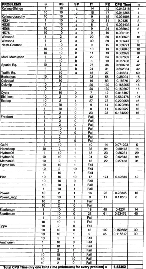
6 C O M P U T A T I O N A L R E S U L T S 61 6.1 Test P roblem s... 61

6.2 Experiment 1: Uniform Reduction of u ... 64

6.3 Experiment 2; A Hybrid Reduction Scheme for

u

7 C O N C L U S I O N 76 A U s e r ’ s G u id e to N C P N M S 8 6 A .l P u r p o s e ... 86

A .2 Specification of the Subroutine N C P N M S ... 86

A.3 Description of P a r a m e te r s... 87

A .4 U M F P A C K 2 ... 90

A.5 BLAS 91 A .6 Harwell R o u t in e s ... 91

6.1 Interior Plus-Smooth Function, CPU Time versus n

69

6.2 Piecewise Quadratic Plus-Smooth Function, CPU Time versus n 70

6..3 Piecewise Quadratic Plus-Smooth Function with Reduced Matrix 71

6.4 Comparison For CPU T i m e ... 72

6.5 Comparisons For CPU Time Per I t e r a t io n ... 73

6.1 Interior Plus-Smooth Function... 66

6.2 Piecewise Quadratic Plus-Smooth Function... 67

6.3 Piecewise Quadratic Plus-Smooth Function with Reduced Jaco­ bian M a t r i x ... 68

6.4 Hybrid Reduction S c h e m e ... 75

IN T R O D U C T IO N

Complementarity problems are important areas of applied mathematics due to their numerous applications: The complementarity theory derives its importance from the fact it unifies problems in fields such as: mathematical programming, game theory, the theory of equilibrium in a competitive economy, equilibrium of traffic flows, mechanics, engineering, lubricant evaporation in the cavity of a cylindrical bearing, elasticity theory, fluid flow through a semiimpermeable membrane, maximizing oil production, computation of fixed point etc.

Any mathematical programming model can be modeled as complementarity problem. Complementarity problem has been of great interest in the academic and professional communities ever since the path-breaking paper by Lemke and Howson. Especially after continuation methods and smoothing approaches complementarity problems became a very important subject. Because by using continuation methods and smoothing approaches, complementarity problems can be solved in computationally efficient time.

In this study, a continuation method for nonlinear complementarity problems via normal maps which was developed by Chen, Barker and Pinar [8]

is implemented. A software which is based on this algorithm is developed in ANSI FO R T R A N 77 to solve numerous complementarity problems, and the software package uses a sparse linear system solver UM FPACK2.

The organization of the thesis is as follows. In the next chapter definitions of nonlinear complementarity problem (NCP) and a summary of the most well known algorithms to solve NCPs are given. Then the smoothing method approximation and application of smoothing method for NCPs are explained in the third chapter. The fourth chapter consists of subproblems of Newton corrector we study. Numerical example is in the fifth chapter, explanation of algorithm is in the chapter six and numerical testing and comparison is in the chapter seven. The thesis concludes with some remarks and suggestions for future research.

The following notation will be used throughout the thesis. All matrices are denoted by boldface l e t t e r s . R " , d e n o t e , respectively,

n

LITER ATU R E R E V IE W

2.1

Overview

In this section, Nonlinear Complementarity Problems (NCP) are defined mathematically and the related literature is briefly reviewed. To begin, let us define the problem under investigation:

D efin itio n 2.1

Let F be a mapping from

to itself.

The nonlinear

complementarity problem (NCP), denoted by NCP(F) is to find a vector x

such that:

a; > 0,

F{ x) >

and F{x)^x

The first two inequalities are called the feasibility conditions, and the equality is called the complementarity condition.

When

F

D efin itio n 2 .2

Let

and q £ BT. The LCP is to find an x

such that:

The following definitions of various special matrices and functions will be used in subsequent chapters.

D efin itio n 2 .3

The matrix

is said to be a

1. Po-matrix if for all x ^ 0, there exists an index i such that Xi ^ 0 and

Xi(M x)i > 0,

2

. copositive matrix if

for all x >

0

,

3. copositive-plus matrix if it is a copositive matrix and for all x ^ 0, if

x ^ M x = 0,

then

4- positive semi-definite matrix if x^lS/ix >

for all x,

5. P-matrix if for all x ^ 0 , there exists an index i such that

6

. positive definite matrix if

for all x ^

0

,

7.

Ro-matrix if the following system has no solution:

X >0,

M i.x = 0 if Xi > 0, M j.x > 0 if Xi = 0,

8

. Q-matrix if LCP(M.^ci) has a solution for all q,

9. Z-matrix if mij <

for all i ^ j .

Among the above special matrices, the following relations hold: positive definite matrix P-matrix /o-m atrix;

positive definite matrix

=>

=>

D efin ition 2 .4

The mapping

is said to be a

1

. Po-function over a set X if

max

[Fi{x) - Fi{y)]'^{xi - y i ) > 0 \/,y e X ,x ^ y,

2

.P-function over a set X if

max[Pi(rc) - Fi{y)]'^{xi - yi) > 0 Vx, ?/ G X, x 7^ y,

3. uniform P-function over a set X if there exists an a > 0 such that

m&x[Fi(x) - Fi{y)]'^(xi - yi) >

ajja; -

y f Vx,y

€ X,

l<2<n

4

. monotone function over a set X if

[ F ( x ) - F ( y ) f ( x - y ) > 0 V x , y € X ,

5. strictly monotone function over a set X if

[F(x) - F { y ) f { x - y ) > O V x , y e X , x ^ y ,

6. strongly monotone function over a set X if

[F(a;) -

F { y ) f { x - y) >

y f Vx,y e X.

For the above definitions, the following relationships hold: Strong monotonicity strict monotonicity ^ monotonicity, Uniform P-property

=>

Strong monotonicity => uniform P-property, Strict monotonicity ^ P-property,

Monotonicity Po-property [4].

Let us now consider some examples which lead to complementarity problems.

2.2

Mathematical Programming

In this section we consider several examples and models in finite dimensional spaces. Hence we consider the topological vector space P " ordered by the pointed closed convex cone

RJf

2.2.1

Linear Programming

Let c =

(ci)

BA,b =

RP'

Consider the primal linear program,

minimize

< c ,x >

(P.L.P.)

x e F i

where, Fi = {a; G

R^

and its dual.

(D.L.P.)

maximize

< y,b >

y €: F

2

where,

F

2

= {y e

A fundamental result of linear programming is the following.

T h e o re m 2.1

If there exist X

F\ and yo

F

2

such that < c,Xo > —<

yo,b > then Xo is a solution of problem (P.L.P.) and yo is a solution of problem

(D.L.P.).

Using this result we can associate to the problem, (P.L.P.) and (D.L.P.) a complementarity problem.

Indeed, adding slack variables u G R " and u G i? " such that, A — v = b and A V + u = c and denoting. 2: =

y

w

u

_q

c

- b

0 - A

following complementarity problem.

Finder G i?”''’™such that

[L.C.P

We observe that this linear complementarity problem is equivalent to the couple primal-dual of linear programs (P.L.P.) - (D.L.P.).

Remarks:

i- ) Condition

< z,w > =

y, b >.

ii- ) The principal contribution of complementarity problem to the linear programming is that it transforms an optimization problem in an equation.

2.2.2

Quadratic Programming

Consider the quadratic programming problem,

(

1

)

f { x )

X ^ F

F = {x E R7\.-,b —

f { x )

c

Denoting the Langrangian multiplier vectors of the constraints A x < b and a; > 0 by A

G

G

u G

(

)

u

R ^ ,

< u, x > =

✓ u V (3) : < u V c +

Q

0

e RT^^·,

Rl+"^;<

u

u

we obtain that the Kuhn-Tucker conditions (2) are equivalent to the following linear complementarity problem,

find 2 G such that,

; G

RŸ"^-Jiz)

R Ÿ ”^

z , f { z )

( 4 ) : ^ +

It is remarquable to note that there exists another connection between linear programming, quadratic programming and the linear complementarity problem.

Consider the linear programming problem.

( 5 ) :

Minimize

< p, x >

X e F

where:

F

₌

{x

_Ç.

i?” |Ax — b G R“ }

^ p G R ” , 6 G R*" and

G Mn».n(R)

Suppose that every row of A is different from zero and consider a quadratic perturbation on F of problem (5) of the form.

(6_{) :} Minimize

[< p, x >

x e F

T h e o r e m 2 .2

If program (5) has an optimal solution then program (

6

) has a

unique solution

for every e

and some

Moreover, the solution

is independent of e and it is also a solution of program

(5).

Consider now a more general case, precisely the quadratic program,

( 7 ) d

Minimize [| < a;,Q x > + < p, x >] X

e F

where;

F = {x ^

p

G

b

G

K^',

G

G Mm*n(R)

The dual program of (7) is.

Maximize [—| < a;,

Qx

(x,u)

where:

Fi —

Rif:

which under the positive definite assumption on Q is, (upon eliminating x, since from (8)

x

Minimize (| <

u,

u e F

2

where: F2 = {u G

R^\u

Since A Q - ' A ‘ is positive semidefinite, (9) is equivalent to the following symmetric linear complementarity problem.

(S.L.C.P.)

Find

u

G R'" such that,

u

G

Rf\ V =

G R™ and < u,

2.2.3

Nonlinear Programming

Consider the convex program,

Minimize

f ( x )

(10) : ^ a: G F

where:

F = {x G R^lx

gi{x)

In this programming problem suppose all the functions convex and differentiable. The Lagrangian function

L{x,u)

m

L{x, u) = f { x ) +

Uigi{x).

i=l

Hence,

u

{ui)

BF

n

(11) d

- 2 ^ = A „ , . i ( x , « ) > 0 ; i =

_dui

l,2...,

m

a; > 0, u > 0

E "= i

Xjhj{x,u)

hi{x)

If we denote, ^ =

X

u

h[z) —

hji{x^

hn-\-m

then the Kuhn-Tucker conditions (11) may be stated as the following complementarity problem.

(C. R) :

find ₂:

E

2T €

h(z) E

<

2

;,

h(z) > —

Remark:

We have a similar construction for a nonlinear program (not necessarily convex), where / and

gi(i

U,

such that

U

R^.

2.3

The Homotopy Principle

Suppose that a system of nonlinear equations is given for you to solve. Our immediate goal is to find a point x = ( x i , ..., Xn) that solves such a system. How might we accomplish this? One approach is to start with another system of equations to which we already know the solution. Usually, this is a particularly simple system that has an obvious solution. We then take this simple system and mathematically ’’ bend” it into the original system. While bending the system we carefully watch the solution, as it also ’’ bends” from the obvious solution into the solution we seek. This bending notion underlies a key idea that we shall develop shortly, the

homotopy

Let i?" denote

Euclidean n space.

F : RT ^ BA

F{ x)

has n components,

F{ x)

(Fi(a;),

F„(a;)),

x

X

= ( x i , ..., ,T„),

Fi{F^

I

We are desirous of solving the

n x n

(x) = 0

First set up a simple system

Then define a special function, called a

homotopy function, H{ x, i )

i?”,

n

t.

(x,t)

=

(xi, ...,Xn,t) E

H

H{x, 0) = E{x)

H{ x , l ) = F{ x)

It follows that at t = 0,

H(x,0) =

has a solution which we already know, and at t = 1,

H{ x , l ) = 0

has solution

x*,

t, x{t)

H{x{t), t) —

The idea is to start at a;(0) = and then increase

t

x(t)

2.3.1

Varieties of Homotopies

Newton Homotopy

H{ x, t) = F{ x) - {1 - t)F{x^).

This form of homotopy is termed the

Newton homotopy

x^.

F{x°),

E{x) = F{ x) - F(x°).

The function

E,

selected arbitrarily, the Newton homotopy permits us to start the path from wherever we choose, a very nice feature.

Fixed-Point Homotopy

H(x, t) =

(1

— t)(x —

tF{x).

This homotopy, called the

fix ed — point homotopy.

E{x) = X — x° =

0

so that o:(0) = The fixed-point homotopy is thus also easy to start since

x^

can be chosen arbitrarily.

Both the fixed-point and Newton homotopies can be started from any point which is one of the reasons that both are so widely employed.

The homotopy approach has been known to scientists at least since the nineteenth century. It is a standard tool in the theory of ordinary differential equations (Ficken [1951]). The first application to nonlinear equation systems seems to have been made by Lahaye [1948]. The first fail-safe general procedure for fixed point and related equation systems is due to Scarf [1967]. In actuality. Scarf did not use a homotopy approach but an entirely novel approach which he called primitive sets. An earlier work related to Scarf’s fundamental work is Cohen [1967]. The underlying principle used by Scarf to prove convergence of his procedure is the ’’ complementarity principle” of Lemke and Howson [1964].

2.4

Lemke’s Algorithm

Lemke’s algorithm is designed to solve the LCP. Given

q

d E R^

z — d + q T

Clearly this equation has a trivial solution a; = 0, where

z = d + q.

Hi{x, t) —

Zi}

i =

,

n

iov z

t)d + q +

z^x

z >

0

2 = (1 —

t)d

At t = 0, notice that the trivial LC with trivial solution x = 0 is obtained, whereas when i = 1, we have the original LC.

Lemke’s method traces the path in

H~^

Hi{x,t) = mm{xi,Zi} =

0

,

i =

where

■2 — (l — /)d T 9 T

AIx

To avoid degeneracies a regularity condition is required: For each ( x ,i) €

H~^,

at least n — 1 of the variables x,z are greater than zero.

Algorithm

Step

Initially, = (0 ,0 ),

=

t

z + td = d + q

z >

0

,

t ^ R}

1. If

t

Zi

t — P.

=

Let

(x^,P)

wi

=

(ui,

...Un)

ui = ... — Un = 0.

wi

A*'w + td = d + q

tu > 0,

t E R}

where A f = e* and

Wi

Zi.

1. If i becomes equal to 1, terminate. We have an LC solution at hand.

2. If

wt

3. Otherwise, some

Wj

wt = wt >

u>i = wi,

Wj

=

k +

1

.

Repeat this process until i = 1 or the path diverges to infinity.

Lemke’a algorithm historically form the basis for path-following procedures. The LC homotopy is not differentiable but does have a special structure which by use of Lemke’s algorithm produces a piecewise-linear path [18].

I divided solution methods and algorithms for NCP into four classes; non- differentiable equation approach, continuation methods, smoothing methods and non-interior continuation methods for review. However, these classes are not strictly independent. Non-interior continuation methods consists of smoothing methods and continuation methods, also smoothing methods consists of continuation methods, etc... Now let’s look at some algorithms which were developed after Lemke’s algorithm for NCP. Firstly, we give make some definitions.

D efin itio n 2 .5

If a method maintains strictly feasible (x^ >

0

or F{x)'^ >

(strictly greater than zero) for every iteration of solution procedure of NCP,

then method can be called interior method. Otherwise, it is called a non-interior

method.

A lot of solution approaches exist for solving the N C P (F ). Kostreva [21, 37, 38] developed a block-pivoting algorithm in which multiple exchanges of basic and nonbasic variables are executed. This algorithm extended Murty’s scheme [50] for TC P’s to the nonlinear complementarity setting. This method must solve a system of nonlinear equations at each iteration, and does not contain a line search step.

Subramanian [64] used a Gauss-Newton method to solve the nonlinear complementarity problem when formulated as the continuously differentiable equation system first introduced by Mangasarian [42]. While deriving some convergence results, no extensive computational evidence was reported.

Kojima, Mizuno, Nome and Yoshise [36, 35, 34, 33] have developed interior- point algorithms for solving monotone linear and nonlinear complementarity problems. When the matrix is positive semi-definite in the linear case, they show that the complexity of their algorithm is polynomially bounded; some limited computational results for this case were also reported. For the nonlinear case, the convergence theory exists for uniform P-functions, but only limited convergence results exist when

F

In addition to these methods, non-interior continuation methods also were developed. Non-interior continuation methods are closely related to path­ following interior point algorithms. Non-interior continuation methods take a different deformation of the complementarity condition. As a result, they did not have to restrict intermediate iterates to stay interior (detailed inforrnation can be found in section 2.8).

2.5

Non-differentiable Equation Approach

A successful algorithm for the general NCP is the Josephy-Newton [27, 28] method which is based on Robinson’s generalized equation approach for analyzing problems such as the NCP. The basic idea is to linearize the function

F( x)

x^,

x^'^^

F(x^)

VF(x^)( x

The quadratic convergence rate of Newton’s method is one of the most important features of this approach. However, the convergence theory for this method requires that one start close to the solution x*. To overcome this problem, Mathiesen [46, 47] and Preckel [57] have introduced various heuristic line search procedures to widen the region of convergence.

The N C P (F ) can easily be formulated as a system of nonlinear equations as follows:

H(x) = mm(x, F( x) )

where the ” min” operator is taken component-wise. While this system of equations is simple, it is not differentiable [54] and thus, the traditional Newton method does not apply. It is, however, B-differentiable. Robinson [59, 60, 61, 62] first studied B-differentiable functions and Newton’s method for a class of such nonsmooth functions. Pang [55] presents a generalized Newton algorithm for the above system of B-differentiable equations which is globally convergent under certain assumptions. Harker and Pang [23] then used these results to develop a damped-Newton method for the linear complementarity problem, and showed through extensive computational experiments that this method is potentially very efficient as compared with Lemke’s method.

Harker and Xiao [24] extended the work by Harker and Pang to the nonlinear complementarity problem. Instead of using ” min” operator, Harker

and Xiao converted the nonlinear complementarity problem into a system of equations through the use of a Minty-map [36, 61, 62]. The algorithm presented was similar to Kostreva’s direct block pivotal algorithm, except that they solved a linear system of equations at each iteration and performed a line search to minimize a given merit function. This merit function minimization is what generates the global convergence properties of the algorithm in much the same way as in solving F-differentiable equations [29]. Minty-map formulation [36, 61, 62];

H{x)

E(x'^) A

where

x f

x~ =

x~ =

(x]·, x j , ...x “ )^. It is easy to verify that there is a one-to-one correspondence between a solution of N C P (F ) and a solution of the system of equations

H{x) - F(x'^)

In other words, x solves this equation if and only if x+ solves the N C P (F ). Hence, the nonlinear complementarity problem can be formulated as a system of nonlinear equations different from first Minty map formulation [24]. Marker and Xiao used B-differentiable functions in their algorithm [24].

D efin ition 2 .6

A function H ·. RA ^ BA is said to be B-differentiable at the

point

if H is Lipschitz continuous in a neighborhood of x and there exists a

positive homogeneous function

called the B-derivative of H

at

such that

,.

H {x + v ) ~ H { x ) - B J i ( x ) v

v-o ||v||

H is said to be B-diffei'entiable in a set X if H is B-differentiable at all points

X e X .

2.5.1

The Damped-Newton algorithm

The damped-Newton algorithm [24] which is used to solve the above equation system (minty-map formulation) is stated as follows. Let x° G be an arbitrary initial vector, let

s,p,

a

and (T G (0, |). In general, given with ||ff(a;^)|| > e > 0 where

e

Stepl.

E R^:

H{x'^)

Step

2

.

\k =

rrik

g{x'^) — g{x^^

g™'sd'^) >

2

apT^sg{x^).

where

g{x) — \H{x)^H[x) =

x^~^^ = x^

Xkd'^·

H(x^) < e.

Pang [55] derived local and global convergence results for the damped-Newton method applied to a system of B-differentiable equations.

Although this algorithm doesn’t use smoothing methods, its structure is similar to our algorithm [8]. Therefore it is included here to give a background to the readers.

2.6

Continuation Methods

Continuation methods study the relationship between a problem

P,

Pie)

P.

e

P.

P(e)

e

P

P{e).

Now, we will mention a continuation method which is developed by Kanzow [30]. This study is one of the recent studies and it is similar to previous Lemke’s algorithm and our algorithm. Therefore we thought that it is suitable to give Kanzow’s algorithm [30].

2.6.1

Interior-point continuation method for comple­

mentarity problems with uniform P-functions

This is based on [30]. Let /i > 0 be given. The main tool used in this method is the function

: R^

R

<p^(a, b) — a + b - \J {a- by

In the special case

p = 0, ipfj, = ipo

b) — a + b — sqrt{a — bY = a + b — \a — b\ —

The function m in{a,

b}

: R^"'

by

F {x ) - y

=

where

Kanzow stated a theorem saying that a vector

z{y)

{x{ii),y{ix))

F^p^{z) —

¡

1

)

(x{iJ,),y{iJ,))

R?^

a? > 0, ?/ > 0,

Xiyi = n, y = F {x) i =

If yu = 0 the problem P N C P (/, reduces to the nonlinear complementarity problem.

2.6.2

Kanzow’s algorithm:

StepO.

{pk}keN

Stepl.

Step

2

.

— z{p,k+i)

of the nonlinear system of equations

(^) = 0

StepZ.

k = k +

1

Stepl

2.7

Smoothing Methods

The complementary condition

0 <

xL y

where

x

y

BA

x

y

X = (x -

y)+

where the plus function (.)+ is defined as

(£)+ = m ax{£, 0 },

for a real number

e.

employed.

Smoothing techniques have already been applied to different problems, such as, /j-minimization problems [41], multi-commodity flow problems [56], nonsmooth programming [68, 39], linear and convex ineqaulities [10], and linear complementarity problems [5], [10] and [30]. These successful techniques motivate a systematic study of the smooth approach.

2.7.1

A class of smoothing functions

In this section we review a class of smooth approximations to the fundamental function (a;)+ = m ax{a;,0} [11]. Notice first that =

f^^cr{y)dy,

a{x)

r(a;) = 1 if X > 0 0 if X < 0

The step function <t(x) can in turn be written as, cr(x) =

S(y)dy,

r+oo

/

S{y)dy

-oo

The fact that the plus function is obtained by twice integrating the Dirac delta function, prompts us to propose probability density functions as a means of smoothing the Dirac delta function and its integrals. Chen and Mangasarian [11] considered the ¡jiecewise continuous function

d(x)

/

d{x)dx

To parametrize the density function Chen and Mangasarian defined

where

/3 is a,

^

t[x,(3)

6

{x).

follows:

and

i(x,/3)= I

i{t, ^)dt ^ a{x)

J — CO

P (x,l^ )= I

s{t,^)dt?=i {x)+

Therefore, Chen and Mangasarian got an approximate plus function by twice integrating a density function. In fact, this is the same as defining

I {x -t)i{t,l3 )d t.

Now, let’s look at some smooth plus function examples:

E x a m p le 2.1

Neural Networks Smooth Plus Function [10]: Let

d{x)-(1 +

e~^y

Here D\ —

2,

= 0 and suppd{x)

R, where

/•0

D i =

\x\d{x)dx

J

and

D

2

= max{

xd {x)d x,

0

}

J

Integrating a —

we have

p{x, a) = p{x,

a)d^

a

J

a

s(x, a)

s{x,

=

j

a)dC

1

t{x, a) = t{x,

ae

OL

E x a m p le 2 .2

Chen-Harker-Kanzow-Smale Smooth Plus Function [63], [30],

and [5]:

Let

d{x)

{x^

Here D\ = 1, D

2

=

supp{d{x)} = R and

E x a m p le 2 .3

Pinar-Zenios Smooth Plus Function [56]:

Let

'

1

i f O < t

< 1

otherwise

Here D\, D

2

=

supp{d{x)} =

and

d{x)

p{x,II) = <

0 e/a; < 0 2/3

i f O < x < P

X - ^

if X > jd

E x a m p le 2 .4

Zang Smooth Plus Function [

68

]:

let

d{x)

■

’

~ ~

[ 0

otherwise

Here Di

supp{d{x)} =

and

p{x,/3) =

0

i f x < - §

¿ ( a ; + 1)2

₂

_p

i / | a ; | < f

X

_{i f x > §}

2.7.2

Application to The Nonlinear Complementarity

Problem

Recall that NCP is the problem of finding an

x

0 < a;±F(a:) > 0

Here

F {x)

R^.

p[x,P )

R{x) = X — p(x — F {x), Id) = 0

is proposed as an approximation to the following nonsmooth equivalent reformulation of the NCP

And now we can specify Chen and Mangasarian’s algorithm [11]. The algorithm consists of a Newton method with an Armijo line search with parameters

6

cr

xo E

dk

dk

= -V R (xk )“ ^R(xk)

(2) S tep size A*; (Armijo)

X k + i = Xk + \ k d k , X k =

max{l,i,i^,

fi^k) - f{xk+i) >

k = k + I go to

The above algorithm is well defined for a monotone NCP with a continuously differentiable

F {x).

2.7.3

Mixed Complementarity Problem

The mixed complementarity problem (M CP) is defined as follows [15]: Given a differentiable F : i?" —> i?” ,

l,u E

■

, I <

R = R C

x ,w ,v ,E

F {x) — w A

— 0

0 <

iLw

vLu

This M CP model includes many classes of mathematical programming problems, such as nonlinear equations, nonlinear programming, nonlinear complementarity problems and variational inequalities.

By using the smooth function

p{x,/d)

i =

Case 1.

li

Ui —

Case 2. /j > —oo and

U{ =

Xi - k - p{xi - k - Fi{x),

li

Ui <

Xi — U i + p{ui - Xi + Fi{x),/3) — 0

Case 4.

h

ui <

Fi{x) -W i + Vi = 0

Xi - h — p{xi — k

.

Chen and Mangasarian denoted the above 4 cases collectively by the nonlinear equation

R(x, w ,v) = 0

Note that the natural residual for the MCP is given by the left hand side of above relation with the

p

Let

f { x ,w ,v )

f{ x ,w ,v )

- R { x ,w ,v Y R {x,w ,v)

C h en and M a n g a sa ria n ’ s S m o o th A lg o r ith m for M C P [1 1]: Input tolerance e, parameter

p > \

RA

(1) In itialization For 1

< i < n oi

W

=

V

a{xo,wo,vo).

amax -

(2) N e w to n A r m ijo S tep Find

(xk^i,Wk+i,Vk+i)

R {x,w ,v ) =

(3) P a ra m e te r U p d a te If

a{xk+i,Wk+i,Vk+i)

ucnk,

otherwise if ||Vf(xk+i, Wk+i,Vk+i)||2 < e, set

Oik+i = ^ock

2.8

Non-interior Continuation Methods for

the NCP

Finally, let’s look at non-interior continuation methods. Non-interior continuation methods are closely related to path-following interior point algorithms. Both methods deform the complementarity condition by a parameterized systems of smooth nonlinear equations, then solve the deformed NCP by Newton’s method approximately, and adjust the parameter to refine the deformation. Both feasible and infeasible interior point path following algorithms have been developed to solve linear complementarity problems (LCPs) and NCPs (see for example [48, 49, 52, 53, 65, 66]). Wright and Ralph [66] proposed to alternate between the Newton step for the NCP and the centering step for the deformed NCP to achieve global and local superlinear convergence. However, no global convergence rate was given for their algorithm. Tseng [65] took a different approach by choosing certain combination of the above two steps as a search direction at each iteration. For the first time, he showed both global linear convergence and local superlinear and quadratic convergence for monotone NCPs with some additional assumptions. All interior point algorithms, however, share a common feature: they require each intermediate iterates to stay interior (positive).

Non-interior continuation methods take a different deformation of the complementarity condition. As a result, they did not have to restrict intermediate iterates to stay interior. The first non-interior method was introduced by Chen and Marker [5], where the authors concentrated on establishing the structural properties of the central path for LCPs with Po and

Ro

[5, 30] compared with interior point algorithms. As a result, no rate of convergence results were obtained. This gap was closed recently by Burke and Xu [2]. Inspired by many path following interior point algorithms, the authors introduced a notion of neighborhood around the central path for their non-interior continuation methods. All intermediate iterates are required to stay within the neighborhood and this provides a systematic procedure to reduce the smooth parameter. This important addition to the continuation methods allowed them to establish the global linear convergence for both LCPs with Po and

Ro

P

All non-interior continuation methods mentioned above are based on smooth functions derived from

XiPi

fx,

The non-interior continuation methods are also closely related to a broader class of algorithms called smoothing methods, which have attracted much attention recently. In particular, Gabriel and Moré further generalized the Chen-Mangasarian smooth function family and applied their smooth functions to mixed complementarity problems [17]. Chen, Qi and Sun [13] designed a smooth Newton method to solve a system of non-smooth equations and showed global and locally superlinear convergence for their method. Their results are based on a even broader class of smooth functions than the Gabriel- More family. The method was then applied to solve general box constrained variational inequalities. More recently, Chen [12] developed a smoothing quasi-Newton method for non-smooth equations and established superlinear convergence for the algorithm.

2.8.1

A Continuation Method for N C P

A recent contribution was made by Chen and Xiu [9], which gave a globally linearly and locally quadratically convergent algorithm. This recent non­ interior method is conceptually important and therefore we put it here. Recall that NCP can be written as:

min{a;, y} = 0 or a; — (a; —

y)+

where the plus function is taken component-wise. By deforming the plus function with the Chen-Mangasarian smooth function

p^,

= X - Pn{x - y ) =

0

,

where > 0 is a smooth parameter,

P^{x — y)

'^nix^y) =vec{xj;^{xi,yi)}.

The smoothed NCP then becomes:

Hf,{x,y) -

F {x) - y

'^^^{χ,y)

= 0,

and the NCP conditions (l)-(2 ) can be written as

H o{x,y)

H ^{x,y)

p, >

0

p

p

Chen and Xiu [9] mentioned importance of the structure of the Jacobian matrix for the convergence analysis:

Denote

P'fi{z) =dia.g{p[Xzi)}.

and

^ - y) =

K ( y

P'^(y - x ) <

1

.

Thus, the Jacobian matrix can be written as

V H ,(x ,y ) =

V F (x )

- I

.

K ( y -

K (^ - y)

It is well known that the Jacobian

^(x^y),

P'^{y

P^(x — y){x)

Hfj,{x,y):

Pf^i^^y) =

Let the central path(s) of the NCP be the set of solutions of

Hf^{x,y) =

^il^)

where parameter ^ > 0 is called the width of the neighborhood. In addition, they defined the slice of neighborhood with /x G 17 as

=

pf,{x,y)

For simplicity, if 17 = /x, they wrote the slice as

C h en and X i u ’ s C on tin u a tio n A lg o r ith m [9]: Given

cr

ai

S tep 0 (Initialization)

Set

k = 0.

po >

/3 > nB

N{/3,po).

S tep 1 (Calculate Centering Step)

If

Ho{x'^, y^) =

y^)

y^)

is singular, stop. The continuation method fails; otherwise, let (A x *, A y*) solve the equation