SOLUTIONS OF LARGE-SCALE ELECTROMAGNETICS PROBLEMS USING AN ITERATIVE INNER-OUTER
SCHEME WITH ORDINARY AND APPROXIMATE
MULTILEVEL FAST MULTIPOLE ALGORITHMS ¨
O. Erg¨ul, T. Malas, and L. G¨urel †
Computational Electromagnetics Research Center (BiLCEM) Bilkent University
Ankara, Turkey
Abstract—We present an iterative inner-outer scheme for the efficient solution of large-scale electromagnetics problems involving perfectly-conducting objects formulated with surface integral equations. Problems are solved by employing the multilevel fast multipole algorithm (MLFMA) on parallel computer systems. In order to construct a robust preconditioner, we develop an approximate MLFMA (AMLFMA) by systematically increasing the efficiency of the ordinary MLFMA. Using a flexible outer solver, iterative MLFMA solutions are accelerated via an inner iterative solver, employing AMLFMA and serving as a preconditioner to the outer solver. The resulting implementation is tested on various electromagnetics problems involving both open and closed conductors. We show that the processing time decreases significantly using the proposed method, compared to the solutions obtained with conventional preconditioners in the literature.
1. INTRODUCTION
For numerical solutions of electromagnetics problems involving metallic (conducting) objects, simultaneous discretizations of surfaces and the integral-equation formulations lead to N × N dense matrix equations,
Received 17 June 2010, Accepted 2 July 2010, Scheduled 22 July 2010
Corresponding author: ¨O. Erg¨ul ([email protected]).
† O. Erg¨¨ ul is now with the Department of Mathematics and Statistics, University of Strathclyde, Glasgow, UK; T. Malas is now with the Department of Electrical and Computer Engineering, The University of Texas at Austin, Austin, Texas; L. G¨urel is also with the Department of Electrical and Electronics Engineering, Bilkent University, Ankara, Turkey.
which can be solved iteratively by using a Krylov subspace algorithm. On the other hand, most of the real-life applications involve large geometries that need to be discretized with millions of unknowns. For such large-scale problems, it is necessary to reduce the complexity of the matrix-vector multiplications required by an iterative solver. The required acceleration is provided by the multilevel fast multipole algorithm (MLFMA), which is based on calculating the interactions between the discretization elements in a group-by-group manner [1]. This is achieved by applying the addition theorem to factorize the free-space Green’s function and performing a diagonalization to expand the spherical wave functions in a series of plane waves [2]. Constructing a tree structure of clusters‡ by recursively dividing a computational box enclosing the object, MLFMA computes the interactions in a multilevel scheme and reduces the processing time of a dense matrix-vector multiplication from O(N2) to O(N log N ). In addition, only a
sparse part of the full matrix, namely, the near-field matrix, needs to be stored so that the memory requirement is also reduced to O(N log N ). Consequently, MLFMA renders the solution of large matrix equations possible on relatively inexpensive computing platforms.
MLFMA offers remarkable advantages for the iterative solution of integral-equation formulations by reducing the complexity of the matrix-vector multiplications [3, 4]. However, particularly for large-scale problems, it is desirable to further reduce the total cost of the iterative solutions. For example, Bouras and Frayss´e [5] proposed decreasing the accuracy of the matrix-vector multiplications in the jth iteration by relating the relative error δj of the matrix-vector
multiplication to the norm of the residual vector ρj, i.e.,
δj = ε, kρjk2> 1 ε kρjk2, ε ≤ kρjk2 ≤ 1 1, kρjk2< ε, (1)
where ε ≤ 1 denotes the target residual error. Using (1), the relative error of the matrix-vector multiplication is relaxed from ε to 1 as the iterations proceed. However, using a similar relaxation strategy by adjusting the accuracy of MLFMA during the course of an iterative solution is not trivial. This is because the implementation details of MLFMA depend on the targeted accuracy. In principle, it is possible to construct a fixed number of MLFMA versions with various levels of accuracy. Nevertheless, each version increases the cost of the setup substantially. Moreover, a less-accurate MLFMA obtained by ‡ Throughout this paper, the term “clusters” is used to indicate “boxes” and “sub-boxes” in an MLFMA oct-tree.
decreasing the number of accurate digits is not significantly cheaper than the ordinary MLFMA.
Another option for reducing the cost of an iterative solution is to use preconditioners to accelerate the iterative convergence. In MLFMA, the sparse near-field matrix is available to construct effective preconditioners for relatively small problems. However, as the problem size grows, sparsity of the near-field matrix increases, and the resulting preconditioners become insufficient to accelerate the iterative convergence.
In this paper, we present efficient solutions of large-scale electromagnetics problems using ordinary and approximate versions of MLFMA in an inner-outer scheme [6, 7]. Outer iterative solutions are performed by using a flexible solver accelerated by an ordinary MLFMA. Those solutions are effectively preconditioned by another Krylov-subspace algorithm accelerated by an approximate MLFMA (AMLFMA). There are two explanations to describe the advantages of the proposed strategy:
(i) Matrix-vector products performed by an ordinary MLFMA are replaced with more efficient multiplications performed by AMLFMA. Different from the relaxation strategies, however, only a single specific implementation of AMLFMA is sufficient to construct an inner-outer scheme. In addition, a reasonable accuracy (without strict limits) is sufficient for the approximation. (ii) Iterative solutions by an ordinary MLFMA are preconditioned with a very strong preconditioner that is constructed by approximating the full matrix instead of the sparse part of the matrix.
In this paper, AMLFMA is introduced and proposed as a tool to construct effective preconditioners. We consider the iterative solutions of large-scale electromagnetics problems and demonstrate the acceleration provided by the proposed strategy based on AMLFMA, compared to the conventional preconditioners.
The rest of the paper is organized as follows. Section 2 outlines efficient solutions of surface formulations via MLFMA. In Section 3, we discuss various techniques to construct less-accurate versions of MLFMA, and point out the advantages of the proposed AMLFMA scheme. Sections 4 and 5 present examples of conventional near-field preconditioners and some details of the proposed preconditioning technique based on AMLFMA, respectively. Then, we provide numerical examples in Section 6, followed by our conclusion in Section 7.
2. SOLUTIONS OF SURFACE INTEGRAL EQUATIONS VIA MLFMA
Using MLFMA, matrix-vector multiplications required by the iterative solvers are performed as
Z · x = ZNF · x + ZF F · x, (2)
where only the near-field interactions denoted by ZN F are calculated directly and stored in memory, while the far-field interactions denoted by ZF F are calculated approximately and efficiently [8]. Consider a metallic object of size D discretized with low-order basis functions, such as the Rao-Wilton-Glisson (RWG) [9] functions on λ/10 triangles, where λ = 2π/k is the wavelength. For smooth objects, the number of unknowns is N = O(k2D2). A tree structure of L + 2 = O(log N )
levels is constructed by recursively dividing the object until the box size is about 0.25λ. We note that the highest two levels are not used explicitly in MLFMA, and the number of active levels is L. At each level l from 1 to L, the number of clusters is Nl, where N1 = O(N )
and NL = O(1). To calculate the interactions between the clusters,
radiation and receiving patterns are defined and sampled at O(Tl2) angular points, where Tl is the truncation number. For a cluster of size al = 2l−3λ at level l, the truncation number is determined by
using the excess bandwidth formula [10] for the worst-case scenario and the one-box-buffer scheme [11], i.e.,
Tl≈ 1.73kal+ 2.16(d0)2/3(kal)1/3, (3)
where d0 is the desired digits of accuracy. We note that Tmin = T1=
j
2.72 + 2.51d2/30 k
+ 1 (4)
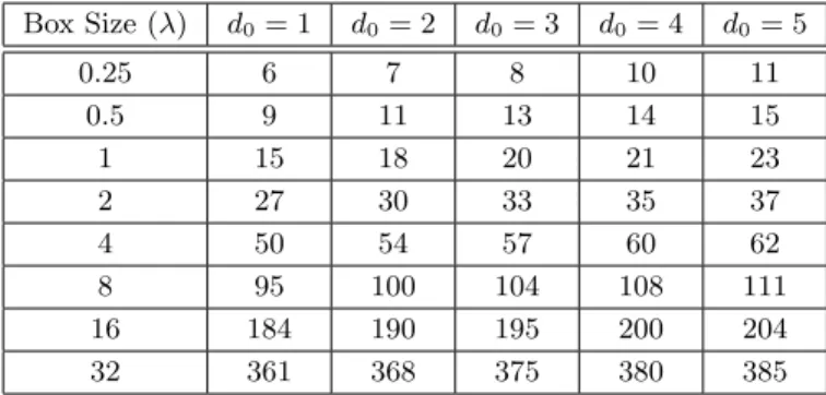
for the lowest level (l = 1) with a = 0.25λ, where b·c represents the floor operation. Table 1 presents a list of truncation numbers for different box sizes and when the number of accurate digits varies from d0 = 1 to d0 = 5. In general, the truncation number grows rapidly
as a function of the cluster size. In fact, for a large-scale problem, Tmax= TL= O(kD) and the maximum truncation number is linearly
proportional to the electrical size of the object. We also note that the truncation number loosely depends on the value of d0 for large
clusters [12].
2.1. Setup of MLFMA
Table 1. Truncation numbers (Tl) determined by the excess
bandwidth formula for the worst-case scenario and the one-box-buffer scheme. Box Size (λ) d0= 1 d0= 2 d0= 3 d0= 4 d0= 5 0.25 6 7 8 10 11 0.5 9 11 13 14 15 1 15 18 20 21 23 2 27 30 33 35 37 4 50 54 57 60 62 8 95 100 104 108 111 16 184 190 195 200 204 32 361 368 375 380 385
Input and Clustering: In the input and clustering stage, the discretized object is read from a file and a tree structure is constructed in O(N ) time. The amount of memory required to store the data is also O(N ).
Near-Field Interactions and the Right-Hand-Side (RHS) Vector: Near-field interactions and the elements of the RHS vector are calculated. Both the processing time for those calculations and the memory required to store the data are O(N ). Radiation and Receiving Patterns of the Basis and Testing Functions: Since they are used multiple times during the iterative solution part, radiation and receiving patterns of the basis and testing functions are calculated and stored in memory. These patterns are evaluated with respect to the centers of the smallest clusters, and O(T2
min) samples are required for each basis
and testing function. Then, the complexity of the radiation and receiving patterns is O(N T2
min) = O(N ), since Tminis independent
of N .
Translation Functions: Translations are performed between pairs of distant clusters, if their parent clusters are close to each other. Using cubic (identical) clusters, the number of translation operators can be reduced to O(1), which is independent of N , using the symmetry at each level. Consequently, for level l, O(T2
l)
memory is required to store the translation operators. On the other hand, direct calculation of those operators requires O(T3
l)
time, which is significant for the higher levels of the tree structure. Specifically, at the highest level with TL= O(kD) = O(N1/2), the
processing time required to evaluate the translation operators is O(N3/2). Due to this relatively high complexity, calculating the
translation operators results in a bottleneck when the problem size is large. As a remedy, local interpolation methods can be used to reduce the complexity to O(N ) without decreasing the accuracy of the results [12].
2.2. Matrix-vector Multiplications via MLFMA
During an iterative solution, each matrix-vector multiplication involves the following stages.
Near-Field Interactions: Near-field interactions that are stored in memory are used to compute the partial matrix-vector multiplications ZN F · x in O(N ) time.
Aggregation: In the aggregation stage, radiated fields of clusters are calculated from the bottom of the tree structure to the highest level. At the lowest level, radiation patterns of the basis functions are combined in O(N T2
min) time. Then, the radiated fields of the
clusters in the higher levels are obtained by combining the radiated fields of the clusters in the lower levels. Between two consecutive levels, interpolations are employed to match the different sampling rates of the fields. Using a local interpolation method, such as the Lagrange interpolation, aggregation operations for level l are performed in O(NlTl2) time [8]. The amount of memory required
to store the radiated fields is also O(NlTl2).
Translation: In the translation stage, radiated fields of clusters are converted into incoming fields for other clusters. For a cluster at any level, there are O(1) clusters to translate the radiated field to. Since the radiated and incoming fields are sampled at O(T2
l) points, the total amount of the translated data at level l is
O(NlTl2).
Disaggregation: In the disaggregation stage, total incoming fields at cluster centers are calculated. The total incoming field for a cluster is the combination of the incoming fields due to translations and the incoming field from its parent cluster. The incoming field to the center of a cluster is shifted to the centers of its subclusters by using transpose interpolations (anterpolations) [13]. Finally, at the lowest level, incoming fields are received by the testing functions via angular integrations. The complexity of the disaggregation stage is the same as the complexity of the aggregation stage, i.e., O(NlTl2).
In MLFMA, complexities of both processing time and memory are O(NlT2
l ) for level l. At the lowest level, T1 = Tmin = O(1),
O(N1/2), N
L= O(1), and O(NLTL2) = O(N ). In fact, considering the
numbers of clusters and samples, the complexity remains the same as O(N ) for each level. Thus, the overall complexity of a matrix-vector multiplication is O(N log N ).
3. STRATEGIES FOR BUILDING A LESS-ACCURATE MLFMA
MLFMA can perform a matrix-vector multiplication with a specific level of accuracy, which is controlled by the excess bandwidth formula in (3). There are many studies that further improve the reliability of the implementations by refining formulas for the truncation numbers, especially for small clusters [11]. In most cases, the purpose is to obtain accurate results by suppressing the error sources in MLFMA. On the other hand, it is also desirable to build less-accurate forms of MLFMA, which can be more efficient than the original MLFMA. A less-accurate MLFMA can be used to construct a strong preconditioner, where the accuracy is not critical, but a reasonable approximation with high efficiency is required.
A direct way to construct a less-accurate MLFMA is to reduce the truncation numbers using (3). For example, if the ordinary MLFMA has four digits of accuracy, i.e., d0 = 4, then a less-accurate MLFMA
may have one or two digits of accuracy [14]. This strategy, however, has two major disadvantages:
(i) A less-accurate MLFMA obtained by decreasing d0 in (3) is not significantly faster than the ordinary MLFMA, because, as listed in Table 1, the truncation number loosely depends on d0 for large
boxes at the higher levels of MLFMA. As an example, let d0 be
reduced from 4 to 1. At the lowest level involving 0.25λ boxes, the truncation number drops significantly by 40% (from 10 to 6). On the other hand, for a higher level with 16λ boxes, the truncation number decreases from 200 to 184, which corresponds to a mere 8% reduction. Therefore, reducing the value of d0does not provide
a significant acceleration, especially when the problem size is large. (ii) The extra cost of a less-accurate MLFMA obtained by decreasing d0 can be significant due to the calculation of the radiation and
receiving patterns of the basis and testing functions during the setup stage. In addition to the ordinary patterns employed by the ordinary MLFMA, a new set of patterns is required for the less-accurate MLFMA with the reduced truncation numbers. Because of the above drawbacks, better strategies are required to construct less-accurate yet efficient versions of MLFMA.
Another strategy to build a less-accurate MLFMA is by omitting some of the far-field interactions. In this case, the number of accurate digits is the same as that for the ordinary MLFMA, but the aggregation, translation, and disaggregation stages are omitted for a number of the higher levels of the tree structure. The resulting less-accurate MLFMA is called the incomplete MLFMA (IMLFMA), which does not require extra computations during the setup stage. In addition, IMLFMA can easily be obtained via minor modifications to the ordinary MLFMA. However, this strategy fails to provide an acceptable accuracy with a sufficient speedup. For example, half of the levels must be ignored to obtain a two-fold speedup with IMLFMA compared to the ordinary MLFMA; this leads to a poor approximation since it results in most of the interactions (much more than 50%) being ignored.
In this paper, we propose AMLFMA, which is based on systematically reducing the truncation numbers, i.e.,
Tlr= Tmin+ af(Tl− Tmin), (5)
where Tmin is the minimum truncation number defined in (4) and Tl
is the ordinary truncation number for level l. In (5), af represents an
approximation factor in the range from 0.0 to 1.0. As af is increased
from 0.0 to 1.0, AMLFMA becomes more accurate but less efficient, and it corresponds to the ordinary MLFMA when af = 1.0. Since the truncation number at the lowest level is not modified, AMLFMA does not require extra computations for the radiation and receiving patterns of the basis and testing functions. Only a new set of translation functions is required, which leads to a negligible extra cost.
As an example, we consider the solution of electromagnetics problems involving a sphere of radius 6λ and a 20λ × 20λ patch, discretized with 132,003 and 137,792 unknowns, respectively. For both problems, matrix-vector multiplications are performed by AMLFMA with various values of af. In addition to AMLFMA, we also consider
IMLFMA, which is constructed by omitting the interactions at only the highest level. The number of active levels (L) is five and six for the sphere and patch problems, respectively. The input array is filled with ones, and the output arrays provided by AMLFMA and IMLFMA are compared with a reference array provided by the ordinary MLFMA with three digits of accuracy. For each element of the output vector m = 1, 2, . . . , N , a base error is defined as
∆b[m] = dlog10(∆r[m])e, (6)
where d·e denotes the ceiling operation and ∆r[m] represents the
relative error with respect to the reference value provided by the ordinary MLFMA.
0 5 10 15x 10 4 AMLFMA (0.8) 0 5 10 15x 10 4 AMLFMA (0.6) Number of Elements 0 5 10 15x 10 4 AMLFMA (0.2) Number of Elements −2 −1 0 5 10 15x 10 4 AMLFMA (0.0) Error Level −2 −1 0 5 10 15x 10 4 IMLFMA Error Level 0 5 10 15x 10 4 AMLFMA (0.4) <−3 <−3 0 < 0 <
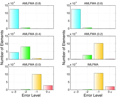
Figure 1. Errors in the matrix-vector multiplications performed by AMLFMA with af in the 0.0–0.8 range and by IMLFMA (omitting the highest level) for a sphere problem discretized with 132,003 unknowns. The reference data is obtained by using an ordinary MLFMA with three digits of accuracy.
Figures 1 and 2 present the number of elements satisfying various base errors for the sphere and patch problems, respectively. Fig. 1 shows that the accuracy of the matrix-vector multiplication deteriorates only slightly when af is 0.8 and 0.6 for the sphere problem, i.e., the base error is −3 or less for most of the elements. Since the ordinary MLFMA has three digits of accuracy, those elements with a base error of less than −2 are considered to be calculated with a high accuracy. Reducing the value of af to 0.4 and 0.2, the accuracy of
AMLFMA decreases and the number of elements satisfying −2 and −1 base errors increases. Finally, when af = 0.0, i.e., when the
truncation number is Tmin for all levels, there are many elements with
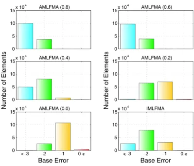
0 base error, which corresponds to at least 10% relative error, which is unacceptably high. Fig. 2 presents similar results for a completely different geometry, i.e., a 20λ × 20λ patch. Using AMLFMA, we are able adjust the accuracy of the matrix-vector multiplications by varying the approximation factor af from 1.0 to 0.0. On the other hand, IMLFMA, which is obtained by omitting only the highest level, provides inaccurate results compared to AMLFMA with af between 0.2 and 0.4 for both problems.
0 5 10 15x 10 4 AMLFMA (0.8) 0 5 10 15x 10 4 AMLFMA (0.6) 0 5 10 15x 10 4 AMLFMA (0.4) Number of Elements 0 5 10 15x 10 4 AMLFMA (0.2) Number of Elements −2 −1 0 5 10 15x 10 4 AMLFMA (0.0) Base Error <−3 −2 −1 0 5 10 15x 10 4 IMLFMA Base Error <−3 0 < 0 <
Figure 2. Errors in the matrix-vector multiplications performed by AMLFMA with af in the 0.0–0.8 range and by IMLFMA (omitting the highest level) for a patch problem discretized with 137,792 unknowns. The reference data is obtained by using an ordinary MLFMA with three digits of accuracy.
Figures 1 and 2 show that we obtain relatively accurate matrix-vector multiplications by AMLFMA when using af in the 0.2–0.4
range. This cannot be predicted by the excess bandwidth formula in (3), which suggests significantly large truncation numbers, as listed in Table 1. This is because the excess bandwidth formula is based on the worst-case scenario for the positions of the basis and testing functions inside the clusters [11]. In fact, the ordinary MLFMA must use the truncation numbers obtained with (3) to guarantee the desired level of accuracy. However, for a typical problem, there are many interactions that can be computed accurately using lower truncation numbers. We employ those interactions in AMLFMA, which can be used to construct powerful preconditioners. Due to the nature of preconditioning, perfect accuracy is not required, instead, the fastest possible solution with the least possible approximation is desired.
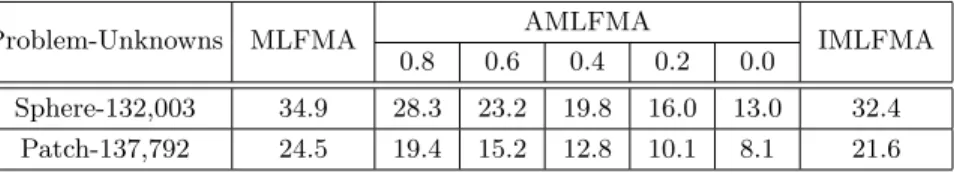
Finally, Table 2 lists the processing time required for a matrix-vector multiplication performed by the ordinary MLFMA, AMLFMA, and IMLFMA, measured on a parallel computer system containing 16 AMD Opteron 870 processors. For both sphere and patch problems,
Table 2. Processing time (seconds) for a single matrix-vector multiplication.
Problem-Unknowns MLFMA AMLFMA IMLFMA
0.8 0.6 0.4 0.2 0.0
Sphere-132,003 34.9 28.3 23.2 19.8 16.0 13.0 32.4 Patch-137,792 24.5 19.4 15.2 12.8 10.1 8.1 21.6
AMLFMA with af = 0.2 provides a significant acceleration by reducing processing time more than 50% compared with the ordinary MLFMA. We also note that the speedup provided by IMLFMA is less than the speedup provided by AMLFMA, even when af = 0.8.
4. PRECONDITIONERS BUILT FROM NEAR-FIELD MATRICES
In MLFMA, there are O(N ) near-field interactions available for the construction of various preconditioners. For example, using the self-interactions of the lowest-level clusters leads to the block-diagonal (BD) preconditioner, which effectively reduces the number of iterations for the combined-field integral equation (CFIE) [1, 15]. On the other hand, the BD preconditioner usually decelerates the iterative solutions of the electric-field integral equation (EFIE) [15]. In addition, for large problems involving complicated objects, acceleration provided by the BD preconditioner may not be sufficient, even when the problems are formulated with CFIE. For the efficient solution of those problems, it is necessary to construct better preconditioners [16] by using all of the available near-field interactions instead of using only the diagonal blocks.
One of the most common preconditioning techniques based on the sparse matrices is the incomplete LU (ILU) method [17]. This is a forward-type preconditioning technique, where the preconditioner matrix M approximates the system matrix, and we solve for
M−1· Z · a = M−1· v (left preconditioning) (7)
or ³
Z · M−1 ´
·¡M · a¢= v (right preconditioning), (8) instead of the original matrix equation Z · a = v. In (7) and (8), the solution of M · x = y for a given y should be cheaper than the solution of the original matrix equation. During the factorization of
the preconditioner matrix, the ILU method sacrifices some of the fill-ins and provides an approximation to the near-field matrix, i.e.,
M = L · U ≈ ZN F. (9)
Recently, we showed that an ILU preconditioner without a threshold provides an inexpensive and good approximation to the solution of the near-field matrix for CFIE, hence it reduces the iteration counts and solution times substantially [18]. For ill-conditioned EFIE matrices, however, ILUT (i.e., threshold-based ILU) with pivoting [19] is required to prevent the potential instability. Other successful adoptions of the ILU preconditioners are presented by Lee et al. [20].
Despite the remarkable success of the ILU preconditioners, they are limited to sequential implementations due to difficulties in paral-lelizing their factorization algorithms and forward-backward solutions. Hence, the sparse-approximate-inverse (SAI) preconditioner that is well-suited for parallel implementations has been more preferable for the solution of large-scale electromagnetics problems [14, 21, 22]. The SAI preconditioner is based on a backward-type scheme, where the in-verse of the system matrix is directly approximated, i.e., M ≈ Z−1. In MLFMA, only the near-field matrix is considered [23], and we minimize
°
°I − M · ZNF°°
F, (10)
where k · kF represents the Frobenius norm. Using the pattern of
the near-field matrix for the nonzero pattern of M provides some advantages by decreasing the number of QR factorizations required during the minimization in (10) [14]. In parallel implementations, we use a row-wise partitioning to distribute the near-field interactions among the processors. Therefore, left-preconditioning must be used to accelerate the iterative solutions with the SAI preconditioner. However, right-preconditioning can also be used for the symmetric matrix equations derived from EFIE [22].
Recently, we showed that the SAI preconditioner is useful in reducing the iteration counts for closed and complicated surfaces formulated with CFIE, as well as open surfaces formulated with EFIE. However, for EFIE, the SAI preconditioner is less successful than the ILU methods, although they are based on the same near-field matrix. As a remedy, we use an inner-outer scheme [6] by employing the SAI preconditioner to accelerate the iterative solution of the near-field system, which is then used as a preconditioner for the full matrix equation [24]. The resulting forward-type preconditioner is called the iterative near-field (INF) preconditioner. Contrary to the ILU preconditioners, which approximate the near-field matrix (M ≈ ZN F), the INF preconditioner employs the near-field matrix
exactly (M = ZN F), but the preconditioner system is solved iteratively and approximately. Since the preconditioner is changed during the iterations, a flexible Krylov-subspace method should be used for the outer solutions [19]. In the next section, we introduce a robust preconditioning technique, which is based on a similar inner-outer scheme, but this time we employ AMLFMA for the inner solutions to construct more effective preconditioners.
5. ITERATIVE PRECONDITIONING BASED ON AMLFMA
Preconditioners that are based on the near-field interactions can be insufficient to accelerate the iterative solutions of large-scale problems, especially those formulated with EFIE. For more efficient solutions, it is possible to use the far-field interactions in addition to the near-field interactions and construct more effective preconditioners. This can be achieved by using flexible solvers and employing approximate and ordinary versions of MLFMA in an inner-outer scheme. Using a reasonable approximation for the inner solutions, the number of outer iterations can be reduced substantially. In addition to more efficient solutions, the inner-outer scheme prevents numerical errors that arise because of the deviations of the computed residual from the true residual by significantly decreasing the number of outer iterations. This is because the “residual gap,” i.e., the difference between the true and computed residuals, increases with the number of iterations [25]. Another benefit of the reduction in iteration counts appears when the iterative solutions are performed with the generalized minimal residual (GMRES) algorithm, which is usually an optimal method for EFIE in terms of the processing time [14, 18]. Even though flexible variants of GMRES, namely, FGMRES [19] or GMRESR [26], require the storage of two vectors per iteration instead of one, nested solutions require significantly less memory than the ordinary GMRES solutions since nested solutions dramatically reduce the iteration counts.
There are many factors that affect the performance of an inner-outer scheme, such as the primary preconditioning operator, the choice of the inner solver and the secondary preconditioner to accelerate the inner solutions, and the inner stopping criteria. Now, we discuss these factors in detail.
5.1. Preconditioning Operator
In an extreme case, one can use the full matrix itself as a preconditioner by employing the ordinary MLFMA to perform the matrix-vector
multiplications for the inner solutions. On the other hand, an inner-outer scheme usually increases the total number of matrix-vector multiplications compared to the ordinary solutions [25]. In addition, an approximate solution instead of an ordinary solution can be sufficient to construct a robust preconditioner. As discussed in Section 3, AMLFMA is an appropriate choice to perform the inner solutions. By using the approximation factor af, the accuracy of AMLFMA can
be adjusted to achieve a maximum overall efficiency.
5.2. Inner Solver and the Secondary Preconditioner
For the inner solutions, GMRES is preferable due to its rapid convergence in a small number of iterations. The inner solutions are also accelerated by using a secondary preconditioner based on the near-field interactions. Among the various choices discussed in Section 4, we prefer the SAI preconditioner, which effectively increases the convergence rate, especially in the early stages of the iterative solutions [14].
5.3. Inner Stopping Criteria
The relative residual error εin and the upper limit for the number
of inner iterations jin
max are also important parameters that affect the
overall efficiency of the inner-outer scheme. Van den Eshof et al. [25] showed that fixing εin is nearly optimal if relaxation is not applied.
However, even 0.1 (10%) residual error can cause a significant number of inner iterations for large-scale problems. Therefore, in addition to εin, the maximum number of iterations jmaxin should be set carefully
to avoid unnecessary iterations during the inner solutions. For large problems, a small value of jin
maxis more likely to keep the inner iteration
counts under control than a large value of εin.
6. NUMERICAL RESULTS
Finally, we demonstrate the performance of the proposed inner-outer scheme using AMLFMA, compared to the solutions accelerated with BD, SAI, and INF preconditioners. Fortran 90 programming language is used for all implementations. Solutions are performed on a distributed-memory parallel computer containing Intel Xeon Harpertown processors with 3.0 GHz clock rate. A total of 32 cores located in 16 nodes (2 cores per node) are used, and the nodes are connected via an Infiniband network. A hierarchical partitioning strategy is used for the parallelization of MLFMA [3].
Iterative solvers, namely, GMRES and FGMRES, are provided by the PETSc library [27]. In all solutions, matrix-vector multiplications are performed by MLFMA with three digits of accuracy. For the inner solutions with AMLFMA, the target residual error and the approximation factor are set to 10−1 and 0.2, respectively. To avoid
unnecessary work, inner solutions are stopped at maximum 10th iteration (jin
max= 10). For the INF preconditioner, however, the target
residual error for the inner solutions is in the range of 10−2 to 10−1,
whereas the maximum number of iterations is set to between 3 and 5, depending on the problem. A small number of inner iterations is usually sufficient for INF since the SAI preconditioner used to accelerate the inner solutions provides a good approximation to ZN F.
Parameters for the preconditioners are determined by testing the implementations on a wide class of problems and choosing the optimal combination to minimize the total processing time for each preconditioner. For example, by setting the approximation factor to 0.2 in AMLFMA, most of the matrix elements are calculated with less than 10% error. Then, using 10−1residual error for the inner iterations
provides the best performance. Choosing a smaller error threshold leads to unnecessary iterations and a larger error threshold wastes the relatively high accuracy of AMLFMA. Setting the maximum number of iterations to more than 10 increases the processing time, even though the accuracy of the inner solutions is not improved significantly.
EFIE is notorious for generating ill-conditioned matrix equations, which are difficult to solve iteratively, especially when the problem size is large [18, 28]. Therefore, the proposed inner-outer scheme employing AMLFMA is particularly useful for open surfaces that must be formulated with EFIE. In addition, we show that the iterative solutions of complicated problems involving closed surfaces that are formulated with CFIE are also improved by the proposed method. 6.1. EFIE Results
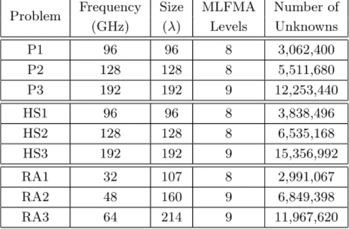
Figure 3 presents three different metallic objects involving open surfaces, namely, a square patch (P), a half sphere (HS), and a reflector antenna (RA). The patch is illuminated by a horizontally-polarized plane wave propagating at 45◦ angle from the normal of the patch. The half sphere and the reflector antenna are illuminated by plane waves propagating along the axes of symmetry of these objects. Discretizations of the objects for various frequencies lead to large matrix equations with millions of unknowns, as listed in Table 3. Dimensions of the objects in terms of the wavelength and the number of active levels (L) in MLFMA are also listed in Table 3.
Patch (P) Half Sphere (HS)
Reflector Antenna (RA)
Figure 3. Metallic objects modeled with open surfaces.
Table 3. Electromagnetics problems involving open metallic objects. Problem Frequency Size MLFMA Number of
(GHz) (λ) Levels Unknowns P1 96 96 8 3,062,400 P2 128 128 8 5,511,680 P3 192 192 9 12,253,440 HS1 96 96 8 3,838,496 HS2 128 128 8 6,535,168 HS3 192 192 9 15,356,992 RA1 32 107 8 2,991,067 RA2 48 160 9 6,849,398 RA3 64 214 9 11,967,620
Table 4 presents the number of iterations and the processing time for the solutions of the problems in Table 3. We observe that using the INF preconditioner accelerates the solutions significantly compared to the SAI preconditioner used alone. Employing the inner-outer scheme with AMLFMA further reduces the processing time, and we are able to solve the largest problem discretized with about 12 million unknowns in less than 7 hours. Although not shown in Table 4, the memory required for the iterative algorithm is also reduced substantially by the proposed method since the memory requirements of both GMRES and FGMRES increase with the number of iterations. As an example, for the solution of P3 with SAI, GMRES requires 2614 MB per processor. Using an inner-outer scheme and AMLFMA, the memory requirement is reduced to 820 MB.
Table 4. Processing time (seconds) and the number of iterationsa
for the solution of electromagnetics problems involving open metallic objects.
Problem SAI
b SAI INF AMLFMA
Setup Outer Time Outer Inner Time Outer Inner Time P1 132 194 6,225 131 391 4,393 35 345 3,278 P2 308 234 27,902 160 478 19,620 43 425 9,860 P3 1,136 276 36,677 174 868 25,650 52 516 17,454 HS1 350 480 23,458 367 1,101 18,374 68 680 11,085 HS2 839 546 66,778 406 1,218 51,285 75 750 23,143 HS3 5,620 357 59,734 276 1,380 48,786 51 510 31,740 RA1 201 200 7,276 138 408 5,138 33 327 4,233 RA2 671 252 31,784 172 509 22,404 42 417 13,746 RA3 2,077 336 43,912 228 1,138 32,710 57 567 24,595 aThe relative residual error is 10−3 for HS3 and RA3, and 10−6 for other
problems.
bSetup of the SAI preconditioner is also required for INF and AMLFMA.
Helicopter (H) Flamme (F)
Figure 4. Metallic objects modeled with closed surfaces. 6.2. CFIE Results
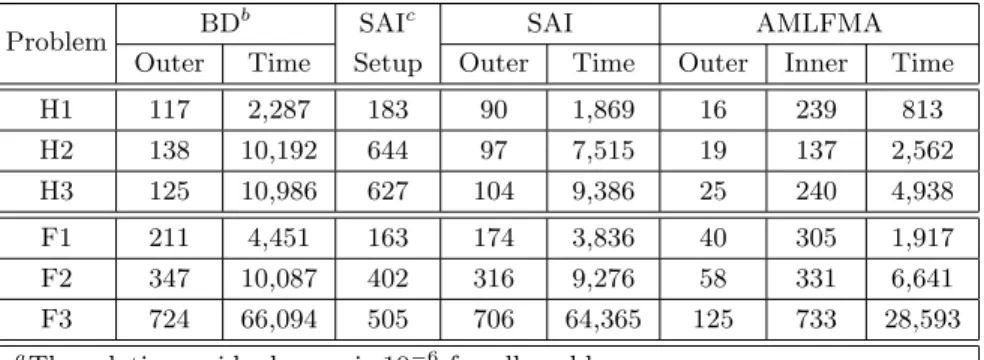
Figure 4 presents two objects modeled with closed conducting surfaces, namely, a helicopter (H) and a stealth airborne target named Flamme (F) [29]. The Flamme is illuminated by a plane wave propagating towards the nose of the target, whereas the helicopter is illuminated from the top. Electromagnetics problems involving those objects in Fig. 4 and listed in Table 5 are formulated with CFIE (α = 0.2). Table 6 presents the number of iterations and the processing time when the solutions are accelerated with the BD and SAI preconditioners, as well as the inner-outer scheme using
Table 5. Electromagnetics problems involving closed metallic objects. Problem Frequency Size MLFMA Number of
(GHz) (λ) Levels Unknowns F1 40 80 8 1,248,480 F2 60 120 8 3,166,272 F3 80 160 9 4,993,920 H1 1.7 96 8 1,302,660 H2 2.4 136 9 2,968,512 H3 3.4 193 9 5,210,640
Table 6. Processing time (seconds) and the number of iterationsa
for the solution of electromagnetics problems involving closed metallic objects.
Problem BD
b SAIc SAI AMLFMA
Outer Time Setup Outer Time Outer Inner Time
H1 117 2,287 183 90 1,869 16 239 813 H2 138 10,192 644 97 7,515 19 137 2,562 H3 125 10,986 627 104 9,386 25 240 4,938 F1 211 4,451 163 174 3,836 40 305 1,917 F2 347 10,087 402 316 9,276 58 331 6,641 F3 724 66,094 505 706 64,365 125 733 28,593 aThe relative residual error is 10−6for all problems.
bThe BD preconditioner has a negligible setup time.
cSetup of the SAI preconditioner is also required for AMLFMA.
AMLFMA. We observe that the proposed method reduces the solution time significantly compared to both the BD and SAI preconditioners. 7. CONCLUSION
MLFMA enables the iterative solution of very large problems in electromagnetics. However, achieving a rapid convergence in a reasonable iteration count is only viable by means of robust preconditioners. In the context of MLFMA, the general trend is to develop sparse preconditioners by using the near-field interactions. However, as the problem size gets larger and the number of unknowns also increases, those preconditioners become sparser and they may not be sufficient to obtain an efficient solution.
In this paper, we propose an inner-outer scheme to improve iterative solutions with MLFMA. For the inner solutions, matrix-vector multiplications are performed efficiently by AMLFMA, which is obtained by systematically reducing the accuracy of the ordinary MLFMA. We show that the resulting solver accelerates the iterative solutions of electromagnetics problems involving open and closed geometries formulated with EFIE and CFIE, respectively.
ACKNOWLEDGMENT
This work was supported by the Scientific and Technical Research Council of Turkey (TUBITAK) under Research Grants 105E172 and 107E136, the Turkish Academy of Sciences in the framework of the Young Scientist Award Program (LG/TUBA-GEBIP/2002-1-12), and by contracts from ASELSAN and SSM. ¨Ozg¨ur Erg¨ul was also supported by a Research Starter Grant provided by the Faculty of Science at the University of Strathclyde.
REFERENCES
1. Song, J., C.-C. Lu, and W. C. Chew, “Multilevel fast multipole algorithm for electromagnetic scattering by large complex objects,” IEEE Trans. Antennas Propagat., Vol. 45, No. 10, 1488– 1493, Oct. 1997.
2. Coifman, R., V. Rokhlin, and S. Wandzura, “The fast multipole method for the wave equation: A pedestrian prescription,” IEEE Antennas Propag. Mag., Vol. 35, No. 3, 7–12, Jun. 1993.
3. Erg¨ul, ¨O. and L. G¨urel, “A hierarchical partitioning strategy for efficient parallelization of the multilevel fast multipole algorithm,” IEEE Trans. Antennas Propagat., Vol. 57, No. 6, 1740–1750, Jun. 2009.
4. Taboada, J. M., M. G. Araujo, J. M. Bertolo, L. Landesa, F. Obelleiro, and J. L. Rodriguez, “MLFMA-FFT parallel algo-rithm for the solution of large-scale problems in electromagnetics,” Progress In Electromagnetics Research, Vol. 105, 15–30, 2010. 5. Bouras, A. and V. Frayss´e, “Inexact matrix-vector products in
Krylov methods for solving linear systems: A relaxation strategy,” SIAM J. Matrix Anal. Appl., Vol. 26, No. 3, 660–678, 2005. 6. Simoncini, V. and D. B. Szyld, “Flexible inner-outer Krylov
subspace methods,” SIAM J. Numer. Anal., Vol. 40, No. 6, 2219– 2239, 2003.
7. Ding, D. Z., R. S. Chen, and Z. H. Fan, “SSOR preconditioned inner-outer flexible GMRES method for MLFMA analysis of scattering of open objects,” Progress In Electromagnetics Research, Vol. 89, 339–357, 2009.
8. Chew, W. C., J.-M. Jin, E. Michielssen, and J. Song, Fast and Efficient Algorithms in Computational Electromagnetics, Artech House, Boston, MA, 2001.
9. Rao, S. M., D. R. Wilton, and A. W. Glisson, “Electromagnetic scattering by surfaces of arbitrary shape,” IEEE Trans. Antennas Propagat., Vol. 30, No. 3, 409–418, May 1982.
10. Koc, S., J. M. Song, and W. C. Chew, “Error analysis for the numerical evaluation of the diagonal forms of the scalar spherical addition theorem,” SIAM J. Numer. Anal., Vol. 36, No. 3, 906– 921, 1999.
11. Hastriter, M. L., S. Ohnuki, and W. C. Chew, “Error control of the translation operator in 3D MLFMA,” Microwave Opt. Technol. Lett., Vol. 37, No. 3, 184–188, Mar. 2003.
12. Erg¨ul, ¨O. and L. G¨urel, “Optimal interpolation of translation operator in multilevel fast multipole algorithm,” IEEE Trans. Antennas Propagat., Vol. 54, No. 12, 3822–3826, Dec. 2006. 13. Brandt, A., “Multilevel computations of integral transforms
and particle interactions with oscillatory kernels,” Comp. Phys. Comm., Vol. 65, 24–38, Apr. 1991.
14. Carpentieri, B., I. S. Duff, L. Giraud, and G. Sylvand, “Combining fast multipole techniques and an approximate inverse preconditioner for large electromagnetism calculations,” SIAM J. Sci. Comput., Vol. 27, No. 3, 774–792, 2005.
15. Erg¨ul, ¨O. and L. G¨urel, “Iterative solutions of hybrid integral equations for coexisting open and closed surfaces,” IEEE Trans. Antennas Propag., Vol. 57, No. 6, 1751–1758, Jun. 2009.
16. Araujo, M. G., J. M. Bertolo, F. Obelleiro, and J. L. Rodriguez, “Geometry based preconditioner for radiation problems involving wire and surface basis functions,” Progress In Electromagnetics Research, Vol. 93, 29–40, 2009.
17. Benzi, M., “Preconditioning techniques for large linear systems: A survey,” J. Comput. Phys., Vol. 182, No. 2, 418–477, Nov. 2002. 18. Malas, T. and L. G¨urel, “Incomplete LU preconditioning with the multilevel fast multipole algorithm for electromagnetic scattering,” SIAM J. Sci. Comput., Vol. 29, No. 4, 1476–1494, Jun. 2007.
Philadelphia, 2003.
20. Lee, J., J. Zhang, and C.-C. Lu, “Incomplete LU preconditioning for large scale dense complex linear systems from electromagnetic wave scattering problems,” J. Comput. Phys., Vol. 185, No. 1, 158–175, Feb. 2003.
21. Lee, J., J. Zhang, and C.-C. Lu, “Sparse inverse preconditioning of multilevel fast multipole algorithm for hybrid integral equations in electromagnetics,” IEEE Trans. Antennas and Propagat., Vol. 52, No. 9, 2277–2287, Sep. 2004.
22. Malas, T. and L. G¨urel, “Accelerating the multilevel fast multipole algorithm with the sparse-approximate-inverse (SAI) preconditioning,” SIAM J. Sci. Comput., Vol. 31, No. 3, 1968– 1984, Mar. 2009.
23. Ding, D. Z., R. S. Chen, and Z. H. Fan, “An efficient SAI preconditioning technique for higher order hierarchical MLFMA implementation,” Progress In Electromagnetics Research, Vol. 88, 255–273, 2008.
24. G¨urel, L. and T. Malas, “Iterative near-field (INF) preconditioner for the multilevel fast multipole algorithm,” SIAM J. Sci. Comput., accepted for publication.
25. Van den Eshof, J., G. L. G. Sleijpen, and M. B. van Gijzen, “Relaxation strategies for nested Krylov methods,” J. Comput. Appl. Math., Vol. 177, No. 2, 347–365, May 2005.
26. Van der Vorst, H. and C. Vuik, “GMRESR: A family of nested GMRES methods,” Numer. Linear Algebra Appl., Vol. 1, No. 4, 369–386, Jul. 1994.
27. Balay, S., W. D. Gropp, L. C. McInnes, and B. F. Smith, PETSc Users Manual, Tech. Report ANL-95/11 — Revision 2.1.5, Argonne National Laboratory, 2004.
28. Carpentieri, B., I. S. Duff, and L. Giraud, “Experiments with sparse preconditioning of dense problems from electromagnetic applications,” Tech. Report TR/PA/00/04, CERFACS, Toulouse, France, 1999.
29. G¨urel, L., H. Ba˜gcı, J.-C. Castelli, A. Cheraly, and F. Tardivel, “Validation through comparison: Measurement and calculation of the bistatic radar cross section of a stealth target,” Radio Science, Vol. 38, No. 3, 12-1–12-10, Jun. 2003.