NOVEL METHODS FOR SAR IMAGING
PROBLEMS
a dissertation submitted to
the department of electrical and electronics
engineering
and the Graduate School of engineering and science
of bilkent university
in partial fulfillment of the requirements
for the degree of
doctor of philosophy
By
Salih U˘
gur
June, 2013
I certify that I have read this thesis and that in my opinion it is fully adequate, in scope and in quality, as a dissertation for the degree of Doctor of Philosophy.
Prof. Dr. Orhan Arıkan (Advisor)
I certify that I have read this thesis and that in my opinion it is fully adequate, in scope and in quality, as a dissertation for the degree of Doctor of Philosophy.
Assoc. Prof. Dr. Sinan Gezici
I certify that I have read this thesis and that in my opinion it is fully adequate, in scope and in quality, as a dissertation for the degree of Doctor of Philosophy.
I certify that I have read this thesis and that in my opinion it is fully adequate, in scope and in quality, as a dissertation for the degree of Doctor of Philosophy.
Prof. Dr. Enis C. etin
I certify that I have read this thesis and that in my opinion it is fully adequate, in scope and in quality, as a dissertation for the degree of Doctor of Philosophy.
Assoc. Prof. Dr. Ali Cafer G¨urb¨uz
Approved for the Graduate School of Engineering and Science:
Prof. Dr. Levent Onural Director of the Graduate School
ABSTRACT
NOVEL METHODS FOR SAR IMAGING PROBLEMS
Salih U˘gur
Ph.D. in Electrical and Electronics Engineering Supervisor: Prof. Dr. Orhan Arıkan
June, 2013
Synthetic Aperture Radar (SAR) provides high resolution images of terrain reflec-tivity. SAR systems are indispensable in many remote sensing applications. High resolution imaging of terrain requires precise position information of the radar platform on its flight path. In target detection and identification applications, imaging of sparse reflectivity scenes is a requirement. In this thesis, novel SAR image reconstruction techniques for sparse target scenes are developed. These techniques differ from earlier approaches in their ability of simultaneous image reconstruction and motion compensation. It is shown that if the residual phase error after INS/GPS corrected platform motion is captured in the signal model, then the optimal autofocused image formation can be formulated as a sparse reconstruction problem. In the first proposed technique, Non-Linear Conjugate Gradient Descent algorithm is used to obtain the optimum reconstruction. To increase robustness in the reconstruction, Total Variation penalty is introduced into the cost function of the optimization. To reduce the rate of A/D conversion and memory requirements, a specific under sampling pattern is introduced. In the second proposed technique, Expectation Maximization Based Matching Pursuit (EMMP) algorithm is utilized to obtain the optimum sparse SAR reconstruction. EMMP algorithm is greedy and computationally less complex resulting in fast SAR image reconstructions. Based on a variety of metrics, performances of the proposed techniques are compared. It is observed that the EMMP algorithm has an additional advantage of reconstructing off-grid targets by perturbing on-grid basis vectors on a finer grid.
Keywords: Synthetic Aperture Radar, Phase Error Correction, Compressed
¨
OZET
SAR G ¨
OR ¨
UNT ¨
ULEME PROBLEMLER˙I ˙IC
¸ ˙IN YEN˙I
METODLAR
Salih U˘gur
Elektrik Elektronik M¨uhendisli˘gi, Doktora Tez Y¨oneticisi: Prof. Dr. Orhan Arıkan
Haziran, 2013
Sentetik Ac.ıklıklı Radar (SAR) y¨uzey yansımasının y¨uksek c.¨oz¨un¨url¨ukl¨u g¨or¨unt¨us¨un¨u sa˘glar. SAR sistemleri pek c.ok uzaktan algılama uygulamasının vazgec.ilmezi olmus.tur. Y¨uzeyin y¨uksek c.¨oz¨un¨url¨ukl¨u g¨or¨unt¨ulenmesi radar platformu uc.us. rotasının hassas pozisyon bilgisini gerektirir. Hedef tespit ve tanımlama uygulamalarında seyrek yansıtıcı y¨uzeylerin g¨or¨unt¨ulenmesi gerekir. Bu tezde, seyrek hedef y¨uzeyleri ic.in yeni SAR g¨or¨unt¨u geric.atımı teknikleri gelis.tirilmis.tir. Bu teknikler daha ¨oncekilerden, g¨or¨unt¨u olus.turulması ve plat-form hareket hatalarının giderilmesi is.lemlerinin es. zamanlı yapılmaları ac.ısından farklılas.maktadır. Platform hareketinin INS/GPS yardımıyla d¨uzeltilmesi son-rası kalan faz bozuklu˘gunun sinyal modeline katılmasıyla, en iyi otomatik odaklanmıs. g¨or¨unt¨u olus.turulması is.lemi bir seyrek geri c.atım problemi olarak ortaya konulmaktadır. ˙Ilk ¨onerilen teknikte, eniyi geri c.atımı elde etmek ic.in Do˘grusal Olmayan Es.lenik Bayır K¨uc.¨ulme algoritması kullanılmaktadır. Geric.atımın g¨urb¨uzl¨u˘g¨un¨un arttırılması amacıyla Toplam De˘gis.im cezası da eniy-ilemenin maliyet fonksiyonuna eklenmis.tir. Analog/sayısal c.eviricilerinin hız ve hafıza gereksinimlerini d¨us.¨urebilmek amacıyla ¨ozel bir alt ¨ornekleme yapısı gelis.tirilmis.tir. Onerilen ikinci teknik, eniyi seyrek SAR g¨¨ or¨unt¨u geric.atımı ic.in Enb¨uy¨ult¨um¨u Tabanlı Uyumlama Takibi algoritmasını kullanmaktadır. Enb¨uy¨ult¨um¨u Tabanlı Uyumlama Takibi algoritması fırsatc.ı bir algoritma olup daha az hesaplama karmas.ıklı˘gı ic.ermektedir ve bu sayede hızlı SAR g¨or¨unt¨u geri c.atımına olanak vermektedir. ¨Onerilen tekniklerin performansları muhtelif perfor-mans parametreleri baz alınarak kars.ılas.tırılmıs.tır. Enb¨uy¨ult¨um¨u Tabanlı Uyum-lama Takibi algoritmasının ek bir avantajı k¨uc.¨uk de˘gis.ikliklerle ızgara ¨uzerinde olmayan hedeflerin geri c.atımına da olanak vermesidir.
Anahtar s¨ozc¨ukler : Sentetik Ac.ıklıklı Radar, Faz Hatası D¨uzeltimi, Sıkıs.tırılmıs.
Acknowledgement
First of all, I would like to thank my advisor, Prof. Dr. Orhan Arıkan whose guidance has made it possible to write this doctoral thesis. His unconditional help and support encouraged me to start, continue, and finish my research twelve years after from leaving university.
I would like to thank members of the thesis monitoring committee, Assoc. Prof. Dr. Sinan Gezici and Assoc. Prof. Dr. Selim Aksoy for their insightful discussions and suggestions. Besides, I would like to thank my Ph. D. thesis defense jury members, Assoc. Prof. Dr. U˘gur G¨ud¨ukbay, Prof. Dr. Enis C. etin, and Assoc. Prof. Dr. Ali Cafer G¨urb¨uz for carefully reviewing and commenting on my thesis.
I would also like to thank my parents to whom I owe everything. I appreciate indulgence of my beloved daughter Dilara and son ¨Omer towards their ever-busy father.
Finaly, I would like to thank my wife Deniz for her support and patience during all my studies.
Contents
1 Introduction 1
1.1 SAR Data Acquisition . . . 4 1.2 Phase Error Due To Platform Motion in SAR . . . 7 1.3 SAR Motion Compensation by Phase Gradient Autofocus Technique 10
2 SAR Image Reconstruction and Autofocus by Compressed
Sens-ing 13
2.1 Compressed Sensing: A Short Review . . . 15 2.2 SAR Raw Data Sampling Technique for Compressed Sensing
Ap-plications . . . 17 2.3 The Proposed Autofocused Sparse SAR Image Reconstruction
Technique in the Compressed Sensing Framework . . . 19 2.4 Results of the Proposed Technique on Synthetic and Real SAR
Data . . . 22 2.4.1 Synthetic Data Reconstructions . . . 23 2.4.2 MSTAR Reconstructions . . . 25
CONTENTS viii
3 Autofocused Sparse SAR Image Reconstruction by EMMP
Al-gorithm 32
3.1 Simultaneous Reconstruction and Autofocus of Sparse SAR Images
Based on EMMP Algorithm . . . 33
3.2 Simulation Results . . . 37
3.2.1 Synthetic Data Results . . . 39
3.2.2 Slicy Data Results . . . 39
3.3 Effect of Sparsity Parameter on Image Reconstruction Quality of the Proposed Technique Based on EMMP Algorithm . . . 43
3.4 Comparison of Sparse SAR Image Reconstruction Performances of the Techniques Based on EMMP and Non-Linear Conjugate Gradient Descent Algorithms . . . 45
4 Off-Grid Sparse SAR Image Reconstruction Based on EMMP Algorithm 50 4.1 Proposed Off-Grid Sparse SAR Image Reconstruction Technique Based on EMMP Algorithm . . . 52
4.2 Simulations . . . 55
5 Conclusions and Future Work 59
Bibliography 62
List of Figures
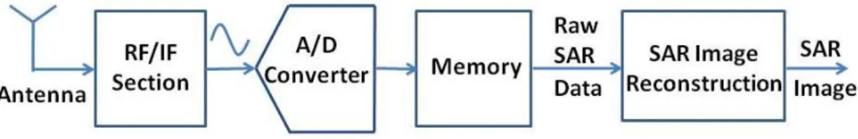
1.1 Typical SAR image formation process. . . 2
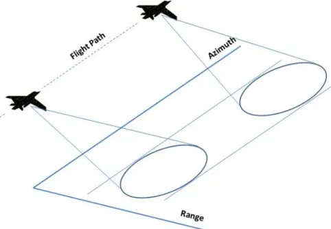
1.2 Strip mode SAR geometry. . . 3
1.3 Spot mode SAR geometry. . . 3
1.4 Spotlight mode SAR imaging geometry. . . 5
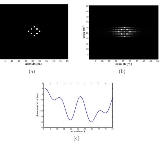
1.5 (a) Synthetically generated SAR image. (b) SAR image with phase error. (c) Added phase error in radians. . . 9
1.6 PGA algorithm: PGA is applied to complex valued image data. It finds and center shifts the most powerful scatterers in each range bin. After applying windowing and transforming the data to range compressed domain, PGA estimates the phase error. These steps are repeated for a fixed number of times or until a certain threshold is reached. . . 11
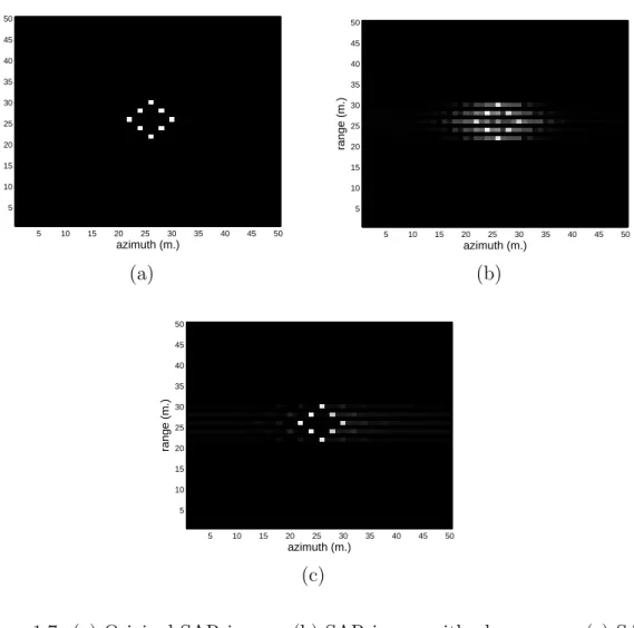
1.7 (a) Original SAR image. (b) SAR image with phase error. (c) SAR image reconstructed by PFA and autofocused by using PGA technique. . . 12
LIST OF FIGURES x
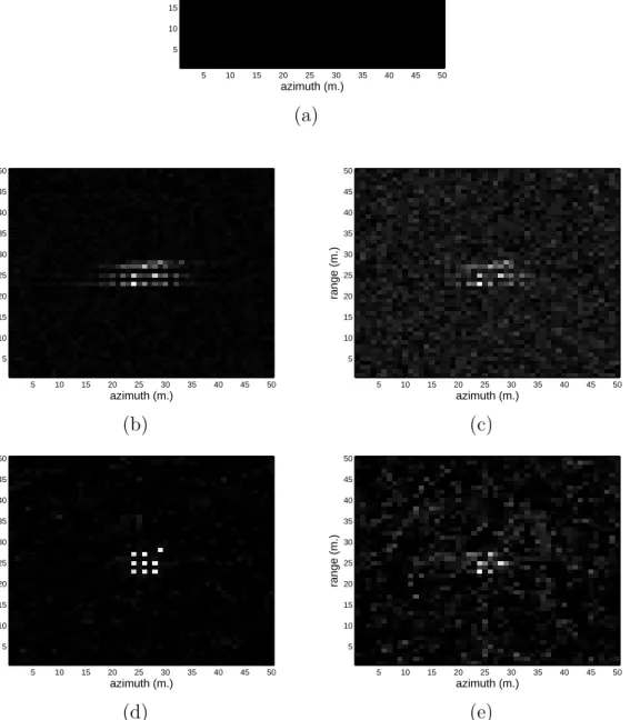
2.2 The synthetic images by PFA and the reconstructions by CS-PE-TV are illustrated. (a) Original reflectivity image. (b) Image with phase error and speckle noise (SNR = 31 dB) reconstructed by PFA. (c) Image with phase error and speckle noise (SNR = 19 dB) reconstructed by PFA. (d) Image with phase error and speckle noise (SNR = 31 dB) reconstructed by CS-PE-TV. (e) Image with phase error and speckle noise (SNR = 19 dB) reconstructed by CS-PE-TV. . . 24 2.3 Three target images of MSTAR database that are used in the trials.
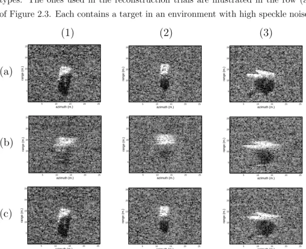
All the images are reconstructed by PFA. Row (a) gives the original images. Row (b) presents the images with inserted phase error. Row (c) shows the reconstructions of images autofocused by PGA. 25 2.4 Three target images of MSTAR database that are used in the trials.
Row (a) gives the results of CS reconstructions. Row (b) presents the results of CS-PE reconstructions. Row (c) gives the images reconstructed by CS-PE-TV. . . 26 2.5 The phase error applied to the image (solid line) and the phase
error estimate (dotted line). Y-axis units represent the fractions of the SAR wavelength. . . 28
3.1 EMMP algorithm with phase error estimation. . . 38 3.2 The synthetic target reconstructions are illustrated. (a) The
orig-inal image reconstructed by PFA. (b) The origorig-inal image with in-serted phase error. (c) The autofocused image by PGA. (d) Image reconstructed by the proposed technique. While the images (a), (b) and (c) use data obtained at the Nyquist rate, for (d) the EMMP uses only 30% of the Nyquist rate data. . . 40
LIST OF FIGURES xi
3.3 Two Slicy target reconstructions are shown in two columns. First row: PFA reconstructions with no phase errors; Second row: PFA reconstructions with synthetically induced phase errors; Third row: PFA-PGA reconstructions; Fourth row: proposed EMMP recon-structions. While PFA and PFA-PGA use data obtained at the Nyquist rate, in Slicy target reconstructions the EMMP uses only 22.5% of the Nyquist rate data. . . . 41 3.4 The synthetic (solid line) and the estimated phase error (dashed
line) in radians. . . 42 3.5 The effect of the sparsity parameter, K on image reconstructions
by the proposed EMMP technique is illustrated. A military target image from MSTAR database is used for the trials. Only 40% of the Nyquist rate data is used for the reconstructions by the proposed technique. (a) Original image, (b) K = 30, (c) K = 40, (d) K = 50, (e) K = 70, and (f) K = 80. . . . 44 3.6 Three target images of MSTAR database that are used in the trials.
Row (a) gives the original images reconstructed by PFA. Row (b) presents the images with inserted phase error and reconstructed by PFA. Row (c) gives the images reconstructed PFA and auto-focused by PGA. Row (d) gives the images reconstructed by CS-PE-TV technique. Row (e) shows the images reconstructed and autofocused by the proposed technique based on EMMP algorithm. 46
4.1 Off-grid and on-grid points on a discrete grid. . . 51 4.2 The proposed SAR-EMMP algorithm . . . 53
LIST OF FIGURES xii
4.3 Grid points for the reconstruction of the basis vectors. For the first run of the EMMP algorithm the points with full circles are used to reconstruct the basis vectors. The first run gives the on-grid point estimates. Around that point, resolution is increased by constructing a finer grid. Hence, for the second run of the EMMP algorithm the points with empty circles are used to reconstruct the basis vectors. . . 54 4.4 The image reconstructed by PFA. The pixel resolution is 1 m. in
both azimuth and range directions. . . 56 4.5 The image reconstructed by the technique using Non-Linear
Con-jugate Gradient Descent algorithm which is detailed in the Chap-ter 2. The pixel resolution is 1 m. in both azimuth and range directions. . . 56 4.6 The image reconstructed by EMMP algorithm with sparsity
pa-rameter K = 5. The pixel resolution is 1 m. in both azimuth and range directions. . . 57 4.7 The image reconstructed by EMMP algorithm with sparsity
pa-rameter K = 10. The pixel resolution is 1 m. in both azimuth and range directions. . . 58
List of Tables
2.1 A/D rate and the memory requirement for different values of pa-rameters K and L. . . . 19 2.2 Performance metrics for the imagery reconstructed by different
methods. . . 29
3.1 Metrics for the Slicy target imagery reconstructed by PFA-PGA and the proposed EMMP techniques. The PFA-PGA technique, which is reconstructed by PFA and autofocused by PGA uses whole raw SAR data. The proposed EMMP technique uses only 22.5% of the Nyquist rate data. . . 43 3.2 Effect of sparsity parameter on image reconstruction quality
met-rics. A military target image from MSTAR database is used for the trials. Only 40% of the raw data is used for the reconstructions by the proposed technique. . . 45 3.3 Comparison of performance metrics for the imagery reconstructed
by techniques PFA-PGA, CS-PE-TV, and EMMP. . . 48
4.1 The actual and resulting coordinates of the off-grid reflectivity cen-ters. . . 55
Chapter 1
Introduction
Synthetic Aperture Radar (SAR) systems provide high resolution images of ter-rain reflectivity. Typically, an airborne or spaceborne platform carries a monos-tatic radar system on a straight flight path, while the radar transmits and receives echoes from the area of interest. The received and digitized radar returns are co-herently processed to obtain significantly higher resolutions in azimuth direction that could have been obtained by a large aperture antenna.
SAR systems are widely used in ground surveillance, terrain mapping and environmental monitoring applications due to their ability to provide high reso-lution images. They have wide range of users from commercial, scientific, and military fields. Commercial users focus on the manage and monitor the Earth’s resources while scientific users has a much wider range from monitoring global cli-mate change to discovering leakage detection on the sea. In military applications, SAR is primarily used in intelligence, surveillance and reconnaissance (ISR) mis-sions. Increased demand on high precision ISR outputs requires sub-meter or even higher resolutions from SAR images. High resolution SAR systems are becom-ing competitive alternatives and supplements of Electro-Optic/Infrared (EO/IR) cameras for ISR applications. Also, capability of operating in all weather condi-tions makes them very appealing for surveillance applicacondi-tions where performance of EO/IR cameras heavily depend on the atmospheric conditions and time of the day.
In a typical digital SAR image reconstruction processing chain, the received analog signal is first down-converted and sampled by using an A/D converter operating above the Nyquist rate of sampling (Figure 1.1). The sampling rate of
Figure 1.1: Typical SAR image formation process.
the A/D converter depends on the bandwidth of the SAR system which deter-mines the range resolution. The A/D converted signal is written in a memory for further processing. The size of the required memory is derived from the data rate of the A/D converter and the processing power of the SAR image formation pro-cessor. The stored data is either processed in real-time by an on-board processor or transferred by a data link to a ground station where the image formation takes place.
SAR range resolution depends on the bandwidth of the transmitted signal similar to classical radars. High bandwidth results finer resolution. Azimuth resolution in SAR depends on the synthetic aperture length. Longer aperture provides finer azimuth resolution.
SAR has two main modes, namely stripmap and spotlight. In stripmap mode SAR (Figure 1.2), the radar antenna angle with respect to platform route is held constant. It gives the strip image of larger scenes in coarser resolutions. In spotlight mode SAR (Figure 1.3), the radar antenna is directed to a constant position in the imaged scene throughout the data collection phase. In this mode finer resolutions are obtained for relatively small scenes. In military ISR appli-cations, typical SAR mission flow is as follows: First a stripmap mode image of the scanned area is examined usually with the help of a computer to detect possible targets. For detected ones, a spotlight mode mission is performed to obtain high resolution images of the targets. The SAR image reconstruction re-quires to collect all the data corresponding to the synthetic aperture. In other
Figure 1.2: Strip mode SAR geometry.
words, reconstruction process waits for the SAR to collect all the data for the corresponding image. Therefore there is a lag between the data collection and re-construction times of the SAR image. Due to this lag, SAR image rere-construction is called as a near-real time process.
Apart form the data collection geometry, SAR modes mainly differ by their respective reconstruction algorithms. A variety of different reconstruction algo-rithms have been proposed for both modes of operation. For stripmap mode, range-Doppler [1, 2, 3], chirp scaling [4], and w− K [5] algorithms are com-monly used techniques. Main feature of range-Doppler algorithm is to perform all operations in one dimension at a time. Chirp scaling algorithm eliminates the interpolator used for range cell migration correction in range-Doppler algorithm.
w− K algorithm corrects range and azimuth frequency dependence of azimuth
range coupling in two dimensional frequency domain. Polar Format Algorithm (PFA) [6] and Filtered Back Projection (FBP) [7, 8] are the algorithms that are widely used in spotlight mode image reconstruction. PFA utilizes the fact that de-ramped SAR phase history signal is the Fourier transformation of the reflectiv-ity of the scene to be imaged. FBP, originated from computer aided tomography, reconstructs SAR image by back propagating received signals collected through the synthetic aperture to imaged scene.
1.1
SAR Data Acquisition
In this part, we will first focus on the characteristics of the SAR data acquisition in spotlight mode operation. Although they can be applied to other modes of operation, our methods, especially the ones using Compresses Sensing (CS) tech-niques assume the SAR is in spotlight mode for the sake of brevity originating from the basic Fourier transform relation between the received signal and the ground reflectance.
In spotlight mode SAR, at regular intervals along the flight path, the radar transmits the real part of a linear frequency modulated (FM) chirp waveform
s(t), which is defined as: s(t) = ej(ω0t+at2), |t| ≤ T 2 0, otherwise (1.1)
where ω0 is the RF carrier frequency in radians, 2a is the FM rate and T is the
pulse duration. At each look angle, θ, which corresponds to a different azimuth
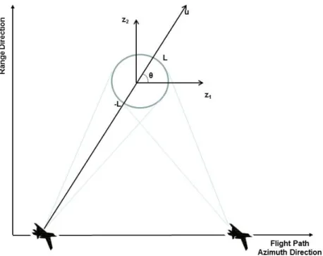
Figure 1.4: Spotlight mode SAR imaging geometry.
position along the synthetic aperture (see Figure 1.4), the relation between the received and demodulated signal yθ(t), and the scene reflectivity x(z1, z2) can be
expressed as [6], yθ(t) = ∫∫ √ z2 1+z22≤L
x(z1, z2) exp{−jΩ(t)(z1cos(θ) + z2sin(θ))}dz1dz2 (1.2)
where L is the spatial extent of the ground patch and
is the radial spatial frequency. Rθ in Ω(t) formulation corresponds to distance
between the platform and the imaged target scene center at a look angle θ. The demodulated signal yθ(t) can also be written as the band-pass filtered Fourier
transform of the projection of the ground reflectivity x(z1, z2) at the angle θ, by
using the projection slice theorem [7]:
yθ(t) =
∫ L
−Lqθ(u) exp{−jΩ(t)u}du, (1.4)
where u is the axis from the platform to the center of the imaged area at the angle θ, and qθ(u) is the projection of the scene reflectivity x(z1, z2) at the angle
θ, given by;
qθ(u) =
∫∫
δ(u− z1cos(θ)− z2sin(θ))x(z1, z2)dz1dz2, (1.5)
and is called the range profile [9]. Matrix based formulation of the spotlight mode SAR image reconstruction problem can be written by discretizing the integral in Eq. 1.2 using its uniform Riemann sum approximation [10]:
yθ = Gθ x, (1.6)
where, x and yθ are vectorized forms of the 2-D ground reflectivity distribution
and the demodulated received signal, respectively. The vectorized form of x is obtained by stacking the columns of the 2-D ground reflectivity distribution matrix and the vectorized form of yθ corresponds to the fast-time samples taken
at the look angle θ. Finally, Gθ is the complex valued discrete SAR projection
operator at the angle θ relating the received signal to the unknown reflectivities. The received signal at each azimuth position is sampled by an A/D converter. All the signals received along the synthetic aperture can be written in a vector form by stacking their respective signal samples. This is achieved by appending the range bins taken from an azimuth location to the bins taken from the next azimuth location. The discretized reflectivity matrix can also be written in a vector form by stacking its respective columns. The relation between the received signal vector and the reflectivity vector then can be written as [9],
where y is the received signal (the measurement vector), G is the complex valued discrete SAR projection operator matrix (composed of all Gθ throughout the
synthetic aperture), x is the reflectivity vector and w is the additive complex white Gaussian measurement noise vector. Assuming N azimuth and N range points results N × N rectangular grid for SAR image. This image has total number of m = N × N pixels. Then, y, x, and w are m × 1 vectors. G is a matrix with size m× m.
1.2
Phase Error Due To Platform Motion in
SAR
SAR systems need accurate distance and angle information between the SAR platform and the reference point in the terrain of interest in order to establish the synthetic aperture precisely. However, especially in airborne SAR applica-tions, due to the limited accuracy of the navigational sensors, there is always some residual error left in the estimation of the actual flight path. These un-compensated platform motion errors cause uncertainties in distance and angle measurements which result in phase errors in the received SAR signal. Let δR represents this measurement error which results mixing error and causes phase errors in the received signal. Hence the demodulation output of Eq. 1.4 becomes [11]:
yθp(t) = ejδR Ω(t)
∫ L
−Lqθ(u) exp{−jΩ(t)u}du = e jϕ(t) y
θ(t), (1.8)
where yθp(t) is the received signal with phase error due to an error of δR in the
platform position from the scene center. Since Ω(t) = (2/c)(ω0+ 2a(t−(2Rθ/c))),
the phase error term ϕ(t), has a constant part and a time varying part. Following Eq. 1.8, the exponential multiplication of the phase error can be inserted to the signal model and the measurement relation of Eq. 1.7 becomes:
Here, Φ is a diagonal matrix representing phase errors for every measurement taken from the imaged scene and is given below,
Φ = ejϕ1 ejϕ2 . .. ejϕm . (1.10)
Here m is the total number of measurements and ϕi’s are the phase errors in
radians incurred at the ith measurement bin. The error in the range compressed data due to phase error is generally ignored, because the resultant range error is typically a small fraction of a range resolution bin [11]. Therefore, phase errors do not depend on the range axis and they are assumed to be the same for all the data corresponding to an azimuth point,
yp1 yp2 .. . ypN = ejϕ1 ejϕ2 . .. ejϕN G1 G2 .. . GN x + w, (1.11)
where ypi is the partition of the measurement vector yp which contains all the
range points corresponding to the azimuth point i, ϕi is the phase error at the
azimuth point i, Gi is the partition of the matrix G corresponding to the range
bins of the azimuth point i and N is the total number of azimuth points. From now on, Gi is used instead of Gθ for representing matrix partition of G in order
not to confuse with angle.
Phase errors are the main cause of degradations in high resolution SAR im-ages limiting achievable performance especially in the azimuth direction. These errors, depending on their nature, can cause geometric distortions, loss of res-olution/contrast, decrease in SNR and even generate spurious targets [6]. An example of a SAR image distorted by phase error is given in Figure 1.5.b. The synthetically generated original image is presented in Figure 1.5.a. Both of these images are reconstructed by PFA. Figure 1.5.c gives the phase error in radians added to the original image.
azimuth (m.) range (m.) 5 10 15 20 25 30 35 40 45 50 5 10 15 20 25 30 35 40 45 50 (a) azimuth (m.) range (m.) 5 10 15 20 25 30 35 40 45 50 5 10 15 20 25 30 35 40 45 50 (b) 0 5 10 15 20 25 30 35 40 45 50 −2 −1.5 −1 −0.5 0 0.5 1 1.5 2 azimuth (m.)
phase error in radians
(c)
Figure 1.5: (a) Synthetically generated SAR image. (b) SAR image with phase error. (c) Added phase error in radians.
Modern SAR systems have high range and azimuth resolutions which ne-cessitate large bandwidths even in excess of 500M Hz. These systems typically requires higher operational frequencies because of the desired bandwidths in the RF and antenna subsystems. Higher operational frequencies increase the required accuracy levels of motion compensation techniques. If not compensated, these motion errors cause greater amount of phase errors at higher frequencies. As a result, higher operational frequencies create significant challenges for autofocus techniques. Furthermore, classical image reconstruction techniques for higher frequency SAR systems require full band, fast A/D converters to digitize the re-ceived signal resulting in larger onboard storage systems. In addition, if the raw data is to be transmitted to another platform for processing, transmission of full band data requires more time or bandwidth.
1.3
SAR Motion Compensation by Phase
Gra-dient Autofocus Technique
SAR platforms are generally equipped with an Inertial Measurement Unit (IMU) to estimate their actual track which can have considerable difference than the planned one. Even when the IMU is used, there is an error left in the estimation of the actual track which causes a phase error in the SAR signal. Autofocus algorithms are image restoration techniques which can be applied to overcome the degradations related to phase errors. There are several autofocus techniques [6, 12, 13, 14, 15, 16, 17, 18, 19, 20] to estimate and correct phase errors by using dedicated algorithms on raw SAR data. These algorithms can be applied to a wide range of SAR images successfully. Once a reliable estimate for the phase error is available, the raw SAR data is corrected to obtain highly improved reconstruc-tions. The autofocus problem is still an active research area in SAR community. The main difficulty in autofocus problem is the nonlinear coupling between the unknown target scene reflectances and the phase error. Recently proposed mod-ern autofocus techniques apply algorithms based on a bilinear parametric model via semidefinite relaxation [21, 22] and claim improved performances over existing
methods.
Phase Gradient Autofocus (PGA) algorithm [18] is a widely used technique to compensate phase error in SAR images. It is a non-parametric estimator and its basic algorithmic steps are given in Figure 1.6[11]. PGA first center shifts
Figure 1.6: PGA algorithm: PGA is applied to complex valued image data. It finds and center shifts the most powerful scatterers in each range bin. After applying windowing and transforming the data to range compressed domain, PGA estimates the phase error. These steps are repeated for a fixed number of times or until a certain threshold is reached.
the brightest pixels on the complex image in each range bin. Then, it applies windowing to suppress the effects of other targets residing in the same range bin. PGA estimates the phase error in the range compressed domain. Then, it applies phase correction using its estimate. These steps are iterated until there is negligible difference between iterations at which point the phase error estimate
is obtained. Usually, around three iterations of the PGA is sufficient to estimate phase errors. The PGA algorithm is applied to the phase error distorted image
azimuth (m.) range (m.) 5 10 15 20 25 30 35 40 45 50 5 10 15 20 25 30 35 40 45 50 (a) azimuth (m.) range (m.) 5 10 15 20 25 30 35 40 45 50 5 10 15 20 25 30 35 40 45 50 (b) azimuth (m.) range (m.) 5 10 15 20 25 30 35 40 45 50 5 10 15 20 25 30 35 40 45 50 (c)
Figure 1.7: (a) Original SAR image. (b) SAR image with phase error. (c) SAR image reconstructed by PFA and autofocused by using PGA technique.
Chapter 2
SAR Image Reconstruction and
Autofocus by Compressed
Sensing
Recent developments in Compressed Sensing (CS) techniques have an impact on the SAR image reconstruction as well. Unlike classical SAR image processing techniques, CS methods can operate on downsampled data to reconstruct SAR images where targets of interest are sparse in a certain transform domain. CS SAR image reconstruction techniques proposed in the literature model the image forming process as a sparse inverse reconstruction problem. In [23, 24], the in-verse problem is formulated as a convex l1 norm minimization and its solution is
obtained by linear programming or approximated by greedy pursuit algorithms. The l1 norm minimization term in the cost function of the convex minimization
problem enforces sparsity. A similar approach is also used in [25] for sparse recon-struction of SAR images which uses the basis pursuit algorithm for the solution of the problem and demonstrates the super resolution property. Several computa-tional tools are available in the literature [26, 27] which can be applied to l1 norm
minimization problems. In [10], the cost function with l1 term is solved by finding
roots on the Pareto curve [26]. But they also modify the reconstruction problem by adding a total variation penalty into the cost function to reduce the speckle
noise effects, which requires development of a dedicated solver. In Fourier imaging applications, the effect of p-norm regularization under amplitude and phase errors is studied in [28], where it is stated that for p < 2 gradient descent optimizations reduce amplitude and phase irregularities. In [29] phase errors are accounted as SAR observation model errors and an iterative sparsity-driven method for simul-taneous SAR imaging and autofocus is proposed. A coordinate descent technique is used to minimize the cost function. This method uses the fully sampled raw data to reconstruct the SAR image. Similarly, joint formulation of SAR recon-struction and autofocus has been proposed in [30], where only 50% of the Nyquist rate samples are used for the processing. There are also several other sparse SAR image reconstruction algorithms that are recently reviewed and compared in [31]. In this chapter, a new CS based sparse SAR image reconstruction technique is proposed. The proposed technique also performs autofocus enabling simulta-neous image reconstruction and correction of phase errors. The proposed tech-nique models the phase error as part of the data acquisition and then employs a CS based approach for image reconstruction and optimal phase error correc-tion. The non-linear conjugate gradient descent algorithm is used to minimize the cost function. In addition to phase error correction, the proposed technique also incorporates total variation (TV) penalty into the cost function, hence it is called as the CS-PE-TV technique. Typical CS applications rely on l1 norm
minimization approaches. However, adding TV penalty into the cost function of the SAR image reconstruction improves the quality of the reconstruction by sup-pressing intensity variations caused by speckle noise, without a smoothing effect on the boundaries [10]. As a novel way of integrating both TV penalty and phase error into the cost function of the sparse SAR image reconstruction problem, the proposed technique improves the overall reconstruction quality.
To facilitate practical implementation, a new under-sampling methodology is presented in this study. It reduces the A/D conversion rate to obtain the required samples for CS SAR image reconstruction, allowing us to overcome the hardware limitations of wide band SAR applications.
2.1
Compressed Sensing: A Short Review
Compressed sensing (CS) is a relatively new signal processing technique [32, 33]. It can provide reliable reconstruction of a signal from a set of linear under-determined measurements. In order to apply CS, the signal should have a sparse representation in a known basis. Since sparsity is encountered in many natural signals, CS has found diverse applications. Consider the following linear mea-surement model:
y = G x, (2.1)
where G is the measurement matrix, y is the measured signal and x is the un-known signal which can be represented sparsely in a un-known basis:
x = Ψ α, (2.2)
where columns of Ψ are basis vectors and α is the vector of sparse representation coefficients. Then Eq. 2.1 can be written as,
y = A α, (2.3)
where A = G Ψ. The sparse solution for the linear model of Eq. 2.1 is found by solving the following l0 norm minimization problem,
min ∥α∥0 such that y = A α, (2.4)
where ∥α∥0 describes the l0 norm which is the number of non-zero entries in α.
The solution to the problem in Eq. 2.4 is combinatorial in nature with prohibitive computational load in practical applications. Convex relaxation of the l0 problem
to the following l1 problem,
min ∥α∥1 such that y = A α, (2.5)
enables use of efficient solution techniques and programming tools for its so-lution [34, 35, 36, 37, 38, 39, 40, 41]. Commonly used sparse reconstruction algorithms are claimed as second order cone programming (SOCP), gradient de-scent approaches, greedy search algorithms, weighted least squares and Bregman iterations.
Uniqueness of the sparse solution of Eq. 2.4 is guaranteed when spark(A)/2≥
∥α∥0 is satisfied [42], where spark of a matrix A is defined as the size of the
small-est linearly dependent column subset. The spark(A) not only controls uniqueness in Eq. 2.4 but also controls it in Eq. 2.5. No sparsity bound implies the equiva-lence of Eqs. 2.4 and 2.5 unless spark(A)/2≥ ∥α∥0. A stronger condition than
the spark of a matrix is the Restricted Isometry Property (RIP), which is defined as,
(1− δs)∥α∥2 ≤ ∥Aα∥2 ≤ (1 + δs)∥α∥2 (2.6)
such that δs> 0, ∥α∥0 < s,
where isometry constant δs satisfies, 0 ≤ δs < 1 [43]. RIP provides an upper
bound for the sparsity of a signal so that its energy is preserved by a given amount through the transformation by the operator. It is proven that Eqs. 2.4 and 2.5 provide the same solution if α is sparse and A holds RIP [43, 44]. Un-fortunately, even for moderate dimensional operators, finding RIP of a given operator is computationally impractical. However, a few classes of matrices are shown to posses RIP almost certainly [33, 43, 44] which include random matri-ces with independent identically distributed entries, Fourier ensemble matrimatri-ces, and general orthogonal measurement ensembles. Note that the general orthogo-nal measurement ensembles can be generated by randomly selecting n rows from
m× m orthonormal matrix and re-normalizing the columns [43].
Application of CS techniques has increased dramatically since its mathemat-ical foundations were laid in 2006 [32, 33]. Medmathemat-ical and electro-optic imaging applications benefit significantly from CS techniques due to the well known bases that are used for sparse representation of the imaged scenes [45]. Applications of CS to radar and SAR are also investigated [23, 24, 25, 10, 31, 46, 47, 48, 49]. The main difficulty in applying CS to SAR imaging is finding an appropriate basis for the sparse representation of SAR images. Due to their speckle noise content, SAR images of terrain cannot be sparsely represented in known domains. Speckle noise is caused by the coherent contributions of multiple distributed reflecting objects in a resolution cell [50]; it creates difficulties in finding sparse basis for SAR im-ages. However, for radar scenes with highly reflective man-made objects, either wavelet or standard basis vectors can be chosen for the sparse representation of
the scene reflectivity distribution [51]. Hence, CS techniques can be applied to SAR image reconstructions of target scenes containing highly reflective objects.
2.2
SAR Raw Data Sampling Technique for
Compressed Sensing Applications
CS techniques recover an S-sparse signal of length N with high probability if the measurement matrix satisfies RIP and the number of measurements are greater than O(S log(N/S)) [52]. Reconstructing a sparse signal with fewer measure-ments than its corresponding Nyquist rate helps reduce the sampling rate and the amount of raw data to be processed. Reduced sampling rates allow usage of slower A/D converters in SAR systems. Furthermore the reduced amount of raw data reduces the memory requirements of the system and the necessary data link bandwidth capacity if the raw data is transferred to a ground segment for image reconstruction.
Using lower rate A/D conversion in wide bandwidth SAR has the same effect as downsampling the original data. However, regular downsampling does not generate measurement matrices with RIP [53]. RIP can be achieved by randomly discarding some of the raw data [25] or any irregular transmission along the flight path [49]. But randomly discarding some of the regularly spaced samples cannot be easily implemented in practice by using lower rate A/D converters. Instead, jittered under-sampling which controls the maximum gap in the data is proposed [54]. First the A/D converter is programmed to sample data on a coarse but uniformly spaced grid. Then at the actual time of sampling, a sampling jitter is used to provide samples that lies almost randomly on a finer grid. Although jittered under-sampling requires accurate jitter control, it provides satisfactory results providing samples similar to desired random under-sampling. Also, a new A/D converter is proposed which performs sub-Nyquist sampling [55]. It presents a new hardware design for A/D converters to be used in CS applications which contain basically an RF front end and classical A/D converters.
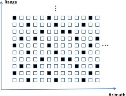
Figure 2.1: Example of the proposed under-sampling pattern for K = 4 .
We propose a simple downsampling scheme that can be implemented using slower rate A/D converters, without any jitter control and hardware change. In this approach, the data is first downsampled by K in the range direction. The time of the initial sample at each azimuth location is pseudo-randomly chosen. This adds randomness to the data in the azimuth direction. Figure 2.1 presents an example of the under-sampling pattern for K = 4. The randomness in the range direction is obtained by randomly discarding a small ratio, L, of the downsampled data. This way, the prerequisites of CS are met despite the loss of a small portion of the data. As a result, this method of under-sampling reduces the rate of the A/D converter by a factor of K and reduces the memory requirement by a factor of (1− L)/K. Table 2.1 lists the reduced A/D rate and the memory requirement for different values of parameters K and L. Note that the first row in the table is given as a reference and indicates the case of original data without any downsampling.
Table 2.1: A/D rate and the memory requirement for different values of param-eters K and L.
K L New A/D rate Memory requirement
1 0 1 100%
2 0.2 1/2 40%
3 0.1 1/3 30%
4 0.1 1/4 22.5%
2.3
The Proposed Autofocused Sparse SAR
Im-age Reconstruction Technique in the
Com-pressed Sensing Framework
The under-sampling scheme described in Section 2.2 results in the following mea-surement relation where the number of meamea-surements is a fraction of the number of unknowns:
yu = Φ Gu x + w, (2.7)
where yu and Gu represent the under-sampled measurement vector and the
pro-jection matrix respectively. Therefore, arbitrary scenes of reflectivity cannot be recovered from the available measurement data. However, if few objects with high reflectivity dominate the scene, sparse reconstruction techniques can provide re-construction of these objects from the available data. Here, Φ also corresponds to the under-sampled phase error matrix but it is not indicated as subscripted by
u for the sake of brevity.
Assume the transformation matrix Ψ transforms the reflectivity vector x to a sparse domain,
In the presence of phase errors, sparse SAR image reconstruction can be formu-lated as a constrained l1 norm minimization problem:
min
Φ,α ∥α∥1 such that ∥yu− ΦAα∥2 ≤ σ, (2.9)
which is known as the Basis Pursuit Denoising (BPDN) formulation. While reconstructing sparse SAR images containing man-made targets, the number of pixels a target covers can be estimated by dividing the size of target area to the area of a pixel in the reconstructed SAR image. With this estimation and the transformation in which the image is sparse, one can set an upper limit τ to the
l1-norm of the target image. Then the SAR image reconstruction problem can
be transformed into the following Lasso formulation [26, 56], min
Φ,α ∥yu− ΦAα∥2 such that ∥α∥1 ≤ τ. (2.10)
By integrating the phase error into the formulation, the required optimization should be carried out in terms of two sets of variables, α and Φ. To obtain an optimal solution, Eq. 2.10 can be solved by first finding optimal Φ for a given α, then transforming the problem to a minimization over α alone [57]. To minimize the cost in Eq.2.10 for a given α, the phase error matrix Φ that minimizes ∥yu− ΦAα∥2 should be obtained. As detailed in Section 1.2 phase
errors are assumed to be the same for all the data corresponding to an azimuth location, resulting in:
min ∥yu−ΦAα∥22 =
N
∑
i=1
min ∥yui− ejϕiAiα∥22, (2.11)
where yuiis the partition of the measurement vector corresponding to the azimuth
point i, Ai is the partition of the matrix A corresponding to the range bins of the
azimuth point i, and N is the total number of azimuth points. Minimization of the term on the left side of the equation requires minimization of the individual terms in the summation, which can be expanded as:
∥yui− ejϕiAiα∥22 = yuiHyui− ejϕiyuiHAiα− e−jϕiαHAiHyui+ αHAiHAiα.
For each term, the minimizing ϕi can be found as:
∂
∂ϕi
∥yui− ejϕiAiα∥22 = j e−jϕiα
HA
iHyui− j ejϕiyuiHAiα = 0. (2.13)
The unique solution for ϕi can be obtained as:
ˆ
ϕi = ̸ (αH AiH yui). (2.14)
With this result, Eq.2.10 can be reduced to an optimization over α only: min
α ∥yu− ΦAα∥2 such that ∥α∥1 ≤ τ, ϕi = ̸ (α
H A
iH yui). (2.15)
The same approach can also be applied for the BPDN formulation given in Eq. 2.9. Note that, since the min-min problem is not convex, the optimization in Eq. 2.15 has a non-convex feasible set. Therefore, local search techniques typically con-verge to a local minima of the problem. If the cost surface is such that the cost of the local minima is significantly higher than the global minima, a global opti-mization technique should be used. As illustrated in the next section, obtained results indicate that the cost of the local minima obtained by the proposed ap-proach and the cost of the global minimum are acceptably close; therefore a slower converging global optimization technique such as Particle Swarm Optimization is not utilized for this problem.
At this stage of the formulation, to further improve the image reconstruction quality, TV penalty is integrated into the cost function [53, 58, 59, 60, 61]. In-tegrated TV penalty smooths the target and its environment and hence reduces the noise content of the image, which also increases the effectiveness of the phase error correction. By adding TV penalty, the cost function becomes:
min
x ∥yu− Φ Gux∥2+ β T V (x) (2.16)
such that ∥ΨHx∥1 ≤ τ, ϕi = ̸ (xH GuiH yui).
Note that the relations α = ΨHx and Aα = Gux are used. Here, TV stands for
total variation and defined as,
T V (x) =∑
i,j
√
where subscripts i, j denote pixel locations in a two dimensional image. ∇i and
∇j denote discrete gradients of the image in two directions and are given by,
(∇ix)i,j = x(i, j) − x(i − 1, j), (2.18)
(∇jx)i,j = x(i, j) − x(i, j − 1). (2.19)
The constrained optimization problem of Eq. 2.3 can be written as an uncon-strained problem in the Lagrangian form:
arg min
x g(x) = ∥Ψ
Hx∥
1+ β T V (x) + γ ∥yu− Φ Gux∥22 (2.20)
such that : ϕi = ̸ (xH GuiH yui), 1≤ i ≤ N.
By using the non-linear conjugate gradient descent algorithm with backtracking line search [53, 62], a numerical solution to Eq. 2.20 can be obtained. There are more efficient algorithms published in the literature to solve l1 minimization
problems. The ones using Bregman methods are especially promising [63, 64, 65]. However, in all these techniques, the transformation in the data fidelity part of the cost function is a known matrix. But in our case, there is non-linear coupling between unknown reflectances and phase error. Therefore, the matrix contains the unknown x, due to the multiplication by the phase error Φ, which leads us to use the conjugate gradient method. As part of the optimization iterations, the required gradient of the cost function can be computed as detailed in the Appendix A. Profiling Matlab [66] implementation of this numerical approach revealed that most of the CPU time is consumed by multiplications of large scale matrices. Therefore, by exploiting the structure of the involved matrices, significant computational improvements can also be achieved [67, 68].
2.4
Results of the Proposed Technique on
Syn-thetic and Real SAR Data
In this section, results on both synthetic and real SAR data, obtained from MSTAR database [69], are presented. Raw SAR data is under-sampled as de-tailed in Section 2.2. Two different setups are used for the sparse reconstructions
of the synthetic and the MSTAR data. For the synthetic data, an A/D converter with 1/3 of the original rate is used and L is chosen as 0.1, which results in 70% memory reduction. For the MSTAR data, half rate A/D converter is used and L is chosen as 0.2, which results in 60% memory reduction. Hence, synthetic data results are obtained by using only 30% of the original raw data while the MSTAR results are obtained by using only 40% of the original raw data.
The parameters β and γ in Eq. 2.20 can be used to adjust the relative weights of the different components in the cost function. For example, increasing the weight of the TV part smooths the noisy areas containing sudden changes in the image. Because this work is not aimed to put forward specific properties in the images, equal weights (β = γ = 1) are chosen for balanced contribution of different parts in the cost function unless otherwise specified.
2.4.1
Synthetic Data Reconstructions
The synthetic image used in the trials is shown in Figure 2.2.(a). Reconstructed images of the artificial scene by Polar Format Algorithm (PFA) [6] for the same phase error, but at two different noise levels are shown in Figures 2.2.(b) and 2.2.(c) respectively. Both of these reconstructions are obtained using 3 times more data than the proposed sparse reconstruction technique.
In synthetic data experiments, the transformation Ψ, which maps x to the sparsity domain, is chosen as the identity matrix. This works quite well when the speckle noise is negligible. However, the reconstruction performance degrades when the speckle noise increases since noise starts having large projection on the impulsive basis components.
The obtained sparse reconstructions are shown in Figures 2.2.(d) and 2.2.(e). In the case with higher SNR (Figure 2.2.d), CS-PE-TV works quite well, almost completely removing the phase error. In the case with lower SNR (Figure 2.2.e), CS-PE-TV concentrates much of the energy of the target and corrects phase error effects very well. However, it does not wholly reconstruct the original target and
azimuth (m.) range (m.) 5 10 15 20 25 30 35 40 45 50 5 10 15 20 25 30 35 40 45 50 (a) azimuth (m.) range (m.) 5 10 15 20 25 30 35 40 45 50 5 10 15 20 25 30 35 40 45 50 (b) azimuth (m.) range (m.) 5 10 15 20 25 30 35 40 45 50 5 10 15 20 25 30 35 40 45 50 (c) azimuth (m.) range (m.) 5 10 15 20 25 30 35 40 45 50 5 10 15 20 25 30 35 40 45 50 (d) azimuth (m.) range (m.) 5 10 15 20 25 30 35 40 45 50 5 10 15 20 25 30 35 40 45 50 (e)
Figure 2.2: The synthetic images by PFA and the reconstructions by CS-PE-TV are illustrated. (a) Original reflectivity image. (b) Image with phase error and speckle noise (SNR = 31 dB) reconstructed by PFA. (c) Image with phase error and speckle noise (SNR = 19 dB) reconstructed by PFA. (d) Image with phase error and speckle noise (SNR = 31 dB) reconstructed by CS-PE-TV. (e) Image
has some artifacts left in the scene. Compared to the case with higher SNR, the main reason for the performance degradation in the case with lower SNR is the speckle noise, which starts having larger projections on the sparse basis components.
2.4.2
MSTAR Reconstructions
MSTAR database [69] contains publicly available SAR data of several target types. The ones used in the reconstruction trials are illustrated in the row (a) of Figure 2.3. Each contains a target in an environment with high speckle noise.
(1)
(2)
(3)
(a)
azimuth (m.) range (m.) 5 10 15 20 25 5 10 15 20 25 azimuth (m.) range (m.) 5 10 15 20 25 5 10 15 20 25 azimuth (m.) range (m.) 5 10 15 20 25 5 10 15 20 25(b)
azimuth (m.) range (m.) 5 10 15 20 25 5 10 15 20 25 azimuth (m.) range (m.) 5 10 15 20 25 5 10 15 20 25 azimuth (m.) range (m.) 5 10 15 20 25 5 10 15 20 25(c)
azimuth (m.) range (m.) 5 10 15 20 25 5 10 15 20 25 azimuth (m.) range (m.) 5 10 15 20 25 5 10 15 20 25 azimuth (m.) range (m.) 5 10 15 20 25 5 10 15 20 25Figure 2.3: Three target images of MSTAR database that are used in the trials. All the images are reconstructed by PFA. Row (a) gives the original images. Row (b) presents the images with inserted phase error. Row (c) shows the reconstruc-tions of images autofocused by PGA.
These images are reconstructed using PFA. The row (b) of Figure 2.3 gives the same images with artificially inserted phase error. They are reconstructed again
by PFA. The applied phase error characteristics have been given in Figure 2.5. In order to corrupt the phase of the MSTAR images, corresponding raw data is needed. But MSTAR database contains only the complex valued SAR images. Therefore, the procedure explained in [70] is applied to convert SAR images to raw SAR data. Then phase error is inserted to raw SAR data as an exponential multiplication [11].
Row (c) of Figure 2.3 shows the images reconstructed by PFA and autofocused by the Phase Gradient Algorithm (PGA) [17, 18]. PGA first center shifts the brightest pixels in each range bin, then applies windowing to suppress the effects of other possible targets in the same range bin. Finally, it estimates the phase error in the azimuth dimension and applies phase correction. Generally, one to three iterations of the PGA are sufficient to estimate and correct the phase errors successfully.
(1)
(2)
(3)
(a)
azimuth (m.) range (m.) 5 10 15 20 25 5 10 15 20 25 azimuth (m.) range (m.) 5 10 15 20 25 5 10 15 20 25 azimuth (m.) range (m.) 5 10 15 20 25 5 10 15 20 25(b)
azimuth (m.) range (m.) 5 10 15 20 25 5 10 15 20 25 azimuth (m.) range (m.) 5 10 15 20 25 5 10 15 20 25 azimuth (m.) range (m.) 5 10 15 20 25 5 10 15 20 25(c)
azimuth (m.) range (m.) 5 10 15 20 25 5 10 15 20 25 azimuth (m.) range (m.) 5 10 15 20 25 5 10 15 20 25 azimuth (m.) range (m.) 5 10 15 20 25 5 10 15 20 25Figure 2.4: Three target images of MSTAR database that are used in the trials. Row (a) gives the results of CS reconstructions. Row (b) presents the results of CS-PE reconstructions. Row (c) gives the images reconstructed by CS-PE-TV.
The results obtained by the proposed sparse SAR image reconstruction tech-nique on the MSTAR data are illustrated in Figure 2.4. For CS reconstructions, only a fraction of the whole data, obtained by the method explained in Sec-tion 2.2, is used. Since wavelet frames are appropriate for representing SAR im-ages containing man-made targets, Daubechies-4 wavelets are used as the sparsity transform in the trials with MSTAR data.
For comparison purposes, row (a) of Figure 2.4 shows the results of sparse reconstruction with no phase error correction, which will be referred to as CS reconstructions. Row (b) displays the results for the case of applying autofocused sparse reconstruction without a TV penalty, which will be referred to as CS-PE reconstructions. This reconstruction is obtained by solving Eq. 2.20 with β = 0. The results of the proposed CS-PE-TV reconstructions are presented on row (c) of Figure 2.4.
As expected, CS reconstructions suffer from significant degradation due to uncompensated phase error. The images reconstructed by CS-PE show improved phase error correction compared to CS results. But the noisy nature of the images prevents further improvements. Adding TV penalty into the cost func-tion improves the overall image reconstrucfunc-tion quality and success of phase error correction. This deduction is clearly demonstrated by comparing the results of CS-PE-TV to the results of CS-PE. The CS-PE-TV reconstructs the images and autofocuses them simultaneously with success.
The phase error applied to the images and its estimate obtained by the appli-cation of CS-PE-TV are shown in Figure 2.5. The estimated phase error closely follows the general form of the applied phase error. The root mean square error of the estimation is only 1.9% of the radar’s wavelength.
In order to quantify and compare the image reconstruction performance of the proposed CS-PE-TV technique especially on the MSTAR data, the following metrics are used:
0 5 10 15 20 25 30 35 40 45 50 −0.4 −0.3 −0.2 −0.1 0 0.1 0.2 0.3 azimuth points
phase error in radians
Figure 2.5: The phase error applied to the image (solid line) and the phase error estimate (dotted line). Y-axis units represent the fractions of the SAR wavelength.
1. Mean Square Error, which is defined as [71]:
M SE = 1
N2 ∥ |x| − |ˆx| ∥
2
2, (2.21)
where x is the original image, ˆx is the reconstructed image, and N2 is the
total number of pixels in the image.
2. Target-to-Background Ratio (TBR) [71, 72] : This is the ratio of the ab-solute maximum of the target region to the abab-solute average of the back-ground region. It gives an indication of how target pixels are discernible with respect to background pixels:
T BR = 20 log10 maxi∈T(|(x)i|) 1 NB ∑ j∈B |(x)j| , (2.22)
where x is the image and NB is the number of pixels in the background
region of the image. T and B represent target and background regions, respectively.
image:
H(x) =−∑
i
pilog2pi, (2.23)
where the discrete variable p contains the histogram counts of the image x. Entropy is small for sharper images so it is preferable for an algorithm to result in low entropies for image formation.
These metrics give indications about the performance of the reconstructions es-pecially on the target classification applications. The quantitative performance metrics for the images illustrated in Figure 2.4 are given in Table 2.2. The table
Table 2.2: Performance metrics for the imagery reconstructed by different meth-ods. MSE TBR Entropy PFA 6.2.10−3 27.02 2.88 PFA-PGA 2.5.10−4 29.55 2.50 Target CS 5.7.10−3 30.68 2.50 (1) CS-PE 5.2.10−3 28.91 2.76 CS-PE-TV 3.6.10−3 31.59 2.42 PFA 7.7.10−3 23.99 3.34 PFA-PGA 1.9.10−3 27.08 2.95 Target CS 6.8.10−3 27.56 3.01 (2) CS-PE 6.0.10−3 25.65 3.29 CS-PE-TV 4.5.10−3 28.41 2.94 PFA 10.9.10−3 24.31 2.96 PFA-PGA 9.3.10−4 26.23 2.80 Target CS 10.4.10−3 27.48 2.73 (3) CS-PE 9.8.10−3 24.77 3.13 CS-PE-TV 7.2.10−3 30.23 2.42
techniques. For each target the first row lists the metrics of the images recon-structed by PFA. The second row lists the results for the images reconrecon-structed by PFA and autofocused by PGA. The results of the CS, CS-PE and CS-PE-TV techniques are listed in the third, fourth and fifth rows respectively. Note that these results can be improved by post processing the images. However, we are interested in comparing the performances of the applied methods alone, so no post processing is performed on the images.
PFA-PGA, which makes use of data obtained at Nyquist sampling rate, gives the best results in terms of the MSE metric. For the TBR and entropy metrics the CS-PE-TV technique provides better results than the PFA-PGA technique. The main disadvantage of the CS-PE-TV method compared to the PFA-PGA method is the computational complexity which currently limits the application of the CS-PE-TV technique to offline reconstructions. However, with the rapid advances in signal processor hardware, the application of CS to SAR image reconstruction can become feasible in the near future.
PFA performs poorly by all metrics. Even the CS technique performs better than the PFA. This result confirms the statement that p-norm regularizations reduce the amplitude and phase irregularities for p < 2 [28]. The CS-PE is an improvement over CS for the MSE metric. Phase error model integration to the problem tries to compensate the effects of the phase error and guarantees more localized target images. But TBR and the entropy of the image degrade with CS-PE as compared to CS. Because the lack of TV penalty in the CS-PE technique increases the entropy. TV penalty, in the CS technique smooths the constant areas and thereby reduces the average of the background region in the TBR formulation.
With phase error model integrated and the TV penalty added, CS-PE-TV outperforms all the other techniques (except the PFA-PGA technique in MSE parameter as indicated above). Almost all the metrics listed in the table indi-cate an improvement for the images reconstructed by the CS-PE-TV technique. Therefore, adding phase error in the signal model embeds autofocus property into the image reconstruction. Furthermore, adding in TV penalty to the cost
function improves the overall reconstruction performance for SAR images with high speckle noise. In conclusion, these results demonstrate that the proposed CS-PE-TV technique provides robust, simultaneous SAR image reconstruction and autofocus.
The main drawback of the CS-PE-TV technique is its high computational complexity as indicated before. Non-Linear Conjugate Gradient Descent algo-rithm demands high computational power to apply it to SAR image reconstruc-tion. Retaining the advantages of CS methodology on SAR image reconstruction, a new technique applying EMMP algorithm is proposed in the next chapter to im-prove the image reconstruction speed. EMMP algorithm is greedy and computa-tionally less complex, which results fast reconstructions compared to Non-Linear Conjugate Gradient Descent algorithm based techniques. The next chapter gives details of the proposed sparse SAR image reconstruction technique based on EMMP algorithm [73, 74, 75].
Chapter 3
Autofocused Sparse SAR Image
Reconstruction by EMMP
Algorithm
As detailed in Chapter 2, CS based radar has several advantages such as reduced memory size or decreased A/D converter rates or possibility of eliminating the match filtering process [23]. SAR image reconstruction by using sparsity driven penalty function has been investigated in [23, 24, 9, 71, 10]. SAR image re-construction by CS is generally formulated as a convex l1 norm minimization
problem and it is solved by either linear programming or greedy pursuit algo-rithms. Although these techniques do not consider phase errors in SAR image reconstruction problem, the proposed techniques in [76], [29] and [77] provide sparse reconstructions in the presence of phase errors. However, compared to the commonly used SAR autofocus techniques, these approaches require significantly longer computational times.
In the proposed autofocused SAR image reconstruction technique introduced in Chapter 2, non-Linear conjugate gradient descent algorithm is used to find the optimized solution for a sparsity driven cost function. Non-linear conjugate gra-dient descent algorithm has a high computational complexity requiring significant
time and resources. To overcome these shortcomings, a novel autofocused SAR reconstruction technique is proposed in this chapter. This technique is based on a new sparse reconstruction method called Expectation Maximization Matching Pursuit (EMMP) algorithm [73]. The EMMP algorithm uses the compressive measurements as incomplete data and iteratively applies expectation and maxi-mization (EM) steps to reliably estimate the complete data which corresponds to dominant reflectors in the scene of interest. The objective of EM iterations is to provide more reliable estimates to the complete data so that accurate and efficient estimation of the fewer number of parameters in each disjoint parameter set can be conducted in the maximization step. Once, more accurate estimates for the parameters are available, marginal contribution of a disjoint set can be estimated by subtracting the expected marginal contributions of the other remaining set of parameters from the available measurements, which is called as the expectation step. In EMMP algorithm, also the phase error can be estimated at each step of the iterations together with the reflectivity distribution. The algorithm is greedy, therefore it is not assured to obtain the global optima. However, its computa-tional efficiency makes it a viable choice in practical applications. As will be detailed in this section, the EMMP based autofocused SAR reconstruction tech-nique has smaller reconstruction errors compared to l1 norm minimization[78].
Hence, both the accuracy and convergence rate of the iterations significantly in-crease, enabling fast and high resolution SAR image reconstructions even under severe phase errors. Note that, in addition to the preliminary results presented in [74], the proposed approach is extended to perform autofocus as part of the EMMP iterations [75].
3.1
Simultaneous Reconstruction and
Autofo-cus of Sparse SAR Images Based on EMMP
Algorithm
It is common in real life applications to have signals that have sparse repre-sentations in known dictionaries, such as Fourier, wavelet or a union of them.
Sparse signals can be represented closely as a linear combination of a few of the dictionary elements.
One important application of SAR systems is imaging of man-made structures. Since, typically reflection from man-made structures are significantly stronger than that of the piece of a terrain in a resolution cell, reflectivity distribution over the imaged area can be modeled as a sparse distribution over an appropriate set of vectors such as wavelets.
CS techniques guarantee reliable reconstruction of a sparse signal of length
N if the measurement matrix satisfies Restricted Isometry Property (RIP) and
the number of measurements are at least O(K log(N/K)) where K is the level of sparsity of the signal [52], which can be significantly smaller than N . Thus, for sparse reconstructions, the required number of samples can be significantly reduced below the Nyquist rate, resulting in important hardware savings. To exploit the potential reduction in the sampling rate, the method described in [76] can be used to under-sample the measured data. Assuming that the reflectivity vector is sparse in the column space of a given matrix Ψ with representation coefficients α, measurements model given in Eq.2.8 can be written equivalently as:
yu = Φ Gu Ψ α + w = Φ A α + w. (3.1)
Here matrix A is known but matrix Φ, which captures the phase errors is an unknown matrix. In the absence of phase errors, the SAR image reconstruction has been formulated in CS methodology in two different approaches previously. In Basis Pursuit Denoising (BPDN) [26] formulation, the scene with minimum
l1 norm is reconstructed such that the resulting fit error to measurements is less
than a threshold σ. In LASSO formulation [56], the scene with a known l1 norm
τ , is chosen to minimize the fit error. Although in principle these formulations are
equivalent for a properly chosen (σ, τ ) pair, it is not straightforward to determine
σ for SAR image reconstructions especially if the terrain reflectivity is highly
variable. However, an appropriate choice for τ can be obtained based on the size and reflectivity of the dominant reflectors in the imaged area. Hence, it is easier to choose a proper τ , to the l -norm of the target. Therefore, LASSO formulation