AKÜ FEMÜBİD 18 (2018) 017201 (375- 381) AKU J. Sci. Eng. 18 (2018) 017201 (375-381)
DOİ:
10.5578/fmbd.66714Prizmatik Sıvı Tanklarında oluşan Sismik Çalkalanmaların SPH
Yöntemiyle İncelenmesi
Ersan GÜRAY
1, Gökhan YAZICI
2, Murat AKSEL
31 Muğla Sıtkı Koçman Üniversitesi, Mühendislik Fakültesi, İnşaat Mühendisliği Bölümü, Muğla 2,3 İstanbul Kültür Üniversitesi, Mühendislik Fakültesi, İnşaat Mühendisliği Bölümü, İstanbul e-posta: [email protected] & [email protected]
Geliş Tarihi:29.10.2016 ; Kabul Tarihi:02.04.2018
Anahtar kelimeler
SPH; Deprem; Çalkalanma; Sıvı
tankları
Özet
Bu çalışmada, yatay yönde yer sarsıntısına maruz kalan prizmatik bir tankta gerçekleşen çalkalanma modellemesi düzgünleştirilmiş parçacık hidrodinamiği yöntemiyle (SPH) gerçekleştirilmiştir. SPH yöntemi sonuçları bir deney ve ANSYS Fluent modeli sonuçlarıyla doğrulanmıştır. Deneyden ve Fluent modeliyle elde edilen çalkalanma profilleri burada ele alınan SPH yöntemi sonucuyla müthiş bir uyumluluk göstermektedir. Bu çalışma irdelenen SPH yöntemi, süreksizlikleri yakalama ve hareketli sınırları ele almada oldukça etkilidir.
Analysis of Seismic Sloshing Displacements in Rectangular Liquid
Storage Tanks with SPH Method
Keywords
SPH; Earthquake; Sloshing; Liquid
Storage Tanks
Abstract
In this study, Smoothed Particle Hydrodynamics (SPH) method was used to model sloshing response of a rectangular tank subjected to horizontal earthquake base excitation. An experiment and a numerical study with ANSYS Fluent flow modeling software are performed to verify the outputs of the SPH model. The sloshing displacement profiles obtained from the SPH model closely matched the free surface displacements obtained from the experiment and the flow modeling software. The SPH model described in this study was highly efficient at capturing discontinuities and working with moving boundaries without having to re-mesh the model at each time step.
© Afyon Kocatepe Üniversitesi 1. Introduction
Liquid storage tanks are widely used for storing and transporting water, industrial chemicals, liquid waste and fuel. Failure of these structures during earthquakes due to excessive sloshing can have significant impacts on the environment in addition to financial losses. Sloshing refers to the movement of liquids in partially filled moving containers and its effects have been investigated for various engineering applications since Graham and Rodriquez's studies on the sloshing of propellants in the fuel tanks of airplanes (Graham, 1952). Liquid storage tank failures during the Chile and Alaska earthquakes in the early 1960's have raised significant interest in developing mathematical models to obtain the sloshing response of these
structures (Steinbrugge, 1963), (Hanson, 1973). The mechanical analogue models developed by Housner (Housner, 1963) for partially filled rectangular and cylindrical tanks with rigid walls subjected to horizontal ground motion are one of the earliest and most widely used mathematical models for estimating the sloshing response of liquid storage tanks. In these models, continuous liquid mass is discretized into two components; a rigid component which moves in unison with the tank wall and a convective component represented with lumped masses attached to the tank wall with springs. Rigid component primarily dominates the hydrodynamic pressures acting on the tank wall whereas the convective component largely accounts for the sloshing displacements. Although, variations of
Analysis of Seismic Sloshing Displacements in Rectangular Liquid Storage Tanks with SPH Method, Güray et.al.
376 Housner's model have been developed over the
years in order to take into account various tank geometries and the flexibility of the tank wall, these analytical models are difficult to apply to complex tank geometries and only provide adequate results for small linear sloshing displacements (El Damatty, 2006 and Haroun, 1981). Advances in computing resources facilitated the development and application of traditional numerical methods such as the finite element, boundary element (Nakayama, 1981) and the finite differences methods (Frandsen, 2004) to overcome the inherent limitations of analytical models in estimating the sloshing response of liquid storage tanks (Wu, 1998). Tracking the temporal variation of the free surface with these traditional numerical approaches can be accomplished by using additional numerical methods such as the level set and the volume of fluid that require updating the Eulerian mesh at each time step which can be computationally expensive (Sames, 2002). Free surface flows are being able to be easily handled by means of meshless methods. The Smoothed Particle Hydrodynamics (SPH) is a mesh free, Lagrangian, particle based method developed in the late 1970's for astrophysics simulations (Lucy, 1977 and Gingold, 1977). Physical variables are computed from the closest neighboring particles through the use of a Kernel function. Since its self-tracking property, it does not require an additional mathematical treatment to track free surface profiles. In addition to this, there is no time waste for making calculations over empty parts since the computations are performed on particles. The theoretical foundations and the historical development of the SPH method are well presented in (Vignjevic, 2009 and Crespo, 2008). At a recent study, sloshing at a rectangular tank is analyzed with SPH under the effect of a lateral large-amplitude base excitation (Wang, 2013). Recently, the application of SPH method has greatly increased in the field of computational engineering simulation problems, including the simulation of sediment scouring and flushing (Khanpour et al. 2016), the simulation of motions of ships containing liquid cargo (Bulian and Cercos-Pia, 2018), and the
simulation of soil explosion and its effects on structures (Chen and Lien, 2018).
Time history resonance response of wave amplitudes is well compared with the linearized analytical results. This study also proposes a SPH model for the assessment of the sloshing displacements of rectangular liquid storage tanks subjected to horizontal earthquake ground motion. To do this, the resulting displacements are validated with the snapshots from both the experiment and a finite element model. The primary objective of this study is to show that SPH is such an efficient tool to capture the sloshing surface successfully. Numerical method is implemented as a FORTRAN code and SPH simulation has been performed. Essential mathematical foundations of the model are presented in chapter 2. Afterwards, the sloshing response predicted by the proposed SPH model is verified through an experiment and a flow modeling software in chapter 3.
2. Methodology
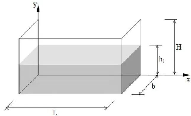
The SPH model described in this study was developed for rectangular liquid storage tanks with rigid walls subjected to horizontal earthquake ground motion. The model geometry is presented in Figure 1, where H, L and b represent the height, length and breadth of the liquid storage tank, respectively, whereas hl represents height of the liquid with a dynamic viscosity of μ and an initial density of ρ0. Each liquid particle is subjected to a
constant gravitational acceleration of g=9.81 m/s2 in -y direction and a horizontal earthquake ground acceleration, aG in x direction.
377 The equations describing the temporal variation of
density and acceleration are presented in Equations (1) and (2) using the principles of conservation of mass and the conservation of momentum.
Dρ Dt= -ρ∇u (1) Du Dt= -∇P+ μ ρ∇ 2u+f ρ (2)
where D/Dt is the material derivative, ρ is the fluid density, t is the time, u=(u,v) is the flow velocity vector, P is the absolute pressure and f is the body force vector, i.e. gravity(g), base excitation. Since the Lagrangian coordinates are being used, the velocity is expressed by Equation (3),
u=DxDt (3) where x=(x,y) denotes the position vector of the particle.
2.1 Kernel Function and Formulation
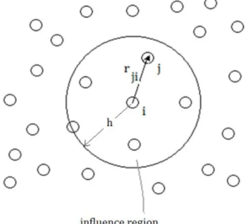
The physical variables are defined for each particle by a smooth, even, compact and unity Kernel function, W(r,h), where h is the smoothing distance, defining an influence region Ω, and r is the distance between particles (Figure 2). Kernel functions using the cubic polynomial and the Gauss distribution interpolation schemes are commonly used in Smoothed Particle Hydrodynamics applications. The selection of the Kernel function directly affects the accuracy and the stability of results. Derivations of various Kernel functions are explained in details in (Liu, 2003).
Figure 2. Particles where rji=rj - ri is the position vector from particle i to j.
In this study, Spiky Kernel (Desbrun, 1996) is used to overcome numerical challenges, i.e. clustering due
to collocative nature of the SPH method. For two dimensional geometries, the Spiky Kernel function is:
W(r,h)=α(h-r)3 for r<h (4) where α=10/πh5, h=max(h
x,hy) is the smoothing
length where hx=βL/Nx and hy=βhl/Ny are the
smoothing distances for the particles having a uniform initial distribution in x and y directions respectively. Nx and Ny are integers designating the
number of rows in x and y in turn. SPH requires necessary amount of particles in the smoothed region such that β=2 works well for such a two dimensional simulation. The integral form of the velocity function, u(r), smoothed over Ω, is expressed as:
𝐮(𝐫) = ∫ W(𝐫′, h)𝐮(𝐫′)d𝐫′
Ω (5)
and particle approximation of i is derived by summation in the smoothed region such that:
𝐮i= ∑ 𝐮jmj ρj Wij j (6) 𝛁𝐮i= ∑ 𝐮jmρj j 𝛁Wij j (7) 𝛁𝟐𝐮 i= ∑ 𝐮j mj ρj 𝛁 𝟐W ij j (8) where 𝐮i= 𝐮(𝐫i) , 𝐮j= 𝐮(𝐫j) and Wij= W(𝐫i−
𝐫j , h). Approximations of ρ and P are derived in a similar manner. Inserting the particle approximations of ρ, P and u into Navier-Stokes equations, leads to the discretized form of the equations of motion: Dρi Dt = ∑ m𝑗 j(𝐮i− 𝐮j)𝛁Wij (9) D𝐮i Dt = − ∑ mj( Pi ρi2+ Pj ρj2) 𝛁Wij 𝑗 + μi ρi∑ mj ρj(𝐮j− 𝐮i) 𝑗 𝛁𝟐Wij +ρ𝐟ii (10) D𝐱i Dt = 𝐮i (11) where 1 ≤ i ≤ NxNy and 1 ≤ j ≤ NxNy .
2.2 Pressure and Viscosity
The approximated form of the pressure term in (10) results in a system of symmetrical forces for each pair of particles. Since, it is quite difficult to approximate higher order derivate with the SPH Method in low resolution cases, viscous diffusion term is approximated with a first order derivation term in order to avoid using second order
Analysis of Seismic Sloshing Displacements in Rectangular Liquid Storage Tanks with SPH Method, Güray et.al.
378 derivation of the kernel function as proposed in
(Morris, 1997) which complies with the expression stated in (Monaghan, 1995). Rewriting the formula assuming that viscosity is constant for all particles leads to Equation (12): μi ρi∑ mj ρj(𝐮j− 𝐮i) j 𝛁𝟐Wij= 2μi ρi ∑ mj ρj 𝐫ij(𝐮i−𝐮j) (𝐫ij2+0.01h2) j 𝛁Wij (12)
Pressure is calculated for each particle with the Tait’s equation of state (Batchelor, 1974), widely employed in SPH formulations for nearly incompressible fluids with Equation (13),
Pi = B ((ρi
ρ0)
γ
− 1) (13)
where 𝐵 = 200𝜌0𝑔ℎ𝑙/𝛾 and 𝛾 = 7, keeping
density fluctuations at minimum, e.g. approximately 1 % (Monaghan, 2005).
2.3 Boundary Conditions
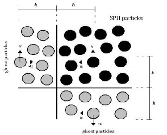
Wall boundaries are impenetrable solid boundaries and can be modeled with virtual particles. In this study, virtual/ghost particles are distributed out of the walls in the range of the smoothing distance, h (Figure 3). The information at ghost particles is assigned from the particles of the inner fluid domain. Each ghost particle has the same pressure and density with the corresponding inner fluid particle. Since the fluid does not penetrate through the solid walls, velocities normal to the wall are in opposite directions. Fluid is assumed to be inviscid such that velocities parallel to wall are in the same direction as outlined in Equation (14).
Pghost = Pinner ρghost= ρinner 𝐮ghostn = −𝐮 inner n 𝐮ghostt = 𝐮innert (14) where n and t are the normal and tangential directions, respectively. The free surface of the liquid was not subjected to constraints since pressure, density and velocities at the outer surface are used to obtain the updated geometry. In the case of resonance, where the pressure over the particles close to the wall, especially near the corners, is very high, it becomes inevitable to
prevent penetration of a particle through to the wall. In this study, the particles close to the side or bottom walls, are forced to bounce back when they are in a specific range of the distance to the wall such that their position remains the same but velocity vector normal to wall is redirected into the opposite direction and the speed is reduced by half due to inelastic collision at each new step (k + 1):
(𝐮n)(k+1)= e(𝐮n)(k) (15)
where e = 0.5 is the elastic collision constant.
Figure 3. Ghost particles behind solid walls.
2.4 Time scheduling
The equations 9 and 10 are discretized in time with 4th order Adams Bashford method (AB4). The
position (equation 11) is obtained by the Crank-Nicolson method. The main advantage of AB4 approach is that it does not require intermediate steps like the Runge Kutta or predictor-corrector methods. However, it is necessary to keep the old values of variables for such explicit methods. Rewriting the equations 9,10 and 11 after time integration results in equations 16, 17 and 18 at particle i: 𝐮i(k+1)= 𝐮i(k)+24∆t(55𝐅i(k)− 59𝐅i(k−1)+ 37𝐅i(k−2)− 9𝐅i(k−3)) (16) ρi(k+1)= ρi(k)+∆t 24(55𝐆i (k)− 59𝐆 i(k−1)+ 37𝐆i(k−2)− 9𝐆i(k−3)) (17) and 𝐱 i (k+1)= 𝐱 i (k)+∆t 2 (𝐮i (k+1)+ 𝐮 i (k)) (18)
379 here k denotes the time-step, ∆t = t(k+1)− t(k) and
𝐅i and 𝐆i are the right hand side of the equations 9
and 10, respectively.
3. Case Study and Discussion
Imperial Valley Earthquake (19.05.1940), El Centro Array 9, I-ELC180.AT2 acceleration time-history from the PEER NGA Strong Motion Database has been selected as the base excitation record for the experimental study (Figure 4). The record was scaled due to the limitations imposed by the shake table (Figure 5). Peak ground acceleration and the predominant period of the scaled earthquake ground motion record are 0.2457 g and 0.50s, respectively.
Figure 4. Base acceleration time-history record used in the study.
3.1 Experimental Analysis
The tank model (Figure 5) used in the experimental verification study has the dimensions 40 cm.,40 cm. and 30 cm. in height(H), width(L) and the breadth(b), respectively. Tank is filled with water with an initial density of ρ0=1000 kg/m3 up to a height of hl =10 cm. The water has been colored with red dye in order to facilitate image processing. The dynamical viscosity of the water is taken as μ=0.001 Pa·s. The liquid tank is made of Plexiglas panels with a thickness of 1 cm and is firmly fixed to the shake table with bolts. Free surface sloshing displacements were recorded with a high resolution video camera throughout the experiment.
Figure 5. Experimental setup.
3.2 Flow Modeling Software
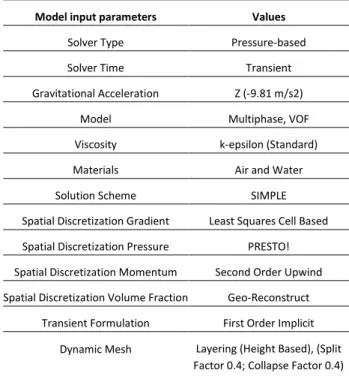
In addition to the experimental study, flow modeling software (Ansys Fluent v14.5) is used to obtain numerical results with a mesh-using method. Geometric model of the rectangular liquid tank was created with Ansys Design Modeler and meshed using 480000 quadratic elements with the meshing module of Ansys. The top boundary surface of the geometric model was specified as a “pressure outlet” while the rest of the boundary surface was specified as “walls”. Afterwards, the finite element mesh of the liquid storage tank with the specified boundary conditions was transferred to the Ansys Fluent CFD module. The effect of earthquake base excitation was simulated by moving the walls and the interior body with user defined functions. Fluent model input options, used in the study are outlined in Table 1.
Table 1. Ansys Fluent model input parameters Model input parameters Values
Solver Type Pressure-based
Solver Time Transient
Gravitational Acceleration Z (-9.81 m/s2)
Model Multiphase, VOF
Viscosity k-epsilon (Standard)
Materials Air and Water
Solution Scheme SIMPLE
Spatial Discretization Gradient Least Squares Cell Based Spatial Discretization Pressure PRESTO! Spatial Discretization Momentum Second Order Upwind Spatial Discretization Volume Fraction Geo-Reconstruct
Transient Formulation First Order Implicit Dynamic Mesh Layering (Height Based), (Split
Analysis of Seismic Sloshing Displacements in Rectangular Liquid Storage Tanks with SPH Method, Güray, Yazıcı, Aksel
380
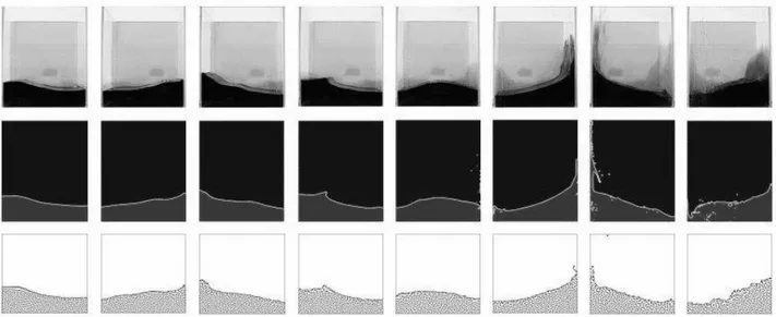
Figure 6. Sloshing snopshots at t=24.235, 24.710, 24.970, 25.190, 25.790, 26.510, 28.825, 29.260 sec.’s from left to right. Experimental study, Fluent analysis solution and the SPH method solution from top to bottom.
3.3 SPH Simulation
Numerical testing using the SPH method is conducted with 60x15=900 particles assuming a 2D tank geometry. The particles are initially distributed with a uniform spacing of ∆x=L/60=hl /15 from
center to center. The time step is selected as ∆t=5x10⁻⁵ which is sufficiently small to satisfy the
time stability conditions. Since the time step interval of the original acceleration time history record was larger, the selected time step for the analysis, intermediate acceleration values were obtained using linear interpolation.
The boundary line above the particles in the SPH model analysis results shows the free surface tracking. This line is predicted by marking the zero crossings of the Laplacian of the density. Since the zero Laplacian passes above the free surface, a threshold value of δ which is greater than zero is used to find the approximate location of this line.
|∇2ρ| ≤ δ (19)
The free surface displacement profiles at 8 different instances are presented in the Figure 6, where the first, second and third row of snapshots show the results obtained from the experimental study, the flow modelling software and the SPH model, respectively. The results obtained from the SPH model strongly agree with the results obtained from the experiment and a flow modelling software using finite elements method.
4. Conclusions
Smoothed Particle Hydrodynamics (SPH) is an efficient method to simulate free surface flows. Computations are performed on a personal computer equipped with an AMD Athlon X2 Dual Core processor. SPH code is verified with an experiment and the results of the Ansys Fluent software. Only 900 number of SPH particles are used and the values of variables are not corrected as in the case of XSPH (Monaghan, 1989). Even to this fact, the comparable instants from both experiment and the Ansys model show that the SPH method is highly capable of not only capturing basic sloshing wave patterns but also simulating more complicated subordinate sloshing waves. High resolution is necessary for more realistic drifting on the side walls. Time stepping is chosen according to Courant condition such that denser particles will require less time-stepping.
Bibliography
Batchelor, G.K., 1974. An Introduction to Fluid Mechanics, 4th. Edn. Cambridge University Press, Cambridge.
Bulian, G, Cercos-Pita, J.L. 2018. Co-simulation of ship motions and sloshing in tanks, Ocean Engineering, 152:353–376
Crespo, A.J.C., 2008. Application of the Smoothed Particle Hydrodynamics Model SPHysics to Freesurface Hydrodynamics, PhD Thesis, Tese de doutorado, Universidade de Vigo, Espanha.
381 Chen, J.Y, Lien, F.S., 2018, Simulations for soil explosion
and its effects on structures using SPH method,
International Journal of Impact Engineering, 112:
41-51.
Desbrun, M., Gascuel, M.P., 1996, Smoothed Particles: A new paradigm for animating highly deformable bodies, Proceedings of Eurographics Workshop on
Computer Animation and Simulation ‘96, pp. 61-76,
Springer.
El Damatty A.A., Sweedan A.M.I., 2006, Equivalent mechanical analog for dynamic analysis of pure conical tanks, Thin Walled Structures, 44: 429-440.
Frandsen, J.B., 2004, Sloshing motions in excited tanks,
Journal of Computational Physics, 196:53-87
Gingold, R.A., Monaghan, J.J., 1977, Smoothed particle hydrodynamics: Theory and application to the non-spherical stars, Mon. Not. R. Astron. Soc.,181:375-389.
Graham, E.W., Rodriguez, A.M., 1952,The characteristics of fuel motion which affect the motion of the airplane dynamics, Applied Mechanics,19: 381-388.
Hanson, R.D., 1973, Behavior of Liquid Storage Tanks, The Great Alaska Earthquake of 1964, National Academy
of Science, Washington D.C.,7:331-339.
Haroun, M.A., Housner, G.W., 1981, Seismic Design of Liquid-Storage Tanks, Journal of Technical Councils,
ASCE, 107: 191-207.
Housner, G.W., 1963, The dynamic behaviour of water tanks, Bulletin of the Seismological Society of America, 53: 381-387.
Khanpour, M., Zarrati, A.R., Kolahdoozan, M., Shakibaeinia , A., Amirshahi, S.M., 2016, Mesh-Free SPH Modeling of Sediment Scouring and Flushing,
Computers and Fluids, 129: 67–78.
Liu, G.R., Liu, M.B., 2003, Smoothed Particle Hydrodynamics, a meshfree particle method, 59-101,
World Scientific Publishing Co. Pte.Ltd., Singapore.
Lucy, L.B., 1977, A numerical approach to the testing of the fission hypothesis, Astron. J., 83: 1013-1024.
Monaghan, J.J., 1989, On the Problem of Penetration in Particle Methods, Journal of Computational Physics, 82(1): 1–15.
Monaghan, J.J., 1995, Heat Conduction with discontinuous conductivity, Applied Mathematics
Reports and Preprints 95/18, Monash University,
Melbourne, Australia.
Monaghan,J.J., 2005, Smoothed Particle Hydrodynamics,
Rep. Prog. Phys., 68: 1703-1759.
Morris, J.P., Fox, P.J., Zhu, Y., 1997, Modeling Low Reynolds Number Incompressible Flows Using SPH,
Journal of Computational Physics, 136: 214-226.
Nakayama, T., Washizu, K., 1981, The Boundary Element Method Applied to The Analysis of Two-Dimensional Nonlinear Sloshing Problems, International Journal
For Numerical Methods in Engineering, 17:
1631-1646.
Sames, P.C., Marcouly, D., Schellin, T.E., 2002, Sloshing in rectangular and cylindrical tanks, J. Ship Res., 46:186-200.
Steinbrugge, K.V., Rodrigo, F.A., 1963, The Chilean Earthquakes of May 1960: A Structural Engineering Viewpoint, Bulletin of the Seismological Society of
America, 53: 225-307.
Vignjevic, R., Campbell, J., 2009, Review of the development of the smooth particle hydrodynamics (SPH) method, in S.Hiermaier, editor, Predictive modeling of dynamic processes, 367-396, Springer, Dordrecht Heidelberg London New York.
Wang, L., Wang, Z., Li, Y., 2013, A SPH simulation on large-amplitude sloshing for fluids in a two-dimensional tank, Earthq Eng & Eng Vib, 12: 135-142.
Wu, G.X., Ma, Q.W., Taylor, R.E., 1998, Numerical simulation of sloshing waves in a 3D tank based on a finite element method, Appl. Ocean Res., 20: 337-355.