The Milne problem using the PN method for a nonabsorbing medium with linearly anisotropic scattering

c

⃝ T¨UB˙ITAK

doi:10.3906/fiz-1610-26 h t t p : / / j o u r n a l s . t u b i t a k . g o v . t r / p h y s i c s /

Research Article

The Milne problem using the P

method for a nonabsorbing medium with

linearly anisotropic scattering

Mustafa C¸ etin G ¨ULEC¸ Y ¨UZ1,∗, Ahmet ERSOY1,2

1

Department of Physics, Ankara University, Ankara, Turkey

2_{Department of Physics, Karamano˘glu Mehmetbey University, Karaman, Turkey}

Received: 25.10.2016 • Accepted/Published Online: 04.01.2017 • Final Version: 05.09.2017

Abstract: The Milne problem, known as one of the classical problems of radiative transfer and neutron transport theory,

is solved using the PN method for a nonabsorbing medium (c = 1) with a linearly anisotropic scattering kernel. Specular and diffuse reflection boundary conditions are taken into account. The numerical results are listed for different selected parameters. Some results are also compared with the literature.

Key words: PN method, Milne problem, extrapolated endpoint, nonabsorbing medium, specular and diffuse reflectivity, anisotropic scattering

1. Introduction

The Milne problem is a well-known problem in both the radiative transfer field and neutron transport theory [1]. In this problem, the angular distribution of the flux due to monoenergetic neutrons or radiations diffusing from a source at infinity (x > 0) can be obtained in a source-free half-space (x < 0) [2,3].

In this paper the effect of linearly anisotropic scattering with specular and diffuse reflecting boundaries on the extrapolated endpoint z0 for the Milne problem is studied in a nonabsorbing medium using Legendre

polynomial approximation. Numerical results for z0 and the emergent angular distribution Ψ(0,−µ) are given

and compared with the literature.

In the plane geometry, the one-speed, time-independent neutron transport equation for linearly anisotropic scattering is [4] µ∂Ψ(x, µ) ∂x +Ψ (x, µ) = c 2 +1 ∫ −1 (1 + 3f1µµ ′ )Ψ ( x,µ′ ) dµ′ (1)

where Ψ (x, µ) is the angular distribution of neutrons, c is the number of secondary neutrons per collision, µ is the cosine of the angle between the direction of the neutron velocity and the positive x axis, and 3f1 (–1 ≤

3f1≤ +1) is the coefficient of the linearly anisotropic scattering.

The Milne problem will be solved with the following boundary conditions [5]:

Ψ (0, µ) =ρsΨ (0,−µ) +2ρd +1 ∫ −1 µ′Ψ ( 0,µ′ ) dµ′, µ > 0 (2) ∗_{Correspondence: gulecyuz@science.ankara.edu.tr}

and

lim

x→∞Ψ (x, µ) = 0, (3)

where ρs_(0≤ρs_{≤ 1) and ρ}d_(0≤ρd_{≤ 1) are the specular and diffuse reflectivity of the boundary, respectively.}

2. Method and calculation

In the PN method, by using the expansion of the angular distribution in terms of Legendre polynomials [6],

Ψ (x, µ) = ∞ ∑ n=0 2n + 1 2 Ψn(x) Pn(µ) (4)

and multiplying both sides of Eq. (1) by Pm(µ) , then integrating over µ in an interval [–1, +1] and using the orthogonality of the Legendre polynomials leads to the following moment equations, which consist of the infinite sets of coupled differential equations with m = 0,1,...,N [7], [8]:

mdΨm−1(x) dx + (m + 1) dΨm+1(x) dx + (2m + 1) [1− c (δm0− f1δm1)] Ψm(x) = 0 (5) Here +1 ∫ −1 Pn(µ)Pm(µ)dµ = 2 2m + 1δnm, (6) µPm(µ) = 1 2m + 1[(2m + 1) Pm+1(µ) +mPm−1(µ)] . (7)

In order to solve Eq. (5) it is sufficient to get dΨm+1(x)/dx = 0 . As a result of this, N + 1 equations that consist of N + 1 unknowns are obtained.

P1 approximation: In P1 approximation for nonabsorbing medium i.e. c = 1, the moment equations

from Eq. (5) are

dΨ1(x)

dx = 0, (8a)

dΨ0(x)

dx +3 (1−f1) Ψ1(x) = 0. (8b)

Ψ1(x) is a constant as seen in Eq. (8a) and so assuming Ψ1(x) =−1 and then substituting it in Eq. (8b) we

get

Ψ0(x) = 3 (1−f1) x+A0 (9)

and from Eq. (4)

Ψ (0, µ) =1

2Ψ0(0) P0(µ) + 3

2Ψ1(0) P1(µ) , (10)

where A0 is constant and can be obtained using the Marshak boundary condition given by [9], +1

∫ −1

Using Eq. (2), we can rewrite the Marshak boundary condition as 1 ∫ 0 µmΨ(0, µ)dµ−ρs 1 ∫ 0 µmΨ (0,−µ) dµ− 2ρ d m + 1 1 ∫ 0 µ′Ψ ( 0,µ′ ) dµ′= 0, m = 1, 3, ..., N (12)

Then A0 can be obtained as

A0= 2

1+ρs_+ρd

1−ρs−ρd, (13)

The extrapolated endpoint z0is defined as a distance from a vacuum boundary to where the asymptotic intensity

vanishes and it can be written mathematically as Ψ0(−z0) = 0 . From the definitions one can get

z0=

A0

3(1−f1)

(14)

P3 approximation: In P3 approximation the moment equations from Eq. (5) can be written as

dΨ1(x) dx = 0, (15a) 2dΨ2(x) dx + dΨ0(x) dx +3 (1−f1) Ψ1(x) = 0, (15b) 3dΨ3(x) dx +2 dΨ1(x) dx +5Ψ2(x) = 0, (15c) 3dΨ2(x) dx +7Ψ3(x) = 0. (15d)

From Eq. (15c) and Eq. (15d), a differential equation for Ψ2(x) is

−9

7

d2Ψ2(x)

dx2 +5Ψ2(x) = 0 (16)

and the solution of this equation is given by

Ψ2(x) =A1exp (−α1x) ; α1= ( 35 9 )1 2 (17)

where A1 is constant. Inserting Eq. (17) into Eq. (15d), Ψ3(x) can be written as

Ψ3(x) =

3

7A1α1exp (−α1x) (18)

Using Eqs. (17) and (18) and Ψ1(x) =−1 in Eq. (15b)

is obtained. Here A0 is constant and from Eq. (4) we get Ψ (0, µ) =1 2Ψ0(0) P0(µ) + 3 2Ψ1(0) P1(µ) + 5 2Ψ2(0) P2(µ) + 7 2Ψ3(0) P3(µ) (20)

The lowest order of Marshak boundary conditions given in Eq. (12) and Eq. (20) are used to determine A0

and A1 constants A0=−2− 4 ρs_ρd−1+ 42(1+ρs) 175(ρs−1) + 96α 1(1+ρs) , (21a) A1= 56(1+ρs) 175(ρs−1) + 96α 1(1+ρs) . (21b)

Finally, the extrapolated endpoint z0 is calculated from Eq. (14) using A0 in Eq. (21a) for P3 approximation.

P5 approximation: In P5 approximation the moment equations are obtained from Eq. (5)

dΨ1(x) dx = 0, (22a) 2dΨ2(x) dx + dΨ0(x) dx +3 (1−f1) Ψ1(x) = 0, (22b) 3dΨ3(x) dx +2 dΨ1(x) dx +5Ψ2(x) = 0, (22c) 4dΨ4(x) dx +3 dΨ2(x) dx +7Ψ3(x) = 0, (22d) 5dΨ5(x) dx +4 dΨ3(x) dx +9Ψ4(x) = 0, (22e) 5dΨ4(x) dx +11Ψ5(x) = 0. (22f)

After some algebraic manipulations in Eqs. (22), a differential equation is found as follows: 44 77 d4_Ψ 4(x) dx4 − 378 55 d2_Ψ 4(x) dx2 +9Ψ4(x) = 0, (23)

and the solution of this equation is

Ψ4(x) =A1exp (−α1x) +A2exp (−α2x) (24)

Ψ5(x) can be derived from Eq. (22f)

Ψ5(x) =

−5

11

dΨ4(x)

dx (25)

and the other solutions of moment equations can be found as

Ψ3(x) =− ∫ 9 4 ( Ψ4(x) + 5 9 dΨ5(x) dx ) dx,

Ψ2(x) =− ∫ 7 3 ( Ψ3(x) + 4 7 dΨ4(x) dx ) dx, Ψ1(x) =−1, Ψ0(x) =−3 ∫ [ (1−f1) Ψ1(x) + 2 3 dΨ2(x) dx ] dx+A0. (26)

A0, A1, A2 are constants and can be calculated by using Marshak boundary conditions given in Eq. (12) and

from Eq.(4) we obtained Ψ (0, µ) =1 2Ψ0(0) P0(µ) + 3 2Ψ1(0) P1(µ) + 5 2Ψ2(0) P2(µ) + 7 2Ψ3(0) P3(µ) +9 2Ψ4(0) P4(µ) + 11 2 Ψ5(0) P5(µ) (27)

As a result, we can generalize the moment equations for PN approximation as dΨ1(x) dx = 0, 2dΨ2(x) dx + dΨ0(x) dx +3 (1−f1) Ψ1(x) = 0, 3dΨ3(x) dx +2 dΨ1(x) dx +5Ψ2(x) = 0, · · · NdΨN(x) dx + (N− 1) dΨN−2(x) dx + (2N− 1) ΨN−1(x) = 0, NdΨN−1(x) dx + (2N + 1) ΨN(x) = 0, (28)

and the solutions of these equations are

ΨN−1(x) = N−1 2 ∑ k=1 Akexp(−αkx), ΨN(x) = −N 2N + 1 dΨN−1(x) dx , Ψk−2(x) =− ∫ 2k− 1 k− 1 ( Ψk−1(x) + k 2k− 1 dΨk(x) dx ) dx, k = 4, 5, ..., N Ψ1(x) =−1, Ψ0(x) =−3 ∫ [ (1−f1) Ψ1(x) + 2 3 dΨ2(x) dx ] dx+A0, (29)

The A0 and Ak constants can be determined by Eq. (12) and the extrapolated endpoint is calculated from Eq. (14).

3. Results

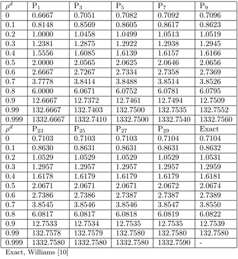
Numerical values of the extrapolated endpoint are given in isotropic scattering for diffuse and specular reflection in Tables 1 and 2, respectively. They are compared with the exact values in Williams’s paper [10]. Table 3 shows the extrapolated endpoints for different values of ρs _{and ρ}d _{in isotropic scattering. These results are} compared with Degheidy [11]. It can be seen from these tables that z0, the distance at which the flux drops

to zero, increases with increasing specular and diffuse components of reflectivity. In Tables 4 and 5, numerical values of z0 are given for different values of ρs and ρd in linearly anisotropic scattering compared with Atalay

[12,13]. In these tables, the extrapolated endpoint values increase with increasing linearly anisotropic scattering function. Table 6 shows the emergent angular distribution Ψ(0,−µ) for various values of ρs and ρd in isotropic scattering (f1 = 0). In all our computations, we used Mathematica programming.

Table 1. The extrapolated endpoint for diffuse reflection ( ρs _{= 0) and isotropic scattering (f} 1 = 0). ρd P1 P3 P5 P7 P9 0 0.6667 0.7051 0.7082 0.7092 0.7096 0.1 0.8148 0.8532 0.8564 0.8573 0.8578 0.2 1.0000 1.0338 1.0415 1.0425 1.0430 0.3 1.2381 1.2765 1.2796 1.2806 1.2810 0.4 1.5556 1.5940 1.5971 1.5981 1.5985 0.5 2.0000 2.0384 2.0415 2.0425 2.0430 0.6 2.6667 2.7051 2.7082 2.7092 2.7096 0.7 3.7778 3.8162 3.8193 3.8203 3.8208 0.8 6.0000 6.0384 6.0415 6.0425 6.0430 0.9 12.6667 12.7051 12.7082 12.7092 12.7096 0.99 132.6670 132.7051 132.7082 132.7092 132.7097 0.999 1332.6700 1332.7050 1332.7080 1332.7090 1332.7090 ρd P23 P25 P27 P29 Exact 0 0.7103 0.7103 0.7103 0.7104 0.7104 0.1 0.8585 0.8585 0.8585 0.8585 0.8585 0.2 1.0437 1.0437 1.0437 1.0437 1.0437 0.3 1.2817 1.2818 1.2818 1.2818 1.2818 0.4 1.5992 1.5992 1.5992 1.5992 1.5993 0.5 2.0436 2.0437 2.0437 2.0437 2.0437 0.6 2.7103 2.7103 2.7103 2.7104 2.7104 0.7 3.8214 3.8214 3.8215 3.8215 3.8214 0.8 6.0436 6.0437 6.0437 6.0437 6.0436 0.9 12.7103 12.7103 12.7103 12.7104 12.7104 0.99 132.7103 132.7103 132.7103 132.7104 -0.999 1332.7100 1332.7100 1332.7100 1332.7100 -Exact, Williams [10] 4. Discussion

The Milne problem with specular and diffuse reflecting boundary conditions is solved using Legendre polynomial approximation, which is known as the PN method. Extrapolated endpoint z0 is the distance from the boundary

to where the asymptotic component of density goes to zero. It was calculated for the nonabsorbing medium where the average number of secondary neutrons per collision equals unity. There are only scattering collisions

with no neutron loss. Furthermore, the linearly anisotropic scattering function is considered. For Nth order approximation, N + 1 set of coupled differential equations are defined and reduced to one (N – 1)th order differential equation for ΨN₋₁(x) in the PN method. The remaining N moments for ΨN(x) are derived after writing the solution of ΨN−1(x). The constants of these solutions are calculated using Marshak boundary conditions with specular and diffuse reflectivity of the boundary. Then z0 is obtained using the A0 constant

for each Nth order approximation. Some of our results are compared with the literature and these results are in agreement.

Table 2. The extrapolated endpoint for specular reflection ( ρd = 0) and anisotropic scattering (f1 = 0).

ρd P1 P3 P5 P7 P9 0 0.6667 0.7051 0.7082 0.7092 0.7096 0.1 0.8148 0.8569 0.8605 0.8617 0.8623 0.2 1.0000 1.0458 1.0499 1.0513 1.0519 0.3 1.2381 1.2875 1.2922 1.2938 1.2945 0.4 1.5556 1.6085 1.6139 1.6157 1.6166 0.5 2.0000 2.0565 2.0625 2.0646 2.0656 0.6 2.6667 2.7267 2.7334 2.7358 2.7369 0.7 3.7778 3.8414 3.8488 3.8514 3.8526 0.8 6.0000 6.0671 6.0752 6.0781 6.0795 0.9 12.6667 12.7372 12.7461 12.7494 12.7509 0.99 132.6667 132.7403 132.7500 132.7535 132.7552 0.999 1332.6667 1332.7410 1332.7500 1332.7540 1332.7560 ρd P23 P25 P27 P29 Exact 0 0.7103 0.7103 0.7103 0.7104 0.7104 0.1 0.8630 0.8631 0.8631 0.8631 0.8632 0.2 1.0529 1.0529 1.0529 1.0529 1.0531 0.3 1.2957 1.2957 1.2957 1.2957 1.2959 0.4 1.6178 1.6179 1.6179 1.6179 1.6181 0.5 2.0671 2.0671 2.0671 2.0672 2.0674 0.6 2.7386 2.7386 2.7387 2.7387 2.7389 0.7 3.8545 3.8546 3.8546 3.8547 3.8550 0.8 6.0817 6.0817 6.0818 6.0819 6.0822 0.9 12.7533 12.7534 12.7535 12.7535 12.7539 0.99 132.7578 132.7579 132.7580 132.7580 132.7580 0.999 1332.7580 1332.7580 1332.7580 1332.7590 -Exact, Williams [10]

Table 3. The extrapolated endpoint for different values of ρs_{, ρ}d_{, and isotropic scattering case (f}

1 = 0) in P29 approximation. ρs _{/ ρ}d 0.1 0.2 0.3 0.4 A B A B A B A B 0.1 1.0483 1.0484 1.2910 1.2912 1.6132 1.6133 2.0624 2.0626 0.2 1.2864 1.2865 1.6085 1.6086 2.0576 2.0578 2.7291 2.7292 0.3 1.6039 1.6039 2.0529 2.0531 2.7243 2.7245 3.8402 3.8453 0.4 2.0483 2.0484 2.7196 2.7197 3.8354 3.8356 6.0624 6.0626

Table 4. The extrapolated endpoint for specular and diffuse reflection in linearly anisotropic scattering for P29 approximation. ρd _{or ρ}s f1= 0.1 Diffuse Specular A B A B 0 0.7893 0.7894 0.7893 0.7894 0.1 0.9539 0.9568 0.9590 0.9592 0.2 1.1597 1.1660 1.1699 1.1702 0.3 1.4242 - 1.4397 -0.4 1.7769 - 1.7977 -0.5 2.2708 2.2959 2.2969 2.2989 0.6 3.0115 - 3.0430 -0.7 4.2461 - 4.2830 -0.8 6.7152 - 6.7576 -0.9 14.1226 14.3479 14.1706 14.2089 0.99 147.4560 149.9330 147.5089 147.9930 0.999 1480.7893 - 1480.8430 -ρd _{or ρ}s f1= 0.2 Diffuse Specular A B A B 0 0.8879 0.8881 0.8879 0.8881 0.1 1.0731 1.0764 1.0789 1.0791 0.2 1.3046 1.3118 1.3162 1.3165 0.3 1.6022 - 1.6197 -0.4 1.9991 - 2.0224 -0.5 2.5546 2.5283 2.5840 2.5863 0.6 3.3879 - 3.4234 -0.7 4.7768 - 4.8184 -0.8 7.5546 - 7.6023 -0.9 15.8879 16.1414 15.9419 15.9850 0.99 165.8879 168.6740 165.9476 166.4920 0.999 1665.8879 - 1665.9480 -ρd or ρs f1= 0.3 Diffuse Specular A B A B 0 1.0148 1.0149 1.0148 1.0149 0.1 1.2264 1.2301 1.2330 1.2332 0.2 1.4910 1.4992 1.5042 1.5046 0.3 1.8311 - 1.8511 -0.4 2.2846 - 2.3113 -0.5 2.9196 2.9519 2.9531 2.9557 0.6 3.8719 - 3.9124 -0.7 5.4592 - 5.5067 -0.8 8.6338 - 8.6884 -0.9 18.1577 18.4473 18.2193 18.2686 0.99 189.5862 192.7710 189.6543 190.2770 0.999 1903.8719 - 1903.9410

Table 5. The extrapolated endpoint for different values of ρs and ρd in linearly anisotropic scattering (f1̸= 0) for P29 approximation. f1 = 0.1 ρs / ρd 0.1 0.2 0.3 0.4 0.5 0.1 1.16475 1.43446 1.79241 2.29151 3.03757 0.2 1.42930 1.78720 2.28624 3.03225 4.27213 0.3 1.78203 2.28102 3.02698 4.26681 6.74127 0.4 2.27586 3.02176 4.26155 6.73595 14.14871 0.5 3.01662 4.25636 6.73071 14.14339 -f1 = 0.2 ρs / ρd 0.1 0.2 0.3 0.4 0.5 0.1 1.31034 1.61377 2.01646 2.57794 3.41726 0.2 1.60796 2.01060 2.57202 3.41128 4.80615 0.3 2.00479 2.56615 3.40535 4.80017 7.58393 0.4 2.56034 3.39949 4.79424 7.57794 15.91730 0.5 3.39370 4.78840 7.57205 15.91131 -f1 = 0.3 ρs _{/ ρ}d _{0.1 0.2 0.3 0.4 0.5} 0.1 1.49754 1.84431 2.30453 2.94622 3.90544 0.2 1.83767 2.29782 2.93945 3.89860 5.49274 0.3 2.29119 2.93275 3.89183 5.48590 8.66735 0.4 2.92611 3.88513 5.47913 8.66051 18.19120 0.5 3.87851 5.47246 8.65377 18.18436

-Table 6. The emergent angular distribution Ψ(0,−µ) for selected values of ρs _{and ρ}d _{in isotropic scattering (f} 1 = 0). ρs_{= 0} –µ ρd _{= 0.0 ρ}d _{= 0.2 ρ}d _{= 0.4 ρ}d _{= 0.6 ρ}d _{= 0.8} 0.1 1.18027 1.68027 2.51360 4.18027 9.18027 0.2 1.19913 1.69913 2.53246 4.19913 9.19913 0.3 1.46110 1.96110 2.79444 4.46110 9.46110 0.4 1.55339 2.05339 2.88673 4.55339 9.55339 0.5 1.76704 2.26704 3.10037 4.76704 9.76704 0.6 1.88438 2.38438 3.21771 4.88438 9.88438 0.7 2.05383 2.55383 3.38717 5.05383 10.05380 0.8 2.22933 2.72933 3.56266 5.22933 10.22930 0.9 2.38267 2.88267 3.71600 5.38267 10.38270 1.0 2.59895 3.09895 3.93228 5.59895 10.59890 ρd = 0 - µ ρs_{= 0.0 ρ}s _{= 0.2 ρ}s _{= 0.4 ρ}s_{= 0.6 ρ}s_{= 0.8} 0.1 1.18027 1.68504 2.50759 4.19368 9.38526 0.2 1.19913 1.67880 2.57907 4.13763 9.07603 0.3 1.46110 1.96261 2.78528 4.46511 9.59919 0.4 1.55339 2.04421 2.93737 4.52577 9.48316 0.5 1.76704 2.27007 3.09607 4.77591 9.88266 0.6 1.88438 2.38146 3.26017 4.87573 9.86080 0.7 2.05383 2.55470 3.41334 5.05653 10.08230 0.8 2.22933 2.73506 3.55956 5.24654 10.34169 0.9 2.38267 2.88912 3.71281 5.40209 10.49565 1.0 2.59895 3.11776 3.82831 5.65495 10.97911

References [1] Placzek, G.; Seidel, W. Phys. Rev. 1947, 72, 550-555.

[2] Razi, N. K. J. Quant. Spectrosc. Radiat. Transf. 1993, 50, 59-64.

[3] Abdel-Krim, M. S., Degheidy, A. R. Ann. Nucl. Energy 1998, 25, 317-325.

[4] Case, K. M.; Zweifel, P. E. Linear Transport Theory, Addison-Wesley: London, UK, 1967. [5] Marshak, R. E. Phys. Rev. 1947, 71, 688-693.

[6] Erdogan, F., Tezcan, C. J. Quant. Spectrosc. Radiat. Transf. 1995, 53, 681-686.

[7] McCormick, N. J. PhD, Department of Physics, University of Michigan, Ann Arbor, MI, USA, 1964. [8] McCormick, N. J., Kuscer, I. J. J. Math. Phys. 1965, 6, 1939-1945.

[9] Marshak, R. E. Phys. Rev. 1947, 71, 443-446.

[10] Williams, M. M. R. Atom Kern Energie 1975, 25, 19-25.

[11] Degheidy, A. R., El-Shahat, A. Ann. Nucl. Energy 2010, 37, 1443-1446.

[12] Atalay, M. A. J. Quant. Spectrosc. Radiat. Transf. 2002, 72, 589-606.