ESTIMATING CONSUMER SURPLUS IN EBAY COMPUTER MONITOR AUCTIONS A Master’s Thesis by TUĞBA GİRAY Department of Economics Bilkent University Ankara January 2006
ESTIMATING CONSUMER SURPLUS IN EBAY COMPUTER MONITOR AUCTIONS
The Institute of Economics and Social Sciences of
Bilkent University
by
TUĞBA GİRAY
In Partial Fulfilment of the Requirements for the Degree of MASTER OF ARTS
in
THE DEPARTMENT OF ECONOMICS BİLKENT UNIVERSITY
ANKARA January 2006
I certify that I have read this thesis and have found that it is fully adequate, in scope and in quality, as a thesis for the degree of Master of Arts in Economics.
Asst. Prof. Kevin Hasker Supervisor
I certify that I have read this thesis and have found that it is fully adequate, in scope and in quality, as a thesis for the degree of Master of Arts in Economics.
Asst. Prof. Taner Yiğit
Examining Committee Member
I certify that I have read this thesis and have found that it is fully adequate, in scope and in quality, as a thesis for the degree of Master of Arts in Economics.
Assoc. Prof. Süheyla Özyıldırım Examining Committee Member
Approval of the Institute of Economics and Social Sciences
Prof. Dr. Erdal Erel Director
ABSTRACT
ESTIMATING CONSUMER SURPLUS IN eBay COMPUTER MONITOR AUCTIONS
Giray, Tuğba
M.A., Department of Economics Supervisor: Asst. Prof. Kevin Hasker
January 2006
In this study, using data from computer monitor auctions on eBay collected in 2000, bidding functions are estimated by maximum likelihood using five different assumptions about the underlying distribution of independent private values. It is assumed that these values come from the logistic, gamma, weibull, pareto and lognormal distributions. Next, consumer surplus in the market for computer monitors is estimated and its sensitivity to different distributional specifications is tested. Two types of consumer surplus estimates are provided. First, ex-post consumer surplus estimates are constructed and then a lower bound for consumer surplus is computed using a “rational reassignment” methodology. Median consumer surplus estimates vary from $39 with the logistic to $143 with the lognormal, or the consumers’ share of surplus from 30% to 61%. Expected consumer surplus estimates indicate a high sensitivity to the distribution specification, especially to the tails of the distribution. Lower bound estimates are more solid and more reliable since they are independent of the tails. Accordingly, these statistics, which do not vary with distribution, yield a
median estimate of $41 and a consumer share of 32%. Finally, the last part of this study examines which distribution best fits the data. Information criteria favor the gamma distribution, tests against the empirical distribution of second and third highest values prefer the logistic distribution.
ÖZET
eBay BİLGİSAYAR MONİTORÜ MARKETİNDE TÜKETİCİ FAZLASININ TAHMİNİ
Giray, Tuğba
Yüksek Lisans, İktisat Bölümü Tez Yöneticisi: Yrd. Doç. Dr. Kevin Hasker
Ocak 2006
Bu çalışmada, fiyat teklifi fonksiyonları en büyük olabilirlik kestirimi tekniği ile, bağımsız özel değerlerin temelindeki dağılım hakkında beş farklı varsayıma dayanılarak ve eBay bilgisayar monitorü açık artırmalarından 2000 yılında toplanan data kullanılarak tahmin edilmektedir. Bu değerlerin, sırasıyla, lojistik, gamma, weibull, pareto ve lognormal dağılımlarından geldiği varsayılmaktadır. Sonrasında, bilgisayar monitörü marketindeki tüketici fazlası tahmin edilmekte ve değişik dağılım tayinlerine karşı duyarlılığı test edilmektedir. İki tür tüketici fazlası tahmini sağlanmaktadır. İlk önce, gerçekleşen tüketici fazlası tahminleri yaratılmakta ve sonrasında tüketici fazlası için bir alt sınır tahmini “mantıksal yeniden atama” yöntemi ile hesaplanmaktadır. Medyan tüketici fazlası tahminleri lojistik dağılımla $39 ile lognormal dağılımla $143 arasında değişmekte, ya da başka bir deyimle, tüketicilerin fazladaki payı %30 ile %61 arasında kalmaktadır. Beklenen tüketici fazlası tahminleri dağılım tayinine, özellikle dağılımın kuyruklarına, yüksek hassasiyete işaret etmektedir. Alt sınır tahminleri dağılımın kuyruklarından bağımsız
olduğu için daha sağlam ve güvenilirdir. Dolayısıyla, dağılıma göre değişmeyen bu istatistikler $41 medyan tüketici fazlası ve %32 tüketici payı tahminleri sunmaktadır. Son olarak, hangi dağılımın dataya en iyi uyduğu incelenmektedir. Bilgi kriterleri gamma dağılımını, ikinci ve üçüncü en yüksek değerlerin ampirik dağılımına karşı yapılan testler lojistik dağılımı tercih etmektedir.
TABLE OF CONTENTS
ABSTRACT...iii
ÖZET ... v
TABLE OF CONTENTS ...vii
LIST OF TABLES………...viii
LIST OF FIGURES……….ix
CHAPTER 1…...1
CHAPTER 2...4
2.1 Literature Review...4
2.2 Data Set and Collection Techniques ………..6
2.3 The Model and Likelihood Functions ………8
2.4 The Distributions ……….12
2.5 The Estimates ………...13
CHAPTER 3...23
3.1 Consumer Surplus...23
3.2 Consumer Share………25
3.3 Lower Bound Estimates………26
CHAPTER 4...28
4.1 Tests Based on the Log-Likelihood………..29
4.2 Tests Against the Empirical Distribution of Values……….31
4.2.1 An Out of Sample Second Highest Values Test ………32
4.2.2 A Third Highest Values Test……….. 34
4.3 Comparing the Distribution of Second Highest and Third Highest Bids….38 CHAPTER 5………...39
SELECT BIBLIOGRAPHY………...43
LIST OF TABLES
1. Table 1: Estimates of the Exogenous Value of a Monitor……….14
2. Table 2: Log of Predicted Exogenous Values….………...15
3. Table 3: Estimates of the Entry Process……….18
4. Table 4: Predicted Values for the Log of Entry Parameter………21
5. Table 5: Expected Consumer Surplus………25
6. Table 6: Expected Consumer Surplus Share………..26
7. Table 7: Lower Bound Estimates of Consumer Surplus………27
8. Table 8: Lower Bound Estimates for Consumer Share………..27
9. Table 9: Results of the Tests Based on Likelihood………30
10. Table 10: Comparing Probabilities of Second Highest Bids to Uniform…...34
11. Table 11: Test for the Equality of Distribution within 3rd Highest Bids…...35
12. Table 12: Comparing Probabilities of Third Highest Bids to Uniform……..37
13. Table 13: Comparing the Distributions of the 2nd and 3rd Highest Bids…….38
LIST OF FIGURES
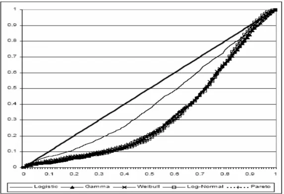
1. Figure 1: Probabilities of Out of Sample 2nd Highest Bids vs U(0,1)………33 2. Figure 2: Probabilities of 3rd Highest Bids vs U(0,1)………37
CHAPTER 1
INTRODUCTION
The aim of this study is to estimate bidders’ private values and an exogenous entry process by maximum likelihood under five different assumptions about the underlying distribution of private values and to estimate the consumer surplus in the market for computer monitors using data from 2934 eBay auctions. The next chapter begins with a review of literature. I then desribe the data set and data collection techniques, present the model and likelihood functions, demonstrate the statistical distributions employed in the analysis and discuss the estimates of the model parameters. Chapter 3 forms the core of this study where I present two types of consumer surplus estimates, the ex-post and the lower bound consumer surplus and a more portable statistic, the consumer share. In chapter 4, I focus on finding the best parametric distribution for private values and employ two different approaches for this purpose. The first approach uses tests based on several well known information criteria to assess model fit. The second one is based on three types of tests against the empirical distribution of private values. The last chapter, chapter 5, concludes by briefly summarizing this study and its implications.
The data set used in this study was retrieved from eBay computer monitor auctions. It is well known that eBay is a significant economic marketplace. It enables trade on a local, national and international basis. Founded in September
1995, eBay is an online marketplace for the sale of goods and services by a diverse community of individuals and small businesses. Presently, the eBay community includes more than a hundred million registered members from around the world, making it the most popular shopping destination on the Internet.1 First introduced in 1995, eBay has proved to be a popular exchange mechanism. According to eBay archives, net revenues totaled $4.552 billion in 2005, which represents an increase of 39% from the $3.271 billion reported in the full year 2004. In 2004, gross merchandise volume of eBay, measured by the total value of all successfully closed listings on eBay’s trading platforms, was $44.3 billion, representing a 30% year over year increase from the $34.2 billion reported in the full year 20042 . The price discovery power of auctions has long been accepted by economists, but the cost of getting bidders together prevented their widespread usage. eBay provided a solution to this problem by creating the environment for people to auction items over the internet. Due to this reason, eBay has become a significant marketplace. It is likely to remain so in the future as evidenced by the economies of the marketplace. Yet, it is not well known how eBay benefits the economy. One measure of this benefit is the consumer surplus eBay generates. This study measures this important attribute in the market for computer monitors.
I estimate bidders’ values and an exogenous entry process using maximum likelihood. Each bidder’s valuation is an independent draw from an absolutely continuous distribution. Since it is not possible to be certain of the true underlying distribution of bidders’ values, I estimate the maximum likelihood function using multiple distributional assumptions. In this way, I am able to estimate consumer surplus under different distributional assumptions and test for sensitivity to
1
http://pages.ebay.com/aboutebay/thecompany/companyoverview.html
distribution. In addition, it allows me to test which distribution best fits the. The data set I use for this purpose consists of 2934 PC color computer monitors with a screen size of between 14 and 21 inches that were auctioned between February 23, 2000 and June 11, 2000. Hasker, et al. (2005) explain in detail the data collection and selection process. The data set was refined by excluding monitors that were not in working order, that were touch screen, LCD, Apple or Macintosh monitors since they were not in the same market. In addition, if bid retractions or cancellations were observed (which happened in 7.4 percent of the auctions), that auction was dropped from the data set on the grounds that bid retractions might indicate collusive behavior among bidders.
eBay has two different auction formats. One is the “Dutch” auction which enables the auctioneer to sell two or more items in the same auction. In this format, bidders specify the number of items they want to buy and their willingness to pay for them. The selling price of the good is equal to the second highest bid (highest losing bid). Since I deal with single-item auctions, I ignore these observations. Second is the common auction format encountered in eBay, English auction with a hard stop time. This is the type of auction used in 87 percent of the data set and the type of auctions on which I focus. At the time the data set was collected, bidding went on from three to ten days and stopped at a preset time. This preset ending time is known as the hard stop time and starts at the second the auctioneer lists the item for sale and ends at exactly three, five, seven or ten days after its start, depending on the auctioneer’s duration choice.
CHAPTER 2
LITERATURE REVIEW, DATA SET, THE MODEL AND
ESTIMATES OF MODEL PARAMETERS
2.1 Literature Review
In the literature, there not many studies which focus on the estimation of consumer surplus though it is an important measure of the benefit users derive from the marketplace. Song (2004) estimates a non-parametric model using both the second and third highest bids in university yearbook auctions. She constructs a new methodology using the second and third highest bids and estimates the median consumer surplus in university yearbook auctions at $25.54. In her research, the median price was around $22.50. This in turn implies that the median consumers’ share of the surplus is 53%. In comparison, I search over parametric models using maximum likelihood. This methodology dispenses with the need to use the third highest bid (which is of questionable trustworthiness) and suggests a best parametric model which might be applicable in other research. In another paper that measures consumer surplus in online auctions, Bapna, et al. (2005) use a new data collection technique that allows them to directly observe a bidder’s stated value. By designing a sniping agent that places last second bids on bidders’ behalf, they collect a large data set consisting of 5157 auctions. Unfortunately, this data set is very heterogenous and they can not estimate a structural bidding function. They compute the median
consumer surplus in all categories at $3.53. The median sales price in their data set is $13.16 which in turn implies that consumers capture at least 21% of the total available surplus in the marketplace. Several other articles have touched on this subject. Carare (2001), Bapna, et al. (2003a), Bapna, et al. (2003b), Bapna, et al. (2004) estimate consumer surplus in multi-unit auctions. However, these papers primarily focus on mechanism design issues and must use ad hoc techniques since the equilibrium bidding function in general multi-unit auctions is unknown. Thus these papers are outside the scope of this study.
The estimation techniques used in this study are based on methods developed by Donald and Paarsch (1993). Unlike that paper, in this study, it is not necessary to estimate the minimum or maximum value a bid can take since in the auctions I consider, the natural lower boundary is zero and there is no reasonable binding upper boundary. I assume it is infinity, with extremely low probability. The data set I use also allows me to estimate a full likelihood function instead of a truncated one, since it includes all auctions where no one decided to bid.
There are several other methodologies currently available in the literature. First of all is the non-parametric technique found by Song (2004). This requires the use of data from the second and third highest bids to provide a non-parametric estimate of bidders’ value distribution. For clear theoretic reasons, one can always assume that the second highest bid is a bidder’s true value; the bidder decreases her probability of winning the auction by shading her bid and bidding her true value does not affect the price she will pay if she wins since the item is sold at the second highest bid. However, the same guarantee does not exist for the third highest bids since one has to rely on the bidders’ not planning to update their bids, which they frequently do. This type of bidder behaviour could potentially bias the results. In
addition, non-parametric techniques have the problem of slow convergence. Furthermore, while my parametric models are more restrictive, finding the best fit is more informative than with non-parametric techniques. With non-parametric techniques, comparing distributions for different goods is diffcult, with parametric maximum likelihood, I can easily compare my results across different product categories and observe if there is some fundamental underlying distribution of values.
Another technique encountered in the literature is a Bayesian methodology developed in Bajari and Hortaçsu (2003). These techniques require that the bidding functions be linearly scalable, a restriction unnecessary with this study’s approach and violated by the structural form. A final technique is a Non-Linear Simulated Least Squares methodology developed by Laffont, et al. (1995). This approach overcomes the complexity of calculating the likelihood function by simulating the auctions, and is a flexible methodology that can be used for many models where revenue equivalence holds. Hasker, et al. (2005) employs this technique. In this study, I choose to use maximum likelihood estimation, since it is feasible and is the more standard approach.
2.2 Data Set and Collection Techniques
∗∗∗∗At the time the data set I use in this study was collected, eBay saved all information about closed auctions on their website for a month after the auction closed. This allows people who participated in the auction to verify the outcome, and provides the source of my data set. Data was collected using a “spider” program which periodically searches eBay for recently closed computer monitor auctions and
downloads the pages giving the item description and the bid history. Software development was done in Python-a multi-platform, multi-OS, object–oriented programming language. It is divided into three parts. It first goes to eBay’s site and collects the item description page and the bidding history page. It next parses the web, and makes a database entry for each closed auction. The final part iterates through the database entries stored, and creates a tab-delimited ASCII file.
The original data processing program did not process all of the data. It provided the researcher with the core of the data which was augmented with further processing of the raw html files. Using string searches, extensive descriptive information for the entire data set was collected. Further data processing enabled one to collect all of the bidding histories.
This program was run from February 23, 2000 to June 11, 2000 collecting information on approximately 9000 English auctions of computer monitors, which, in effect, constitute all monitors auctioned during that time period. To arrive at the final data set, Hasker, et al. (2005) had to drop many of these monitors because they are not in the same market as PC color computer monitors with a size between 14 and 21 inches. They dropped all monitors that were not in working order, were touch screen monitors, LCD monitors, Apple monitors and other types of monitors that are bought for different purposes than the monitors in the final sample. In addition, if there were any bid retractions or cancellations, which was the case in 7.4% of the auctions, they dropped the data point. This was done because bid retractions might indicate collusion among bidders. Cancellations happened in a few auctions where the auctioneer cancelled the auction early (usually within ten to fifteen minutes of the beginning of the auction) causing that auction to be dropped. For the purposes of this study, it was necessary to further drop some of the observations in order to construct
measures of the competition each auction faced, resulting in 2934 auctions to be used in my estimations. The amount of competition a given auction faces is best reflected by the number of auctions which were open while it was open. Hence, it was necessary to drop auctions that were within ten days of a break in the data collection. I then counted the number of auctions, including the given auction, that were open, open and had the same size of monitor, or open and were in the same category. This resulted in three variables that measure the amount of competition an auction faces.
Descriptive variables except for monitor size were constructed using string searches. Hasker, et al. (2005) detailly explain the strings that were used for each variable. This allowed one to collect data on whether there was a secret reservation price, whether it was met, monitor resolutions, dot pitch, whether a warranty was offered, several different brand names, whether the monitor was new, like-new, refurbished (the omitted category is Used), and whether it was a flat screened monitor. “Brand name” is used for monitors that are from one of the ten largest firms represented in the data set. These firms are Sony, Compaq, NEC, IBM, Hewlett Packard, Dell, Gateway, Viewsonic, Sun, and Hitachi in order of size. Sony has around a 10% market share, the smallest are all around 3%, in total these 10 firms represent 57% of the market. Dot pitch (DPI) and resolution are not reported in all of the auctions. DPI is reported in 35% of the auctions, resolution in 58%. In the appendix the descriptive statistics of variables of interest are presented.
2.3 The Model and Likelihood Functions
I will use maximum likelihood technique to estimate bidders’ values and an exogenous entry process in eBay auctions. Prior to defining the model and estimation method in more detail, let me briefly explain the proxy bidding mechanism used in
eBay. Every bidder willing to participate in a given auction submits a maximum bid showing his current willingness to pay for the auctioned object. This bid is subject to change and does not necessarily reflect the true value of the bidder. The bidder can increase his bid if he wishes but cannot decrease it. The proxy bidding program then issues a proxy bid which is equal to the second highest bid plus one bid increment. This amount is displayed next to a current winner’s identity. This process continues until only one bidder is left in the auction. When the auction terminates, the winner is awarded the item at a price equal to the second highest bid plus one bid increment. There are two exceptions to this rule. In the special case where the actual number of bidders is one, sales price equals the open reservation price (in auctions without a secret reserve). The other special case occurs when the two highest bidders submit the same amount. In such a situation, winner is determined based on bid submisson time, the earlier bidder winning the auction. If ties occur, winner is determined by a completely randomized process. The winner pays an amount equal to his actual bid.
In eBay English auctions the obvious action is to enter one’s true value (or simply “value”) as his bid. However, frequently bidders do not do this, so to be certain that at least the second highest bidder does, I will follow Haile and Tamer (2003) by assuming that bidders’ bidding strategy satisfies the following two rules: 1. No bidder ever bids more than he is willing to pay.
2. No bidder allows opponents to win at a price he is willing to pay.
Haile and Tamer (2003) show that these two assumptions imply that if ( I2: )
b is the second highest bid among I potential bidders, then w (2:I) (2:I)
v b b = = , where w b and ) : 2 ( I
b denote the winning bid (sales price) and the second highest bid among I
potential bidders, respectively.
of auction specific characteristics xn(where n indicates the auction) and a private
component ρj (where j indicates the person). To be more explicit, bidder i’s private
value in auction n is given by the equation: i n x i n n
e
v
=
'βρ
(1) If w nb is the winning price, rn is the traditional open reservation price, i n
ρ is the private component of the ith potential bidder in the nth auction and I is the potential number of bidders who considered bidding in the auction, the formula for the winning bid is:
{
ln , ' ln (2:)}
max ln I n n n w n r x b = β + ρ (2) where ( I2:) nρ is the private component of the second highest bidder in auction n. In other words, sales price is equal to either the open reservation price or the value of the second highest bidder, whichever is greater. I will allow for various models of the distribution of values, i
n
v , and thus the distribution of bnw .
Let Fn(z;β) be the cumulative distribution function (cdf) of bidders’ private values at z and fn(z;β)be the probability density function (pdf) – where β may include some distribution specific coefficients. Let a
n
I be the number of active bidders in auction n, or the number who actually submitted bids, and for i∈
{ }
0,11 = i n D if Ina =i, i =0 n
D otherwise. If I ≥Ina is the number of potential bidders in auction n, then the likelihood of auction n given I is :
)
|
(
I
l
nβ
=
(
(
;
)
I)
Dn0*
n nr
F
β
(
(
1
(
;
))
(
;
)
I 1)
D1n*
n n n nr
F
r
F
I
−
β
β
−(
)
1 0 1 2(
1
(
;
))
(
;
)
)
;
(
)
1
(
w Dn Dn n n w n n I w n nb
F
b
f
b
F
I
I
−
β
−−
β
β
− − (3)In any given time, it is not possible to measure how many inactive bidders there might be. It is certain that there have been at least a
n
I bidders who have thought about bidding (and bid), but there may have been any number of bidders who thought about bidding but did not. For this reason, I will be a stochastic variable that can range from a
n
I to
−
I - an arbitrary upper bound.
The potential number of bidders in an auction will be determined by a Poisson entry process. The parameter of the entry process, λn, will be log-linear in a
set of auction specific characteristics, zn, where xn ⊆ zn. Some auction
characteristics might affect entry but not bidders’ values, but I assume that if the auction characteristic affects values, it must affect entry. The estimared functional form for entry is:
lnλn =zn'γ (4) Let Tn be the length of the auction in days (Tn∈
{
3,5,7,10}
) andsr n
D be a dummy which is one if there is a secret reservation price. Then the total likelihood function for auction n is:
∑
∑
− − = − + = −=
I D i T i n n I D I i n T i n n n sr n n n sr n a n n ne
i
T
i
l
e
i
T
l
λ λλ
β
λ
γ
β
!
)
(
)
|
(
!
)
(
)
,
(
(5) a nI is increased by one if there is a secret reservation price, thus I am following Bajari and Hortaçsu (2003) in treating the auctioneer as another bidder if there is a secret reservation price.
general, data only includes auctions that result in a sale, making this study a rare example of full maximum likelihood estimation in auctions.
The choice of −Iis obviously arbitrary. To derive the estimates I chose =30
−
I and then tested the results when =50
−
I . This change did not alter the coefficients, thus it appears the choice of =30
−
I is sufficient.
2.4 The Distributions
It is not possible to be certain a-priori what the true distribution of bidders’ private values is. For this reason, I test several different distributions: the logistic, gamma, weibull, lognormal and pareto.
The pdf of the logistic is:
β β β
β
' ' '1
1
1
1
)
;
(
1 1 n n x n x x e z e z ne
e
e
z
f
+
−
+
=
− − − − (6)Notice that this distribution does not have a distribution specific parameter. The pdf of the gamma is:
( )
β α β αα
β
' ' 1)
(
1
)
;
(
xn n e z x ne
e
z
z
f
− −Γ
=
(7)where I writeβ =
{
β,σ}
for notational simplicity. The parameter α > 0 is the shape parameter of this distribution and I estimate lnα to prevent this parameter from being negative.The pdf of the weibull is:α β α β α
α
β
− −=
' ')
(
)
;
(
1 n x n e z x ne
e
z
z
f
(8)where againβ =
{
β,σ}
. The parameter α > 0 is the shape parameter of the weibull distribution, and αln is estimated. The pdf of the lognormal is:2 2 ' ) /2 (ln
2
1
)
;
(
β σπ
σ
β
z xn ne
z
z
f
=
− − (9)where β =
{
β,σ}
for simplicity of notation. The pdf of the pareto is: ) 1 ( ' '1
)
;
(
+ −
+
=
α β βα
β
n n x x ne
z
e
z
f
(10) where againβ ={
β,σ}
, α is the shape parameter of this distribution and lnα isestimated.
2.5 The Estimates
I first present the estimates of the exogenous values ( β
'
n
x
e
) and then I present my estimates of the parameter of the entry process (lambda). In the model, the right hand side variables for the exogenous values are the size of the monitor (diagonal screen size), the dot pitch (the distance between dots on the screen), resolution (the size of picture that can be seen on the monitor). In addition, there are a series of dummies indicating whether or not the monitor is new, like-new, or refurbished (the omitted category is “used”) and whether or not the monitor has a warranty, is a brand name, or is flat panel.Table 1: Estimates of the Exogenous Value of a Monitor
Logistic Gamma Weibull Lognormal Pareto Constant -11.3159*** (0.000) -11.1785*** (0.000) -13.7639*** (0.000) -14.3522*** (0.001) -12.1096*** (0.006) Log, Size 4.6806*** (0.004) 4.8012 (0.894) 4.7326*** (0.000) 4.806*** (0.000) 4.6192*** (0.000) Log, Dot Pitch -0.5418
(0.793) -0.7289 (0.500) -0.5844 (0.425) -1.1047 (0.563) -0.2101 (0.912) Dummy, No Dot Pitch 0.6132
(0.487) 0.8606 (0.521) 0.6666 (0.815) 1.366* (0.055) 0.1142 (0.872) Log, Resolution 0.1409 (0.911) 0.1695 (0.992) 0.2811 (0.168) 0.1448 (0.717) 0.307 (0.441) Dummy, No Resolution 1.0803 (0.415) 1.309 (0.786) 2.0814** (0.025) 1.0922 (0.107) 2.2261*** (0.001) Dummy, New 0.2539 (0.864) 0.3345 (0.907) 0.3242 (0.945) 0.3939 (0.149) 0.3203 (0.241) Dummy, Like-new 0.0877 (0.960) 0.2247 (0.923) 0.2351 (0.802) 0.3396 (0.188) 0.2425 (0.347) Dummy, Refurbished 0.0594 (0.998) 0.0619 (0.987) 0.0482 (0.998) 0.04 (0.965) 0.0204 (0.982) Dummy, Warranty 0.0779 (0.935) 0.0976 (0.952) 0.1033 (0.959) 0.189 (0.798) 0.1154 (0.876) Dummy, Brand Name 0.016
(0.861) 0.0061 (0.996) 0.0055 (0.997) 0.009 (0.990) -0.001 (0.999) Dummy, Flat Screen 0.1979
(0.733) 0.246 (0.618) 0.2246 (0.645) 0.2213 (0.592) 0.2047 (0.620) Distribution Variable+ NA -1.695 (0.762) -0.6841 (0.527) 1.6563*** (0.000) 0.7099** (0.022) Number of Auctions 2934 2934 2934 2934 2934 -Log Likelihood/Number of Auctions 3.7939 3.7175 3.7583 3.8402 3.8441
Note 1:+ indicates standard deviation estimate for the lognormal distribution. For the weibull,
gamma and pareto distributions, it indicates the log of the shape parameter estimate. Note 2: p-values are reported below the coefficients in parentheses.
Note 3: * , ** and *** indicate significance at the 10%, 5% and 1% levels, respectively
Table 1 reports the results. I first note the general stability of coefficients across estimates. The least stable coefficients are those for dot pitch and resolution, and even in these cases, the ratio of the coefficient on the variable to the dummy for that variable not being reported is fairly stable-generally -0.80 to -0.85 for dot pitch (with the exception of the pareto distribution) and 0.13 for resolution. The coefficient on brand name does change sign in one regression and is never significant, probably because brand name really conveys to the bidder that the monitor is a common brand. The coefficient of the diagonal screen size variable is estimated as approximately
five in all distributions and it is significant except for the gamma case indicating that buyers prefer bigger sized computer monitors.
While the differences in coefficients are generally small, the exogenous value
( )
xn'βe
of a computer monitor can be very different for a given auction using the different techniques. In Table 2 I report the descriptive statistics of the logs of predicted exogenous values since the exponential function creates a skewed distribution and significantly biases the mean.Table 2: Log of Predicted Exogenous Values (xn'β)
Logistic Gamma Weibull Lognormal Pareto Average 3.63 4.58 2.38 1.74 3.33 Exponential of Average $37.71 $97.51 $10.80 $5.70 $27.94 Median 3.64 4.57 2.37 1.72 3.32 Exponential of Median $38.09 $96.54 $10.70 $5.58 $27.66 Standard Deviation 0.71 0.74 0.73 0.75 0.72 Minimum 2.56 3.45 1.21 0.63 2.18 Maximum 5.32 6.47 4.26 3.83 5.18
The exponential of the average and median are in dollar terms, thus I discuss these variables. As the results indicate, these two estimates are almost the same for a given distribution but they vary widely across distributions showing that a monitor’s exogenous value is very sensitive to the underlying distribution of bidders’ private values. The gamma distribution produces the highest estimate ($98), followed by the pareto and the logistic which produce medium values ($28 and $38 respectively) and the lognormal and weibull distributions produce very low values ( $6 and $11 respectively)
Next, I present the estimates of the entry process. To estimate the entry variable lambda, I use all variables that affect bidders’ values and other variables that only affect entry. The first two additional variables are the log of the seller’s feedback and
experience. In eBay, the winner and the seller can rate each other as negative, neutral or positive which correspond to -1, 0, 1 feedback points, respectively. A seller’s feedback rating is the sum of all these feedback points. Thus, feedback increases by one with every sale that results in a pleased customer and this variable is a measure for both the seller’s reputation and experience. There are also a series of category dummies. The default is the “general” classification but a seller is allowed to put the monitor into the ≤ 17″ screen, ≥19″ screen or the monotonic subcategories if he
wishes. All monitors that are put in the monotonic sub-category are misplaced since all monitors in the data set I use are color monitors. In addition, there are three variables that capture the amount of competition a given auction faces. The variables, (competing auctions, all), (competing auctions, same size) and (competing auctions, same category) are created for this purpose. The data collection process captured every monitor auctioned during the sampling period which in turn enabled me to construct these competition variables. The first of these variables, (competing auctions, all), is simply the number of other auctions that were open while the auction was running, divided by the length of the auction. The second variable (competing auctions, same size), shows how many of those open auctions had a monitor of the same size, normalized again, by the length of the auction. The final variable (competing auctions, same category) is the number of open auctions in the same category, normalized also by the length of the auction. Table 3 reports the estimates.
An examination of the estimates reveal that they are less stable than the estimates of bidders’ exogenous values. However, the signs of the coefficients are generally stable, only in six out of twenty two variables, do I observe a sign change. The signs of the coefficients are, in general, consistent with my expectations. On the
other hand, the coefficient of the secret reservation price dummy is positive in all models, contrary to my expectations, but it is extremely insignificant in all specifications. Theoretically, the presence of a secret reservation price deters bidders from entering an auction contrary to what my estimation process yields. Thinking that this variable may be correlated with the error term, I tried instrumenting this variable on all the rest and the subsets of the remainig variables and also, allowed for a different probability for the first bidder to arrive. Neither of these techniques have changed the estimates. I think the most likely reason is that secret reservation prices are used on items with an extremely high value. Thus entry to these auctions will be more and the log-linear model of entry can not capture this. In effect, even if I control for the effect of the secret reservation price on entry, auctions with a secret reservation price generally can expect 50% more bidders than auctions without a secret reservation price.
The coefficient on the open reservation price variable has a negative sign except for the lognormal distribution specification, where it has the wrong sign. It is well known that on eBay, auctioneers are not willing to raise the open reservation price in order not to scare bidders away. However, in all cases, this coefficient is highly insignificant, indicating that bidder behavior is essentially unaffected by the announced reservation price.
The coefficients on the competition variables yield interesting results. The coefficient on the competing auctions-all variable is consistently positive and significant in all distribution specifications. This implies that increasing the number of competing auctions increases the likelihood that a bidder will enter a given auction.
Table 3 : Estimates of the Entry Process
Logistic Gamma Weibull Lognormal Pareto Constant -15.5587*** (0.000) -13.033*** (0.000) -14.5406*** (0.000) -5.1905*** (0.000) -16.1312*** (0.000) Log, Size 3.3723*** (0.000) 3.2725*** (0.000) 3.4683 (0.463) 4.2382*** (0.000) 3.8408*** (0.000) Log, Dot Pitch -5.4067
(0.637) -7.2483* (0.080) -8.4491*** (0.006) -3.4813 (0.992) -7.9655 (0.981) Dummy, No Dot Pitch 6.5705***
(0.000) 8.5044*** (0.000) 10.0708*** (0.000) -3.3655*** (0.000) 9.6205*** (0.000) Log, Resolution -0.8514 (0.968) -1.4036* (0.097) -1.5012*** (0.000) -1.2527 (0.316) -1.3859 (0.267) Dummy, No Resolution -6.0989*** (0.000) -10.0171*** (0.000) -10.7186 (0.130) -8.966 (0.554) -9.8957 (0.514) Dummy, New 7.3845 (0.983) 7.4000 (0.999) 7.5104 (0.998) 5.5506 (0.990) 7.5072 (0.987) Dummy, Like-new 6.5463 (0.979) 6.5000 (1.000) 6.0767 (0.996) 3.0008 (0.916) 6.0748 (0.831) Dummy, Refurbished -0.0011 (1.000) -0.0205 (0.991) 0.0039 (0.999) 0.0161 (0.986) 0.0366 (0.968) Dummy, Warranty 0.4447 (0.573) 0.8402 (0.964) 0.971 (0.741) 0.7463 (0.488) 1.0831 (0.315) Dummy, Brand Name -0.0075
(0.998) 0.0128 (0.999) 0.0092 (0.989) -0.006 (0.966) 0.0147 (0.917) Dummy, Flat Screen -0.0549
(0.967) -0.2003 (0.964) -0.183 (0.797) -0.1187 (0.974) -0.2295 (0.951) Log, Seller's Feedback +1 0.715
(0.992) 1.5201*** (0.002) 1.4805*** (0.000) 2.2702*** (0.000) 1.7373*** (0.004) Log, (Seller's Feed Back+1)2+1 -0.3473
(0.955) -0.7443*** (0.006) -0.7198*** (0.002) -1.1072** (0.021) -0.8432* (0.079) Category Dummy, 17 Screen 0.8153*
(0.094) 1.1007*** (0.001) 0.9541 (0.114) 0.8032 (0.205) 0.7102 (0.262) Category Dummy, 19 Screen 0.1085
(0.951) 0.2498 (0.717) 0.1388 (0.897) -0.2512 (0.931) -0.0794 (0.978) Category Dummy, Monotonic -1.5328***
(0.002) -1.6876 (0.283) -1.411 (0.989) -0.7847 (0.227) -1.1656* (0.073) Competing Auctions, All 1.2191***
(0.007) 1.1813** (0.014) 1.1274** (0.014) 1.0966** (0.021) 1.0732** (0.024) Competing Auctions, Same Size 0.2364
(0.738) 0.241 (0.629) 0.2373 (0.914) 0.1552 (0.797) 0.2319 (0.701) Competing Auctions, Same Category -0.2957
(0.886) -0.3409 (0.341) -0.2529 (0.317) -0.0674 (0.877) -0.1192 (0.785) Open Reservation Price -0.0754
(0.997) -0.0253 (0.983) -0.0199 (0.980) 0.005 (0.994) -0.0206 (0.976) Dummy, Secret Reserve 0.5861
(0.916) 2.2273 (0.952) 1.1178 (0.152) 1.3458 (0.916) 1.0856 (0.932) Number of Auctions 2934 2934 2934 2934 2934 -Log Likelihood/Number of Auctions 3.7939 3.7175 3.7583 3.8402 3.8441
Note 1:+ indicates standard deviation estimate for the lognormal distribution. For the weibull,
gamma and pareto distributions, it indicates the log of the shape parameter estimate. Note 2: p-values are reported below the coefficients in parentheses.
Note 3: * , ** and *** indicate significance at the 10%, 5% and 1% levels, respectively
eBay’s market power stems from economies of marketplace, and this coefficient dramatically illustrates this point. The main reason why buyers prefer eBay over its competitors is that there are many sellers in eBay. Similarly, sellers prefer to auction
items using eBay because there are many buyers using eBay. Thus, I cannot be certain that increasing the number of auctions will decrease the number of bidders per auction and competition coefficients support this insight. Note that increasing the number of competing auctions in an item’s category decreases the number of bidders per auction. These effects may vanish in a current data set where the number of bidders per auction are much greater than they were in this study’s data’s collection period. It is interesting to be able to find empirical support of the theoretic reason for eBay’s success.
The dummy variable, no dot pitch, shows whether the auctioneer chose to report the dot pitch in his auction or not. The coefficient on this variable is positive except for the lognormal specification. For the rest of the four specifications, not reporting dot pitch increases entry for a given auction. However, in the lognormal specification, I see that not reporting dot pitch deters entry. Except for the lognormal case, the ratio of the coefficient on the dot pitch variable to that on the dummy variable for not reporting dot pitch is stable and takes values around -0.85. Similarly, the ratio of the coefficient on the resolution variable to that on the dummy variable for not reporting resolution is stable in all five cases, and takes a value around 0.14. In Table 1 one sees that increasing an item’s resolution increases its value to bidders. However, it seems to adversely affect the entry process, and lower the expected number of bidders. This indicates that some heterogeneity exists among bidders. A high resolution means that, for a given screen size, it is possible to see a larger picture or page of text. This also means that the details of the picture or the text size are smaller, and it is reasonable to conclude that some bidders do not want to pay more for such a monitor. My results indicate that some bidders do not value resolution and thus are not willing to bid on items with a high resolution. By looking
at the coefficient estimates on the dummy variable for flat screen monitors in tables 1 and 3, I see that the same tendency exists (though to a lesser degree) in flat screen monitors; although a flat screen increases a monitor’s value, due to the heterogeneity in bidders’ preferences, entry is adversely affected by flat screen monitors. While a flat screen is a positive aspect, not everyone will be willing to pay more for it, and this has a small negative effect on entry and a small positive impact on the item’s value. Analysis of the coefficients on the variables, refurbished and brand name, yield somewhat similar results, though this result is dependent on distribution specification. A monitor’s being refurbished slightly improves its value in all five specifications, but its impact on entry is specification dependent. Likewise, a monitor’s being a brand name monitor slightly increases its value in all five specifications, except for the pareto case. Its impact on bidder entry process is, again, specification dependent.
Analysis of the coefficients on the two seller’s feedback-related variables displayed in Table 3 helps one assess the impact of the seller’s reputation and experience on the potential number of bidders. The coefficient on the log of seller’s feedback is significant and positive in all specifications except the logistic. The coefficient on the log of seller’s feedback square captures the marginal impact of increasing feedback rating on the entry process. This coefficient is consistently negative in all specifications, indicating a diminishing marginal impact of increasing feedback. These coefficients deserve special attention, since there are two reasons that we should expect a significant and positive impact for feedback. First reason is that more experienced auctioneers know more about setting up auctions; they use clearer item descriptions, use pictures, etcetera. These things encourage bidders to enter the auction. Second is that these coefficients in a way reflect bidders not
trusting a seller who has a lot of negative feedback. Indeed, Cabral and Hortaçsu (2004) follow auctioneers over time and find that one negative feedback can decrease the growth rate of an auctioneer’s sales from 7% to -7%.
While the estimated model of entry varies dramatically across regressions, the expected number of bidders varies less than the exogenous values do. Again, I report the descriptive statistics of the log of the entry parameter lambda, since the exponential function introduces a significant right skewness to the distribution. Table 4 displays the results.
Table 4: Predicted Values for the Log of Entry Parameter
Logistic Gamma Weibull Lognormal Pareto Average 2.01 2.86 2.63 5.04 2.49 Exponential of Ave. 7.5 17.46 13.9 154.5 12.1 Median 1.28 1.93 1.82 2.32 1.7 Exponential of Med. 3.6 6.89 6.2 10.2 5.5 Standard Deviation 2.33 2.66 2.51 4.52 2.48 Minimum -0.94 -0.92 -1.03 -1.07 -1.29 Maximum 11.46 13.74 12.87 18.00 12.70
Comparing the average and the median values, one sees that they are significantly different from each other, indicating to a right skewness in the distribution of lambda. Hence, it is more reliable to interpret the median. For the gamma, weibull and pareto distributions, the estimates of lambda are essentially the same. The median number of bidders per day is around 6-7. However, the logistic and lognormal results deviate from this pattern. Logistic reveals a low estimate, 3-4 bidders per day, whereas the lognormal yields a high estimate, around 10 bidders per day. Since I use a Poisson entry process to model entry, lambda is equal to the expected number of bidders per time period, per one day based on my data set. Thus, in a three day auction, the median number of bidders is estimated to vary between 10 and 30, in a ten day auction, between 35 and 100. Even the most conservative
estimates suggest that there is a large number of potential bidders for each computer monitor, once again providing empirical evidence for the popularity of eBay auction market.
CHAPTER 3
CONSUMER SURPLUS AND CONSUMER SHARE
3.1 Consumer Surplus
Today internet auctions provide a popular means of transaction for numerous buyers and sellers. One important issue about internet auctions is the amount of consumer surplus that buyers derive from them. If this amount is low bidders can easily switch to other methods of transaction given the competing markets. In this section, I attempt to measure this consumer surplus given the various distributional specifications.
The ex-post consumer surplus is the difference between the winner’s value of the item being auctioned and what she actually paid for it. While the a-priori consumer surplus, the surplus a bidder expects before entering the aution, is a function of the potential number of bidders, I, the ex-post consumer surplus is not and therefore estimating ex-post consumer surplus is relatively straightforward. This is in part because I do not have to calculate a summation over the possible values of the potential number of bidders.
One point is important and needs to be clarified at this stage. After an auction closes, eBay lists the complete bid history with the exception being the actual amount submitted by the winning bidder. This information is never disclosed, neither during nor after the auction. Since I can not observe the highest bidder’s valuation in
the conditional expectation of the highest bidder’s valuation given the second highest bid. Due to the theoretical reasons pointed out in section 3, I fail to reject that the winning bid (sales price) is the second highest bidder’s value of the goood. (I assume that the bid increment in eBay is zero). From this discussion it follows that the ex-post consumer surplus in auction n is :
(
)
nw w n I n I n v b I b v E (1: ) | (2: ) = | ≥1 − (11) if I let w n w n b r = when I = 1, where w nr denotes the open reservation price. This is because, if there is only one bidder in the auction and the item is sold, it is sold at the reservation price. For all I ≥1 the expression above is the same as :
w nw n n b n
b
b
F
dz
z
zf
w n−
−
∫
∞)
,
(
1
)
,
(
β
β
(12) The proof is done by simplifying(
)
wn w n I n I n v b I b v E (1:) | (2:) = | ≥2 − to show that it is equal to
(
)
w n w n I n I n v b I b vE (1:) | (2:) = | =1 − , which is the above expression.
Lemma 1 If I ≥1 then ex-post consumer surplus is independent of I, and thus independent of the entry process.
Proof. The explicit form of the expectation is :
(
)
2 2 ) : 2 ( ) : 1 ())
,
(
)(
,
(
))
,
(
1
)(
1
(
))
,
(
)(
,
(
)
,
(
)
1
(
2
|
|
− ∞ −−
−
−
=
≥
=
∫
w I n n w n n w n n b I w n n w n n n w n I n I nb
F
b
f
b
F
I
I
dz
b
F
b
f
z
zf
I
I
I
b
v
v
E
w nβ
β
β
β
β
β
=
1
(
,
)
)
,
(
β
β
w n n b nb
F
dz
z
zf
w n−
∫
∞=
E
(
v
n(1:I)|
v
n(2:I)=
r
n|
I
=
1
)
if I let n w n r b = when I = 1.statistics for estimates of consumer surplus for the various distributions I consider are reported in Table 5.
Table 5: Expected Consumer Surplus
Logistic Gamma Weibull Lognormal Pareto Average $90.29 $89.40 $106.64 $194.81 $160.08
Median $38.68 $68.32 $82.69 $142.95 $114.08 Standard Deviation $1,582.60 $72.35 $89.01 $177.66 $151.32 Minimum $13.51 $7.94 $7.38 $7.66 $9.61 Maximum $68,068.00 $473.21 $544.27 $1,461.20 $1,472.90
It is evident from these estimates that expected consumer surplus is affected by the underlying distribution of bidders’ private values. There is a wide variation in these estimates across distrinutions. In my data set, median selling price for a computer monitor is $100. Thus, these estimates are high. Comparing average and median consumer surplus values, one sees that average is always greater than the median, indicating a significant right skewness. For this reason, using the median estimates for interpretation is more reliable. The logistic produces the lowest estimate, whereas the lognormal yields the highest. The gamma produces the next lowest estimate after the logistic. Notice that their averages are nearly the same. Pareto, following the lognormal, produces the second highest estimate. It is important to note that these two distributions are the worst fitting ones.
3.2 Consumer Share
An alternative and more portable way of presenting these statistics, instead of finding the absolute consumer surplus, is reporting the consumer’s share of the surplus. If vb is the buyer’s value and va the auctioneer’s value, then this statistic is
w n
b b
v −
not possible to accurately estimate va from the data. For this reason, I assume that,
0 =
a
v which gives me a lower bound. These estimates are reported in Table 6.
Table 6: Expected Consumer Surplus Share
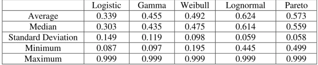
Logistic Gamma Weibull Lognormal Pareto Average 0.339 0.455 0.492 0.624 0.573
Median 0.303 0.435 0.475 0.614 0.559 Standard Deviation 0.149 0.119 0.098 0.059 0.058 Minimum 0.087 0.097 0.195 0.445 0.499 Maximum 0.999 0.999 0.999 0.999 0.999
Expected consumer share estimates gives one information about how much of the total available consumer surplus bidders are capturing. Despite the fact that there are many bidders per computer monitor auction, consumers are still receiving between one third and two thirds of the generated surplus.
3.3 Lower Bound Estimates
Considering the high expected consumer surplus estimates and their wide variation among distributions, I decided to construct a “lower bound” for the true consumer surplus. This statistic will enable me to check the sensitivity of my estimates to the tails of my distributions since it is independent of the distributional assumptions. If the actual number of bidders, I, was constant among auctions, then assuming that w n I n I n v b
v(1:) = (2:) = in every auction would provide me with a strict lower bound on the distribution of private values. Since I is random in my auctions, this estimate does not give me a true lower bound. However, it is still useful in the sense that it enables me to reconstruct my estimates using its empirical distribution and produces estimates that are independent of the tails of the distribution. Table 7 displays the estimates.
Table 7: Lower Bound Estimates of Consumer Surplus
Logistic Gamma Weibull Lognormal Pareto Average $61.29 $61.50 $61.75 $61.28 $61.68 Median $41.38 $40.88 $41.02 $40.08 $41.64 Standard Deviation $53.10 $54.92 $53.55 $53.19 $53.22 Minimum $0.00 $0.00 $0.00 $0.00 $0.00 Maximum $1,022.30 $1,043.00 $931.86 $730.20 $925.59
These lower bound estimates of consumer surplus are more stable across distributions than those in Table 5 and are also comparable given the median sales price of $100. In addition, these estimates are not correlated with the exogenous value of a computer monitor, β
'
n
x
e
. In a similar fashion, lower bound estimates for consumer’s share of surplus are computed and are reported in Table 8.Table 8: Lower Bound Estimates for Consumer Share
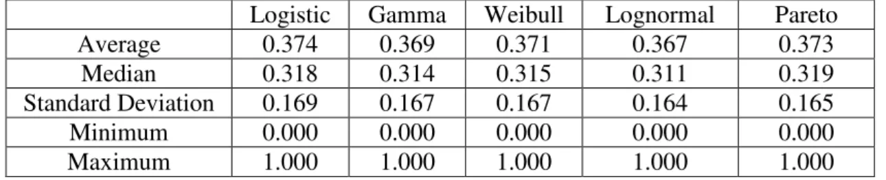
Logistic Gamma Weibull Lognormal Pareto Average 0.374 0.369 0.371 0.367 0.373 Median 0.318 0.314 0.315 0.311 0.319 Standard Deviation 0.169 0.167 0.167 0.164 0.165 Minimum 0.000 0.000 0.000 0.000 0.000 Maximum 1.000 1.000 1.000 1.000 1.000
These estimates yield that consumers capture approximately 32% of the surplus generated in an auction. Accepting that lower bound estimates yield the worst case, consumers are still capturing nearly 32% of the surplus in an auction. Therefore, both the expected and the lower bound estimates reveal that consumers capture a significant portion of the consumer surplus.
CHAPTER 4
FINDING THE BEST DISTRIBUTION
I made five different, parametric distributional assumptions for the underlying distribution of bidders’ private values. It is essential to detect which one best fits the data. For this purpose, I will employ two different approaches. Firstly, I will carry out tests based on the log-likelihood. Akaike (1973) proposes selecting the model that minimizes an information criterion based on the likelihood. Other analysts have suggested other information criteria since that time, and I will compare several of them. In addition, McFadden (1974) provides an analog to the 2
R in a conventional
regression, the likelihood ratio index (LRI), sometimes also called the pseudo 2
R , given by, 0 ln ln 1 L L LRI = −
where lnL is the log-likelihood function with all the model parameters from the model and ln L is the log-likelihood function only including a constant term. As 0 with the measure of 2
R , this index is bounded between 0 and 1. If all the slope
coefficients are zero, then it equals zero, indicating that none of the explanatory variables is indeed useful.3 The LRI increases as the fit of the model improves.
Secondly, I will do tests against the empirical distribution of the second and third highest values. For this purpose, I will take a subset of my data that is not used in estimation and see whether the distirbution of this subset is close to the empirical distribution. I do this by finding the probability of each observation and the distribution of these probabilities should be uniform by construction. I have two different data sets that I can use for this approach. First I did not use half of my data so that I could have variables stating the amount of competition each auction faced. Notice that the data collection program sampled the entire population of monitors in eBay’s records, but in order to know how much competition an auction faces I must know how many auctions closed during a given auction. This led me to drop a significant subset of my data, a subset which I can use now. I can also use a technique that Song (2004) used in her estimation methodology. While one can not trust all third highest bids to reflect the true value of the third highest bidder, one can trust a subset of them, and I can use this subset to test whether my assumed distribution is close to the empirical distribution.
4.1 Tests Based on the Log Likelihood
Since I have multiple distributional assumptions it is important that I find the best fitting one for my data set. To this end, I will employ several information criteria, which are all very similar given my models. These criteria were intended to compare models which are very different in the number of parameters or observed variables. These numbers are nearly constant across my different models. Hence, the tests simplify to checking which distributional assumption yields the largest likelihood value, or similarly, which one yields the smallest negative log-likelihood
The first information criterion I employ is the Akaike Information Criterion: k N L N AIC =− 1 log ( , )+ 1 ∧ ∧ γ β (13)
where N is the sample size, L(β∧,γ∧) is the log-likelihood, and k is the number of parameters. Another criterion that puts more of a penalty on complexity is the Bayesian Information Criterion or the Schwartz Criterion:
k N N L N BIC 2 ) log( ) , ( log 1 + − = ∧ ∧ γ β (14) The final information criterion is the Browne-Cudeck Criterion which is given by the equation: k p N L N BCC 2 1 ) , ( log 1 − − + − = ∧ ∧ γ β (15)
where p is the number of observed variables. Given that N = 2934, p = 21 and
{
34,35}
∈
k , the difference in these statistics is small.
Table 9: Results of the Tests Based on Likelihood
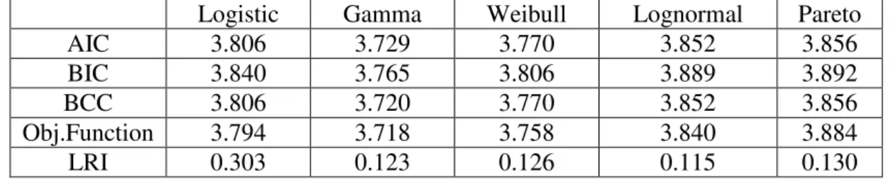
Logistic Gamma Weibull Lognormal Pareto AIC 3.806 3.729 3.770 3.852 3.856 BIC 3.840 3.765 3.806 3.889 3.892 BCC 3.806 3.720 3.770 3.852 3.856 Obj.Function 3.794 3.718 3.758 3.840 3.884 LRI 0.303 0.123 0.126 0.115 0.130
According to AIC, BIC, BCC and objective function values, the gamma specification provides the best fit. It is followed by the weibull, logistic, lognormal and pareto distributions. However, the statistics do not vary widely among distributions. The gamma specification provides a slight improvement over other specifications, 1.1% over the weibull, 2% over the logistic, 3.2% over the lognormal and 4.3% over the pareto. These percentage improvements are subject to change if the same
calculations are to be done with the likelihood values instead of the log-likelihood. On the other hand, LRI values yield a different result. The logistic specification, which has the highest pseudo 2
R value, provides the best fit according to this
statistic. In light of the above discussion, two distributions prove to be the best-fitting ones, the Gamma and the Logistic. I seek further evidence to this result in the next section where I carry out tests against the empirical distribution of values.
4.2 Tests Against the Empirical Distribution of Values
In order to test whether my data comes from the empirical distribution of values I need samples that I did not use in my estimation. One possible source for this is the data I dropped so that I could measure the amount of competition an auction faced. Another source is the third highest bids in the auctions used in estimation. Since these sources are heterogenous and each is open to some criticism I construct tests using both.
In the sample of dropped auctions there are 3608 data points. My sample of third highest bids is drawn from my data for estimation so I have 2934 data points. I first drop all auctions where there are not two or three bidders (losing 1505 and 1408 data points respectively). Next I must drop auctions where there was a secret reservation price because this secret reservation price could be the true second highest or third highest bid and is unobserved. This costs me a further 517 and 479 data points respectively. For both data sets I have to do some further work and then I can find the probability of my observations.