Full Terms & Conditions of access and use can be found at
http://www.tandfonline.com/action/journalInformation?journalCode=tinf20
INFOR: Information Systems and Operational Research
ISSN: 0315-5986 (Print) 1916-0615 (Online) Journal homepage: http://www.tandfonline.com/loi/tinf20
Marginal Allocation Algorithm For Nonseparable
Functions
Ümit Yüceer
To cite this article: Ümit Yüceer (1999) Marginal Allocation Algorithm For Nonseparable Functions, INFOR: Information Systems and Operational Research, 37:2, 97-113, DOI: 10.1080/03155986.1999.11732373
To link to this article: https://doi.org/10.1080/03155986.1999.11732373
Published online: 25 May 2016.
Submit your article to this journal
NONSEPARABLE FUNCTIONSi
UMIT YUCEER
Faculty of Business Administration, Bilkent University, 06533 Ankara, Turkey Phone: 90-312-266-^000 @ 1899; Fax: 90-312-266-4958; E-mail: yumUmUkent.edu.tr
ABSTRACT
Marginal allocation algorithm is implemented to discrete allocation problems with non-separable objective functions subject to a single linear constraint. A Lagrangian analysis shows that the algorithm generates a sequence of undominated allocations under the condition of discretely convex objective functions and Lagrangian functions. The case of separable functions is proven to be a special case. An application is provided to il-lustrate the method and various size randomly chosen problems are run to demonstrate the efficiency of the marginal allocation algorithm.
K e y AA'brds: marginal allocation algorithm, discrete convexity, nonseparable func-tion, Lagrangian funcfunc-tion, undominated allocafunc-tion, marginal value.
RESUME
L'algorithme d'allocation marginale s'applique a des problemes d'affectation discrete de fonctions objectives non-s6paxables soumises a une seule contrainte lineaire. Pour des fonctions objectives de convexite discrete et de fonctions de Lagrange, l'analyse de Lagrange demontre que l'algorithme genere une sequence d'allocations non-dominees. Le cas de fonctions separables s'avere etre un cas special. Une application est fournie pour illustrer la methode et divers problemes de tailles aleatoires sont utilises pour demontrer l'efficacite de l'algorithme d'allocation marginale.
I. INTRODUCTION
An available resource will be allocated to a set of activities in an effective manner. Each activity consumes only discrete quantities of the resource. A nonseparable objective function represents the effectiveness or ineffectiveness of the allocation levels of the activities. There are real life problems of this type and an example is presented in this article too. Optimization problems with nonseparable objective functions and a linear constraint appear also as subproblems to more complex problems. The type of resource allocation problems discussed in this article is described mathematically as follows.
min/(X) subject to
n
YXj<b (1) Xj > 0 integer for all j = 1,2,..., n
The objective function f{X) is a nonseparable function defined over nonnegative inte-gers. The cost of each item is represented by Cj. Hence a solution X is sought which minimizes an ineffectiness measure without exceeding the available budget.
Dynamic programming cannot handle such problems because of the large memory requirements. An exhaustive search is very time consuming if not prohibitive. A prac-tical approach is to approximate the objective function by a separable function. The marginal allocation algorithm has been used for problems with separable objective func-tions subject to a linear constraint (1), see Fox (1966), Kao (1976), and Denardo (1982) IRecd. Jly. 1995; Revd. Jly. 1997, Feb. 1998. INFOR vol. 37, no. 2, May 1999
and others. The thrust of this article is to generalize and implement the concept of marginal analysis to the problems described above.
As a generalization of marginal analysis to nonseparable functions, this research proposes that the improvement in a nonseparable function should be considered as a result of a combination of a unit increase in one or more components simultaneously. Hence the concept of average marginal value of a combination of one or more items per dollar invested will be utilized in generating undominated solutions. The combination which yields the most improvement in the objective function will be added to the current allocation, and the process will be repeated until the available budget is exhausted. This idea seems intuitively very appealing especially in real life.
In case of separable objective functions, the marginal value of each component per dollar invested is used . The component yielding the most improvement per unit is added to the current solution in determining an undominated allocation. Fox (1966) and later Kao (1976) and some others, including some of the researchers cited in Ibaraki and Katoh (1988) show that the marginal allocation algorithm generates a sequence of undominated solutions under nondecreasing first forward differences of each component (convexity for separable functions).
Ibaraki and Katoh (1988) summarizes the research on resource allocation problems and presents a variety of applications mostly with separable objective functions and a linear equality constraint. The single constraint model with a separable objective func-tion and an equality constraint or its continuous version has numerous applicafunc-tions as reported by Zipkin (1980). Elster (editor)(1993) devotes a chapter (compiled from nu-merous researchers) on solution techniques for discrete optimization problems in general and discusses the complexity of discrete optimization problems.
Federgruen and Zipkin (1983) describes a tree-structured model for the resource allocation problems with separable objective functions and generalized upper bound^ subject to a budget constraint. Brumelle and Granot (1993) presents a unified approach for determining an optimal repair kit (a separable objective function) based on lattice programming and submodularity. Nielsen and Zenious (1993) investigates implementmg a solution method for separable nonlinear optimization problems with a linear constraint and bounded variables on parallel computers on SIMD (Single Instruction, Multiple Data). Dechter and Dechter (1992) proposes a secondary objective function which converges to optimal with respect to the original objective function if the greedy rule is applied to the secondary objective function. The underlying theory is based on matroids and greedoids.
Discrete convexity (summarized in the appendix) was first introduced by Miller (1970 1971) in developing a method for minimizing a nonseparable function over the intege'rs. It is a subtle and complicated method and hence very time consuming. In addition, it requires adjusting the Lagrangian by any method m the literature and suffers from a duality gap. Discrete convexity is in a way generalization of the commonly used definition of convexity (concavity) of separable functions with nondecreasing first forward differences in the literature to the nonseparable functions.
Federgruen and Groenevelt (1986) provides necessary and sufficient conditions for optimality for the greedy procedure or the marginal allocation algorithm if the con-straints determine a polymatroid. A property called "weakly concave" is proposed to describe the behaviour of the objective functions. Their conditions define a stronger property than the discrete convexity and this fact is illustrated by an example in the appendix.
It is quite natural to expect, under strong conditions as Fegerdruen and Groenevelt s (1986), the greedy algorithm or the marginal allocation algorithm to converge to the
optimal. Most of the research on the resource allocation problems has concentrated on separable objective functions subject to an equality constraint. There is therefore a growing need for an efficient method to solve the discrete allocation problems with a nonseparable objective function subject to a linear constraint of the form (1).
Allocation problems with nonseparable objective functions exist in real life. A typical example is the war readiness spares kit problem (revisited in Section 6). Unfortunately, the nonseparability of the objective function makes it very difficult to solve such prob-lems effectively and efficiently. Even after decades of research, allocation probprob-lems with nonseparable objective functions have been ignored mostly. An important contribution of this research to the existing literature is to show that marginal allocation algorithm can be effectively and efficiently used in generating an undominated solution under the discrete convexity of the Lagrangian. If the Lagrangian is discretely convex, then the discrete convexity of the objective function is obtained necessarily by letting the sin-gle multiplier zero. Numerical experiementation has shown also that the undominated solution generated by the marginal allocation algorithm is very close to the optimal.
Section 2 provides a Lagrangian analysis for the marginal allocation algorithm under the discrete convexity. It is shown that the algorithm generates a sequence of undomi-nated allocations where each new allocation is obtained by determining the combination of one or more components with the largest marginal value per dollar invested. Fur-ther analysis shows that the traditional approach of comparing the marginal value of each component per dollar invested can be used and simplifies the algorithm for non-separable functions. The case of non-separable objective functions is proven to be a special case. Finding tighter upper and lower bounds are discussed in Section 4. The allocation problems with a linear objective function subject to a nonseparable constraint function is discussed in Section 5.
A real life application is presented in Section 6 and the implementation of the method is illustrated. Findings and conclusions are summarized in the Conclusions.
2. A LAGRANGIAN ANALYSIS OF MARGINAL ALLOCATION ALGORITHM FOR NONSEPARABLE FUNCTIONS Consider the following problem
subject to
CX <b X >0 and integer
where X = (xi,X2,..., Xn) € S C I" and f{X) : S —^ Risa. nonseparable function, C = (ci, C2, •.., Cn) with each Cj > 0, and b > 0 {CX = 5Z?=i '^j^j)- •^^ additional property of discrete convexity of the objective function and the Lagrangian is required for the algorithm to generate undominated solutions. The improvements in a nonseparable objective function will be expressed as a result of the average marginal value of the combination of one or more components jointly. The combination yielding the largest improvement in the objective function will determine the new level of allocation. Then a general marginal allocation algorithm for this problem is defined as follows:
Step 0: Pick an initial solution X. Step 1: Calculate the ratio
for all U = {ui,U2,... ,Un) where Uj = 0 or 1 (excluding [7 = 0). Then set the new value oi X := X -\-W and repeat this step until no more feasible solutions {CX < b) can be obtained or the ratio becomes zero or negative.
If this ratio is zero or negative at some solution, then a local minima is obtained. The ratio in Step 1 gives an estimate of average marginal value of combination of one or more components jointly added to the solution per dollar invested. This is a contrast to the case of separable functions where the ratio {fj{xj) — fj(xj + l))/cj for each j = 1,2,... , n gives the marginal value of each component j per dollar invested. The component with the largest marginal value per dollar invested determines the new allocation. Thus, the class of separable objective functions will be treated as a special case.
X is an undominated allocation if, for all F € 5 C / " (the space of n-tuples of nonnegative integers),
fix) < f{Y) => CX>CY
f{X) ^ fiY) ^ CX> CY.
The Lagrangian function for the above problem is defined for some A > 0 as C{X, A) = f(X) + X(CX - b).
Lemma 1.
If X* solves mmxes ^{X,X) for A > 0, then X* solves the problem and f(X*) = minxes {/(X) I CX<CX*}.
This is a special case of Everett (1963).
A function (?!)(x), x £ S, is discretely convex if the following inequality holds for all x,y &S and for a G (0,1),
a4>[x) + (1 - a)4>{y) > min 0 ( 0 (2) where z = ax+ {1- a)y and N[z) = {^ | | j ^ - z\\ < 1} and ||u|| = max,{lwj|}. This is a rather straight forward extension of the definition of convexity of continuous functions to discrete functions. A summary of discrete convexity is presented in the appendix together with some useful properties and examples.
Theorem 1.
Let the Lagrangian £(X, A) be a discretely convex function for X ^ S and A > 0, then the marginal allocation algorithm generates a sequence of monotonically nonincreasing (decreasing) multipliers {Afc}fc>o, a sequence of monotonically nondeereasing sequence of {C{X^.,\k)}k>Oi and further a sequence of undominated allocations
{X^}k'>Q-Proof
By induction. If A; = 0, Ao = max«{(/(0) - f{u))/Cu} = (/(O) - f{w))/Cw. If Ao < 0, then a local minimum is obtained, and the claim is proved. If Ao > 0, then X° — w is an undominated allocation since f{X°) < /(O) implies CX° > 0.
After some number of iterations, k > 1, suppose X'' is obtained with a multiplier Afc > 0 satisfying the conditions stated above. In the next iteration, a solution X'''^^ and a multiplier Afc+i will be obtained. If X^+i < 0, a local minimum is obtained and the claim is proved. The claim will be proved for Afe+i > 0. The vector W in the expression X'' = X^^^ + W and the corresponding multiplier Afc are both obtained as follows.
Consequently, in the next step, Afc+i and X''+^ will be obtained by repeating Step 1 at the point X'' = X^-^ + W.
Consider the unit neighborhood of N{Z) oi Z = aX''-^ + (1 - a){X''-^ + W + U) for 0 < a < 1 and an arbitrary U {uj = 0 or 1, but C/ 7^ 0). Then X''-'^+W G N{Z). There exists a .\ > 0 such that C{X'^~^ +W,X) = min^gjv(2) C{^, A). Since the Lagrangian is a discretely convex function, then the following holds for any a € (0,1).
S A) + (1 - Q K I X ' ^ - I + V7 + [/, A) > ^ . ^ ^ ^ ^ ^ ) (3)
'^,X) + {l-a)C{X''~'^ + W + U,X) > C{X''-^ + W,X) (4)
In particular, the statement is true if a = CU/{CU + CW). Substituting this into (4) yields the following.
i + W + U)-Xb)> f{X''-^ + W) + XC{X''-^ + W)-Xb (5) After an algebraic manipulation, the following result is obtained.
) f{X+W)f{X+W + U)
CW ~ CU ^ '
The left hand side of (6) is Afc. The Expression (6) is satisfied for any arbitrary U, then this fact implies the following inequality.
f fix'-' +W)- f{X^-' + W + U)
CUThis proves that {Afc}fe>o is a monotonic nonincreasing sequence of positive real num-bers.
The progress of the algorithm always keeps CX < b. Consequently, for any fc > 1, the following inequahty holds.
zlhl>Q (8)
CW
Adding Afc to both sides, and some algebraic manipulations yields {£.{X'',Xk)}k>o monotonic nondecreasing sequence.
(9)
CW - CW
\Xk-i) < C{X\Xk) (13)
The solution {X^,Xk) solves the Lagrangian and for any other allocation X, then the following inequality holds.
In particular, this inequality holds for X = X^''^. The Lemma 1 now implies that < fiX''-^) and CX'' > CX^'K That completes the proof by concluding that >o is a sequence of undominated allocations. •
Testing U = (MI, M2, . . . , Un) where Uj = Q or 1 for all j = 1,2,..., n requires testing 2" — 1 possibilities (excluding U = 0). If n is large, then 2" - 1 is a veiy large number. If n = 20, then 2" — 1 = 1048575. Implementing the algorithm in this form may not be practical. The following theorems provide considerable simplification and efficiency for the marginal allocation algorithm.
Theorem 2.
Suppose the marginal allocation algorithm generates X = X''~^ after k ~ 1 itera-tions, k > 1. In the following iteration (assuming Xk~i > 0 and CX < b), Xk = !(^)^^^v) = f{X)-^{x+w) ^^^ x'' = X + W will be obtained by the algo-rithm. Let W = Yl^j^i ^j /<"" some 1 < s < n after rearranging the order of the unit vectors in W without loss of generality (where ej is the jth unit vector). Then the multiplier X^ can be expressed as a weighted average of the multipliers Uj where
+ e2 + ... + ej-i) - / ( X + ei + ea + ... + lor 2 = l , 2 , . . . , s . Proof f{X) - fix + W) ^ l f i ) f i + i) CW CW Cl CW C2 -f{X + W)
Then Afc = Y^Ui ^j'^i/'^W- The weights are Cj/CW for j = 1,2,..., s an U = 1. •
Theorem 3.
Suppose an allocation X is generated after k > 0 iterations. X + W can be reached by simply testing a unit increase in each component. Let the unit vectors in W be ordered, without loss of generality, in the following manner;
ei) _
,— — IIlclX
fix +
ei) -fix
+ ei + ea) _ ffiX
+ ei) - /(X + ei +in&x \
and further for all 1 < t < s
Uml = max { •"'' ' ' ' ^^- • ' • -J' I (15) then the following statement holds for I < t < s.
(16)
Cj
Proof
f, A) is a discretely convex function, then one can choose a A > 0 such that £{X + F,A) = £(X + y + et,A) = min^gjv(z)£(C,^) where Z ^
for any a G (0,1).
aC{X + V, A) +{l-a)CiX + V + e,, A) > min ^ £(CA) (17)
where Z' = a{X + V) + (1 — a){X + V + ej) for any j ^ t. (If j ~ k, the claim is already proved.) Then N{Z)f]N{Z') j^ $ aad contains X + V, even if it does not contain
X + V + et. Hence the following relationship is obtained.
a£(X + V, A) -f (1 ^ a)C{X + V + ej,X) > jCiX-hV, A) (18)
By the choice of A, C{X + V,X) = C{X + V + et, A), and for any Q € (0,1), that implies the following equality and a numerical illustration is given in Table 5.
£{X + V,X) = {1- a)C{X + y. A) + aC{X + V ^-euX) (19)
Consequently, the following result is obtained.
) (20)
In particular, the statement holds for a = Cj/{cj 4- Cj). Substituting this in (20) with some algebraic manipulations yields the following result.
f[X + V + e,)
Ct ~ Cj
for all j = 1,2,..., n. • Corollary 1.
Let rj = ——-^~: — and r j , r 2 , . . . , ?"s be the s components of the vector R = (ri, r2,
. . . , Tn), corresponding to the unit vectors ei, e 2 , . . . , e^ satisfying the conditions below.
f{X) -f{X + V + et) ^ f{X) - fjX + V + e,-)
for all j = 1,2,...,n and t — 1,2,...,s, then ri > r2 > .-. > Vg and rg. > TJ for all j > s. Conversely, if ri > TZ > ... > rs and rg > rj for all j > s (after rearranging the index of the components), then /W-/(^-^+^+^0 > fm-HX+v+ef) j ^ ^ ^^^ . ^ ^ ^^^ t = 1,2,..., s, where V — ex -\- e2 + ... + et-i.
Proof
By induction. If i — 1, then the statement and its converse hold by Theorem 3 clearly. (=4>) For any 2 <t < s, suppose that the following
holdsfjX) /(X + F + et) ^ f{X)
-Ct ~ Cj
After a cross multiplication and a manipulation the following inequality is obtained.
CjfiX + V) + CtfiX + V + ej) > CtfiX + V) + Cjf{X + V + e^) (22)
For any A > 0, and after some algebraic manipulatioHs this inequality yields the follow-ing relationship.
ct {f(X + V) + XCiX + V)- Xb) + Cj (fix + V + et) + XC{X + V + et)- Xb) (23)
Now, let a = Cj/{cj + ct), then a relationship in terms of the Lagrangian function is obtained.
a£(X + V,X) + (l-'a)£iX + V + ej,X) > {l-a)/:{X + V,X) + aC{X+V + et,X) (24) There exists a A' > 0 such that (X,X') and {X + et, A') are both local minimum of the Lagrangian in the neighborhood oi Z = a{X + V) + (1 — a){X + V + et) for any 0 6 ( 0 , 1 ) .
C{X + VX') C{X + V + et,X')= min
This local minima can be shifted by an appropriate choice of A to the points (X, A) and (X + et, A) in the neighborhood of Z' = aX + {1 — a){X + et) to obtain the following for all j > t, such a choice is possible and an example is given in the appendix and illustrated in Tables 5 and 6.
= min
The discrete convexity of the Lagrangian and this relationship yields the following in-equality for all t < j .
aC{X, A) -h (1 - a)£{X + ej, A) > (1 - a)C{X, A) + a£{X + et, A) (25) After an algebraic manipulation, one obtains the following for all j > t.
f(X)-fiX + et)
Consequently, r^ > r2 > . . . rt > rj for all i == 1,2,..., s, and further r i > r2 > . . . r^ > Tj for all j > s.
( ^ ) The converse can be proven very easily starting from f = 2, since the case of i = 1 is already satisfied by Theorem 3. For any t > 2, and t < j the condition holds, and
f{X) - f{X + et) ^ f{X) - f{X + e,)
Ct " Cj
yields the following inequalities for a A > 0.
CjfiX) + CtfiX + ej) > CtfiX) + Cjf{X + et) (26) CjfiX) + CjCX - cjXb + CtfiX + ej) + ctCiX + ej) - ctXb >
Ctf(X) + ctCX - ctXb + CjfiX + et) + c,-C(X + et) - CjXb (27) £iX + et,X) (28) CiX,X) + £iX + ej,X)^£iX,X) +
Cj + Ct Cj +Ct Cj + Ct Cj + Ct
Let a = Cj/icj + ct) and choose a A' such that iX,X') and (X + et,X') are both the minimum of the Lagrangian in the neighborhood NiZ) where Z = aX -)- (1 - a) (X H- et)
min
The minimum, as before, can be shifted by an appropriate choice of the multiplier, say A, to the points (X -\- V, X) and (X + V -{- et, A),in the neighborhood of N(Z') where Z' = a{X + V) + {1- a){X + V-{- et), or mathematically
Discrete convexity for any a G (0,1) implies the following statement.
V,X) • (30) Now, let a = Cj/{cj + ct), and after an algebraic manipulation the result is obtained for all j > t.
>
These two theorems and the corollary simplify the marginal allocation algorithm and reduces it to comparing marginal values of allocations of one unit in each component and consequently improves the efficiency significantly. An explicit statement of the simplified marginal allocation algorithm is now given.
Step 0. Pick an initial solution (usually X = (0,0,... ,0)).
Step 1. Determine an index t by the following maximum ratio (32). Ties can be broken arbitrarily.
If Vt < 0, then a local minima is obtained, or Y^=i ^j^j + Q > ^i then an undominated solution is obtained, hence terminate. Otherwise, set Xt := a:* 4-1 and repeat this step. An optional step exists by using the ratio (33) instead of (32). This new maximum ratio rule is based on an interpretation of Theorem 4 of the next section and on Corol-lary 1. Under the optional step, the algorithm is terminated if r^ < 0 or the set
^ . <i,^j^i^2,..., n} is empty.
'^^ | ± c.x, + Cj < b\ , (33)
i=l J
The case of allocation problems with a separable objective function is a special case of the allocation problems with nonseparable objective functions. If the separable objective function is discretely convex, then all the results apply naturally. The commonly used definition of convexity for separable functions states that the first forward differences of each component are nondeereasing (increasing). The equivalency of this definition to the discrete convexity is proven in Yuceer (1995) and a summary of the proof is given in the appendix.
Corollary 2.
The general marginal allocation algorithm for a separable objective function with nonde-ereasing first forward differences reduces to the simplified marginal allocation algorithm.
Proof
A separable function is expressed as f(X) = Y^^=i fji^j)- By the Corollary 1, the multiplier A ^ Ei=i(ct/CW^)i^t where vt = {f(X - f t / ) - f(X + U + et))/ct and U = Y^jZzi 6j tor 1 < t < s some 2 < s < n after rearranging the order of the unit vectors in W = E j = i Sj- For a separable function, i^t = rt =^ {ft{xt) ~ ft{xt + i))/ct as shown below.
t - l n t n
^fj{xj + l)+Y^Mxj)-^Mxj + l)- Y^ fjix,) (34)
f{X + U)-fiX + U + et) = ft{xt) - Mxt + 1) (35)
On the other hand, the weighted average Y^l:^i{ct/CW)vt is always less than or equal to the largest Uf, where 1 <t* < s.
f{X) - fix + W) ft'ixt')-ft'{xt' + l)
^T" • • Further, Corollary 1 implies that rt > r^ for all 1 < t < s < j < n. Finally W = ef for a separable function. This corollary establishes firmly the Fox's (1966) and Kao's (1976) (and others') results as a special case.
3. FINDING AN UPPERBOUND AND A LOWERBOUND
The marginal allocation algorithm generates a sequence of undominated allocations, hence may not reach to optimum unless by coincidence. Therefore determining an upper bound and a lower bound for the value of the objective function is of importance. If X* solves the problem, it is an undominated allocation, applying Theorem 1 yields the following result.
Theorem 4.
Let the optimal solution to the problem be X" with CX* < b. Suppose the marginal allocation algorithm generates, after some number of iterations, an undominated alloca-tion X which satisfies CX < b. Further, suppose that aW is obtained by the algorithm in the next iteration, such that C(X + W) > b, then X is delivered as a (near) optimal solution, and f{X + W) < /(X*) < f{X), CX < CX' <b< C{X + W).
A tighter upperbound may be obtained as follows; suppose X satisfies the condition of Theorem 4, then a new undominated solution will be obtained by using the following step.
fix) - fix + w
')CW' u
The Corollary 1 suggests the following optional step instead.
= max{ '^ ' '; ' I C{X + U ) < b ) (37)
(38) The value f{X + W) obtained in Theorem 4 provides a lower bound for the optimal value of the objective function.
The example in the Application should provide an insight how tight these bounds are, and further numerical experimentation will indicate their quality.
(40)
Ii X + ei is obtained by (38) and C(X + ej) < b, then determining a lower bound
by simply using min^ {(/(A' + ei) - f{X + ei + ej))/cj} may not be correct always as illustrated by an exanaple in the Application.
4. ALLOCATION PROBLEMS WITH LINEAR OBJECTIVE FUNCTIONS AND NONSEPARABLE CONSTRAINTS
The results of Section 2 also applies to the problems of the form given below, provided that the Lagrangian function is discretely convex.
mmCX
subject to
< b
JT > 0, integer
The Lagrangian for this problem is given as CiX, A) - CX + XfiX) - Xh for A > 0. The general marginal allocation algorithm of Section 2 generates a sequence of undominated allocations under the discrete convexity of the Lagrangian. Subsequently, the simplified marginal allocation algorithm generates an undominated solution to the above problem.
5. AN APPLICATION
The war readiness spares kit problem requires determining a kit of spare parts for a squadron of identical airplanes to operate in a remote, faraway bases for a period of time. In a remote base, a repair means replacement of the failing part with a new part from the kit, if it is not exhausted. The kit must contain adequate number of each type of spare part. If a part is demanded for a repair, but not available in the kit, and if there is at least one other airplane grounded for lack of spare parts, then one of them is cannibalized (parts in good working condition are taken) to keep the others flying to carry out the mission of the squadron. The cannibalized airplanes are also referred to (NORS) not operationally ready supply planes. Therefore, the number of cannibalized airplanes gives a measure of performance of the kit. The failure ol each part follows a Poisson process independent of the failures of any other part. If the mean failure rate of spare part j = 1,2,. . . , n is given by fXj per period, then Pj{xj + k) is the cumulative probability that at most Xj + k parts of the item j will fail, and consequently Yf^.^iPj{xj + k) is the probability of at most k airplanes failing with a given kit X = (xi,a;2,• •• r^Jn). Expected number of NORS with a given kit is equal *o YL'k'=iy{^ " n"=i ^ii^j + ^))- The budget level is denoted by b and Cj is the cost of part j = 1,2,... ,n. The problem is to determine a kit which minimizes the number of NORS planes for a given budget level. The mathematical model is described as follows.
min
f{X)
= £ I 1 - 11 y%
(a^i
+ ^) I
(41)
fc=O \ j = l / subject to n Y^CjXj <b i=i Xj > 0 integerixi,X2,X3,X4,X5) (0,0,0,0,1) (0,0,0,1,2) (0,0,0,2,2) (0,0,0,2,3) (0,0,0,3,3) (0,0,0,3,4) (0,0,0,4,4) (0,0,1,4,4) (1,1,2,5,5) (2,2,2,6,6) (2,2,3,6,6) (2,2,3,7,7) (2,2,3,7,8) (2,2,4,7,8) (2,2,4,7,9)
fiX)
5.44984 4.64403 4.10460 3.98414 3.56919 3.49390 3.20572 3.12191 2.12770 1.28248 1.22608 1.02464 1.00943 0.99180 0.98623£(X,A)
-9.12116 -5.31831 -3.55885 -3.33635 -1.81543 -0.67853 -0.17943 0.00926 0.69811 0.82696 0.84985 0.88958 0.97012 0.97539 0.98486CX
345 2190 3690 4035 5535 5880 7380 7842 14880 21456 21918 23763 24108 24570 24915 A (10-4) 5.90996 4.36753 3.59618 3.49176 2.76631 2.18224 1.92120 1.81411 1.41264 1.28531 1.22073 1.09183 0.44070 0.38167 0.16140Table 1: The Sequence of Allocations Generated by the General Algorithm
The discrete convexity of the Lagrangian of the Expression (41) is shown by Miller (1970, 1971), and Yuceer (1995). The marginal allocation algorithm hence is applicable to this problem and generates a sequence of undominated allocations.
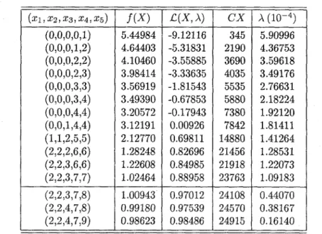
Let inj) = (2.1,1.5,1.2,5.0,3.5) and (cj) = (2980,1751,462,1500,345) and a budget of 6 = $25000. An exhaustive search finds the optimal at X* = (2,2,3,8,6) with
fix*) = 0.97502 and a cost of $24918. Table 1 provides the allocations generated
by the general marginal allocation algorithm starting from an initial kit containing no spare parts. As can be seen in Table 1, {/(X*^)} and {Afc} are decreasing sequences, {£(X'^, Afc)} is an increasing sequence, consequently {X^} is a sequence of undominated allocations. The algorithm delivers (2,2,3,7,7) without employing Corollary 1 or the optional step. These are solutions given above the horizontal line in Table 1. If Corollary 1 is invoked, the sequence of solutions generated is given below the horizontal line and the allocation (2,2,4,7,9) is delivered as a near optimal solution with fiX) = 0.98623 and a cost of 24915. This is also an upper bound for the value of the objective function. A lower bound is also produced by using Theorem 4, and the lower bound is at (3,2,3,7,7) with /(X) = 0.75561 and a cost of 26743.
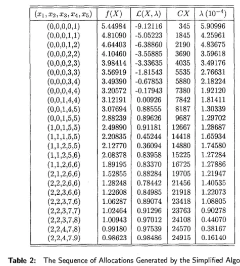
Table 2 gives the sequence of allocations generated by the simplified marginal allo-cation algorithm by using the optional step as well. Both algorithms converge to the same solution.
The allocation (2,2,2,6,6) is obtained from the allocation (1,1,2,5,5) after one iteration by using the general marginal allocation algorithm without the use of Theorem 3, as seen in Table 1. The combination of components is given hy W = (1,1,0,1,1) and the multiplier A = 1.28531 x 10-^. The simplified algorithm generates the allocations (1,1,2,5,6), (1,1,2,6,6), (2,1,2,6,6) and finally (2,2,2,6,6) starting from (1,1,2,5,5). It is easy to notice that this multiplier is expressed as a linear combination of the multipliers generated for the intermediate solutions in Table 2. (The Uj values are the A values generated by the simplified algorithm.) The cost of the combination W = (1,1,0,1,1) is CW = 6576. As an illustration of Theorem 2, it is easy to observe that
= Ej=i icj/CW)i^j at the solution (2,2,2,6,6).
10, - 4
(1.27284(345) -f 1.27886(1500) -I-1.21947(2980) -I-1.40535(1751)) = 1.28531 x 10- 4 6576
An illustration of the results of Corollary 1 is presented here. At the point X = (1,1,2,5, 5), the vector (r^) of marginal values per unit of each component is given by (1.04125,0.85596,0.53834,1.24375,1.27284)(10'^) The rankings of the TJ values gives '''5 ^ '''4 ^ Ti > r2 > r3. The marginal algorithm in Table 2 first adds one unit of component 5 to the current solution to obtain (1,1,2,5,6). Then the vector (r^) = (1.08240,0.89569,0.56763,1.27886,0.53066)(10-^) is obtained. At the point X + eg, r4 is the largest as indicated in the Corollary 1, and the new allocation (1,1,2,6,6) is ob-tained. This time the vector (r^) = (1.21947,1.02443,0.65990,0.72280,0.59931)(10"^) has ri as the largest marginal value and the new allocation is (2,1,2,6,6). Consequently, the vector (r^) = (0.62648,1.40535,0.94671,0.89944,0.79397)(10-^) is obtained and r^ is the largest now to yield the allocation (2,2,2,6,6). Prom this point on, the linear combination A = X^ • CjVj/CU is smaller than A^ = 1.28531 x 10~^ for all other U. Hence, (2,2,2,6,6) is delivered as an undominated solution.
(xi,X2,a::3,2;4,a;5) (0,0,0,0,1) (0,0,0,1,1) (0,0,0,1,2) (0,0,0,2,2) (0,0,0,2,3) (0,0,0,3,3) (0,0,0,3,4) (0,0,0,4,4) (0,0,1,4,4) (0,0,1,4,5) (0,0,1,5,5) (1,0,1,5,5) (1,1,1,5,5) (1,1,2,5,5) (1,1,2,5,6) (1,1,2,6,6) (2,1,2,6,6) (2,2,2,6,6) (2,2,3,6,6) (2,2,3,7,6) (2,2,3,7,7) (2,2,3,7,8) (2,2,4,7,8) (2,2,4,7,9)
fiX)
5.44984 4.81090 4.64403 4.10460 3.98414 3.56919 3.49390 3.20572 3.12191 3.07694 2.88239 2.49890 2.20835 2.12770 2.08378 1.89195 1.52855 1.28248 1.22608 1.06287 1.02464 1.00943 0.99180 0.98623£iX,x)
-9.12116 -5.05223 -6.38860 -3.55885 -3.33635 -1.81543 -0.67853 -0.17943 0.00926 0.88555 0.89626 0.91181 0.45244 0.36094 0.83958 0.83370 0.88284 0.78442 0.84985 0.89074 0.91296 0.97012 0.97539 0.98486CX
345 1845 2190 3690 4035 5535 5880 7380 7842 8187 9687 12667 14418 14880 15225 16725 19705 21456 21918 23418 23763 24108 24570 24915 A (10-4) 5.90996 4.25961 4.83675 3.59618 3.49176 2.76631 2.18224 1.92120 1.81411 1.30339 1.29702 1.28687 1.65934 1.74580 1.27284 1.27886 1.21947 1.40535 1.22073 1.08805 0.90278 0.44070 0.38167 0.16140Table 2: The Sequence of Allocations Generated by the Simplified Algorithm
The relative error in this example is 1.15%. The allocation (2,2,4,7,9) with fiX) = 0.98623 and CX = 24915 is generated by the algorithm and one additional step by
n 5 10 20 30 40 50 60 70 80 90 3.5 X time 0.164 1.036 6.702 21.282 47.562 95.550 153.100 258.322 384.952 519.812 std. 0.039 0.185 0.947 3.210 6.290 6.140 6.264 16.827 7.425 22.487 Budget Level 5xEcj time 0.176 1.320 8.526 28.042 65.076 127.866 207.126 333.750 513.366 700.914 std. 0.046 0.234 0.989 3.387 5.456 6.884 9.566 4.524 10.815 22.892
7xEc,-time 0.240 1.636 10.798 37.724 83.760 163.582 267.586 434.000 657.328 913.682 std. 0.050 0.279 1.110 7.477 5.974 6.301 13.930 10.811 18.073 24.397 Table 3; Results of Numerical Experimentation (in seconds)maXj{{fiX) - fix + Cj))/cj} yields the solution (2,2,4,7,10) with CX = 25260 and fix) = 0.98440. Eventhbugh the cost of this solution exceeds the budget, this solution
does not form a lower bound for the value of objective function. This also implies that expression (39) can not be relaxed or changed. Several randomly chosen problems are run to observe the relative efficiency of the method and the allowable relative percentage error as the difference between the upper and lower bounds on a 486 based PC. The mean failure rates ifXj) come from a uniform distribution over the interval (0.5,9.5) and the costs {cj) are obtained from a uniform distribution over the interval (150,3000). The budget level is also changed to observe the effect on the computation time and the relative eiTor. The budget level is set to 3.5 E Cj or 5 E Cj or 7 E Cj during the numerical experimentation. As the budget level increases, intuitively more allocations need to be generated. Average computation times in seconds for various size randomly generated problems are summarized in Table 3. For problems with n = 5, the optimum solutions are obtained by an exhaustive search to observe the accuracy of the algorithm. 60% of the solutions obtained by (MAA) marginal allocation algorithm for problems of size 5 happen to be optimal. The MAA takes, on the average, 0.166 seconds, 0.176 seconds, and 0.240 seconds to reach a (near) optimal solution for problems with n = 5 and b = 3.5E^j, b = 5'^Cj., b = 7 E c j respectively. The exhaustive search process takes on the average 91.838 seconds, 298.006 seconds, 816.128 seconds for the same problems respectively. The relative error is 0.397%, 1.599%, and 1.755% for the same set of problems respectively.
The allowable relative error is about 6% for problems with n == 10 irregardless of the budget size. If ra == 20 or ra = 30, then the allowable relative error falls to 1.583%. If n = 40 or 72 = 50, the allowable relative error remains around 0.797%. For larger size problems (n > 60), the allowable error stabilizes and remains around a mean of 0.398% with a standard deviation of 0.170%.
The execution time as indicated by the numerical experimentation is a function of the number of components and the budget level. A regression analysis shows that the execution time can be expressed as i = 0.00056n^'^4394^o.7452^ j^Yie variability is very low as can be noticed from the relatively low standard deviations in execution times in Table 3.
0 1 2 3 4 5 6 7 8 0 2.71305 2.15734 1.81040 1.62784 1.54621 1.51478 1.50422 1.50108 1.50025 1 2.46673 1.73542 1.23117 0.94339 0.80620 0.75065 0.73122 0.72526 0.72364 2 2.35656 1.52266 0.91998 0.56365 0.38929 0.31731 0.29175 0.28382 0.28164 3 2.31631 1.43765 0.79027 0.40208 0.21020 0.13040 0.10191 0.09303 0.09058 4 2.30405 1.40999 0.74679 0.34718 0.14896 0.06631 0.03674 0.02752 0.02497 5 2.30088 1.40245 0.73469 0.33176 0.13168 0.04819 0.01831 0.00898 0.00640 6 2.30017 1.40069 0.73183 0.32808 0.12754 0.04385 0.01389 0.00453 0.00195
Table 4: Function Values of
6. CONCLUSIONS
Marginal allocation algorithm is a simple and easy to implement procedure in obtaining a (near) optimal solution to discrete allocation problems. The combination of items that yields the largest marginal value per unit is added to the allocation. If the Lagrangian function is discretely convex, the marginal allocation algorithm generates a sequence of undominated allocations. The method is simplified and reduced to the case of traditional marginal allocation algorithm. An implication of this result is that the marginal value per unit of each item, instead of the marginal value of a combination of several items jointly, can be used in converging to a (near) optimal allocation. Further, a lower bound is obtained by using the algorithm. The case of separable functions is shown to be a special case.
A real life example is presented to illustrate the implemetation of the method. Nu-merical expreience has shown the efficiency of the method and the quality of the solutions Obtained.
Single constraint allocation problems occur in real life and and as subprobiems to more complex problems. EfEcient solution procedures are of importance to this class pf problems. This research presents an efficient procedure for a class of problems with nonseparable objective functions and a linear constraint or conversely. A major contri-bution of this research is to prove that the marginal allocation algorithm can generate undominated solutions for this class of problems. A further potential research area is an adaptation of this method to problems with both nonseparable objective function and constraint.
Appendix
A Summary of Discrete Convexity
Let 5 C /!f of n-tuples of nonnegative integers, a function for sAlx,y e S and at G (0,1),
acpix) + (1 — a)(j>iy) > min i
: S —^ R is discretely convex if, (42) wbere N(z) = {u e S \ z = ax + il - a)y, \\u - z\\ < 1} and ||M|| = maXj{JMj|}. This is a ratber straight forward extension of tbe definition of convexity for continuous functions to tbe discrete functions. Tbe restriction of any continuous function does not necessarily yield a discretely convex function as sbown by Miller (1970,1971), and Yuceer (1995). Only a weigbted continuous convex function yields a discretely convex function wben restricted to a discrete space.
a;2\xi 0 1 2 3 4 5 6 0 2.71305 2.22932 1.95436 1.84378 1.83413 1.87468 1.93610 1 2.68267 2.02334 1.59107 1.37527 1.31006 1.32649 1.37904 2 2.78844 2.02652 1.49582 1.21147 1.10909 1.10909 1.15551 3 2.96413 2.15745 1.58205 1.26584 1.14594 1.13812 1.18161 4 3.16781 2.34573 1.75451 1.42688 1.30064 1.27185 1.33238 5 3.38058 2.55413 1.95835 1.62740 1.49930 1.48779 1.52989 6 3.59581 2.76831 2.17143 1.83966 1.71110 1.69939 1.74141
Table 5: Values of the Lagrangian with A = 0.07198
a;2\a;i 0 1 2 3 4 5 6 0 2.71305 2.29453 2.08478 2.03941 2.09497 2.20073 2.32736 1 2.87830 2.28418 1.91712 1.76653 1.76653 1.84817 1.96593 2 3.17970 2.48299 2.01750 1.79836 1.76119 1.82640 1.93803 3 3.55102 2.80955 2.29936 2.04836 1.99367 2.05106 2.15976 4 3.95033 3.19346 2.66745 2.40503 2.34400 2.38042 2.50616 5 4.35873 3.59749 3.06692 2.80118 2.73829 2.79199 2.89930 6 4.76959 4.00730 3.47563 3.20907 3.14572 3.19922 3.30645
Table 6: Values of the Lagrangian with A = 0.13719
Let D be a convex hull of the discrete space S. A function 4> : D -^ R is weighted at any point X e D if there exists weights Wxiu) for all u 6 A''(a;) such that (l>ix) = Eu6W(x) Wxiu)(t>iu). The weights Wxiu) satisfy the conditions that Eue.w(x) '^^i''^) = ^ ^^^d Wxiu) > 0.
A discretely convex function has its local minimum as the global optimum. The first forward differences of a discrete function is defined as Aj4>{x) = (f>ix + ej) - 4)ix) for all j = 1, 2 , . . . , n A discretely convex function has its first forward differences increasing or at least nondecreasing. The commonly used definition of convexity for a discrete function in the literature, see Denardo (1982), Fox (1966), for instance, is that the first forward differences of each component are nondecreasing. The equivalency of this common definition to the discrete convexity is shown in Yuceer (1995). If a separable function /i(X) = E"=i ^^A^i) is discretely convex, then it has necessarily nondecreasing first forward differences which can be shown very easily. At the points X and X -|- 2et for 1 < i < n and for any a G (0,1), the following statement holds by the discrete convexity.
-f (1 - a)hiX + 2et) =
+
+ (1 - a)htixt + 2) > /i(w) (43) In particular, the above statement (43) holds for a = 0.5, then the set Niz) contains only one element, namely ( n , a;2,..., at -M,...,Xn). Thus the following equality (44) holds now.h{u) = (44)
Consequently, 0.5htixt) + 0.5htixt + 2) > htixt + 1) and this relationship in turn implies that . htixt + 2) - htixt + 1) > htixt + 1) - htixt) or equivalent^ Ahtixt + 1) > Ahtixt) for any t = 1,2,... ,n. The proof of the converse of this statement requires showing the existence of a weighted continuous convex function for any discrete function with nondecreasing first forward differences.
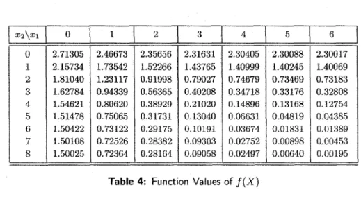
As a demonstration of discrete convexity, the function f{X) — J ^ ^ Q ( 1 — n " _ i Pji^j H-/c)) with n = 2, (/ij) = (1.5,2.3) and (cj) = (3,1) is considered. The values of f{X) are given in Table 4 and Tables 5 and 6 gives the values of the Lagrangian for A = 0.07198 and A = 0.13719 respectively. The Lagrangian function is discretely convex with both multipliers. It should be noticed here that the function f{X) is also discretely convex corresponding to the case of A = 0 in the Lagrangian function.
The discrete convexity is a weaker condition than the weak concavity (convexity) defined by Federgruen and Groenevelt (1986). Their condition (R3) states that if j/ >R X, and xi = yi then x-\-ei >R x-\-e2 implies y-\-ei >R y + e^. The function f{X) does not obey the rule (R3) as illustrated below. Consider the points (2, 2) and (2, 6). From the Table 4, /(3, 2) = 0.79027 and /(2,3) = 0.56365 then /(3,2) > /(2,3). On the other hand, /(3,6) = 0.10191 and /(2,7) = 0.28382 but /(3,6) < /(2,7).
Tables 5 and 6 illustrate some of the statements used in the proof of Theorem 3. In Table 5, the minimum of the Lagrangian occurs at the points (2,4) and (2,5) and £{2,4) = £(2, 5) = 1.10909. This illustrates the fact that a multiplier A exists always for a discretely convex function to make the points y and y -{• et for some t the minimum. It is also easy to observe that the minimum of a discretely convex function can be shifted from one point to another point in the neighborhood of the former point by an appropriate choice of the multiplier A, as illustrated in Tables 5 and 6.
REFERENCES
1. S. Brumelle, D. Granot, "The Repair Kit Problem is Revisited", Operations Research, Vol. 41, No. 5, pp. 994-1006, 1993.
2. A. Dechter, R. Dechter, "The Greedy Solution of Ordering Problems", ORSA Journal on Computing, Vol. 1, No. 3, pp. 181-189, 1992.
3. E.V. Denardo, Dynamic Programming: Models and Applications, Prentice-Hall, Engle-wood Cliffs, New Jersey, 1982.
4. K.-H. Elster (editor). Modem Mathematical Methods of Optimization, Akademi-Verlag, Berlin, 1993.
5. H. Everett, "Generalized Lagrange Multiplier Method for Solving Problems of Optimum Allocation of Resources", Operations Research, Vol. 11, pp. 399-417, 1963.
6. A. Federgruen, H. Groenevelt, "The Greedy Procedure for Resource Allocation Problems: Necessary and Sufficient Conditions for Optimality", Operations Research, Vol. 34, No. 6, pp. 909-918, 1986.
7. A. Federgruen, P. Zipkin, "Solution Techniques for Some Allocation Problems", Mathe-matical Programming, Vol. 25, pp. 12-24, 1983.
8. B. Fox, "Discrete Optimization Via Marginal Analysis", Management Science, Vol. 13, No. 1, pp. 210-216, 1966.
9. T. Ibaraki, N. Katoh, Resource Allocation Problems, The MIT Press, Cambridge, Mas-sachusetts, 1988.
10. E.P. Kao, "On Incremental Analysis in Resource Allocations", Operational Research Quarterly, Vol. 27, pp. 759-763, 1976.
11. B.L. Miller, Unconstrained Optimization in Integers, The RAND Corporation, Santa Monica, California, RM-6165-PR, January 1970.
12. B.L. Miller, "On Minimizing Nonseparable Functions Defined Over the Integers With an Inventory Application", SI AM Journal of Applied Mathematics, Vol. 21, No. 1, pp. 1-15, 1971.
13. S.S. Nielsen, S.A. Zenious, "Massively Parallel Algorithms for Singly Constrained Convex Programs", ORSA Journal on Computing, Vol. 4, No. 2, pp. 166-181, 1992.
14. U. Yuceer, "Discrete Convexity", technical report, Bilkent University, Ankara, Turkey, April 1995.
15. P. Zipkin, "Simple Ranking Methods for Allocations of Resources", Management Science, Vol. 26, No. 1, pp. 34-43, 1980.
Umit Yuceer is currently affiliated with Bilkent University, Ankara, Turkey, after having worked for several universities in Canada. He has a Ph.D. in Industrial Engineering and Management from Oklahoma State University. His research interests include operations research, transporta-tion/distribution, marginal analysis, and integer programming. He has research articles published in European Journal of Operational Research and research and/or tutorial articles published on reliability.