Reducing demand signal variability via a quantitative fuzzy grey regression approach

Customer Customer Supplier Supplier Manufacturer Manufacturer External Complexity Internal Complexity Total Complexity Material Information Supplier External Complexity

Reducing Demand Signal Variability via a Quantitative Fuzzy Grey Regression Approach

Hakan TOZAN, Mumtaz KARATAS, Ozalp VAYVAY

Abstract: The total system performance of dynamic and complex supply chain networks depends mainly on accurate demand signal estimation as incorporated with an

appropriate decision-making process. Due to the field of activity and architecture, however, it is hard to choose a proper forecasting and demand decision model that would befit the complexity of the system. This paper develops a conjoint intelligent hybrid system, comprised of an adaptive neuro-fuzzy inference system (ANFIS) based demand decision process, integrated with crisp grey GM (1,1) and fuzzy grey regression (FGR) forecasting models. We adopt this approach in an attempt to reduce the demand signal variability in supply-chain networks and to evaluate the system response to the proposed models under predefined, relatively low, medium and high demand signal variations. The results obtained from the simulation runs illustrate that the proposed hybrid system reduces the variability considerably; and also, could be considered as a substantial tool for reduction of supply chain phenomenon so called Bullwhip effect.

Keywords: ANFIS; demand signal processing; fuzzy forecasting; fuzzy logic; grey systems 1 INTRODUCTION

In recent years, Supply Chain Networks (SCNs) have attracted a great deal of attention since the dynamic and chaotic structure of those networks aims at satisfying customer needs which include sophisticated interrelated functions and processes. The management of these complex structures also directly influences the compaction power of companies and even countries in both civilian and military domains [1, 2].

In addition to their far too numerous components with many interactions and dependencies, major triggers of the complexity in SCNs could generally be stated as material and information flows with highly uncertain natures. This complexity can be classified under three groups as internal, external and total complexity representing the interactions via material and information flows within the internal players, between internal and external players and

throughout all SCN as illustrated in Fig. 1 [3]

Figure 1 Complexity flow [3]

The system performance of SCNs directly depends on accurate, on-time and appropriate information flow through the whole chain [2, 4, 5]. Thus, demand signal (DS) estimation incorporated with decision-making processes is a crucial activity, which has to be performed and designed precisely to maintain and improve

supply-chain performance. Although the importance of a DS for forecasting and decision-making processes performed in every stage of SCN is beyond our argument, the determination of an appropriate forecasting and decision-making model that will fit the DS pattern is a difficult problem, as the vital data varies according to the activity field and SCN structure. Just at this point, the "Bullwhip or Whiplash Effect" (BWE), a well-known phenomenon of DS in SCNs, emerges as a serious problem to cope with [5, 6]. BWE, which arises from the chaotic nature of SCNs, is simply the variability of the DS between the SCN stages. Additionally, an increase in this variability as DS moves upstream from the customer to the consequent stages of the SCN, triggers undesirable excess inventory levels, overload errors in production activities, defective labor force, increases in costs, etc. The major causes of BWE have been reported in the previous studies as follows: irrational decision-making process, DS forecast updating, order batching and price fluctuations [5-14].

There exists a broad literature about BWE in SCN topics; but, despite this broad literature studies that involve fuzzy approaches to that phenomenon such as Carlsson et al. [15, 16], Wang et al. [17, 18], Efendigil et al. [19] are relatively few in literature, which also is the main motivation of this paper.

This paper, rather than assessing the impacts of all causes, specifically focuses on the first two relatively controllable issues: the decision-making process and DS forecast updating. A conjoint hybrid system composed of an adaptive neuro-fuzzy inference system (ANFIS) based demand decision process integrated with Grey GM (1,1)/fuzzy grey regression (FGR) is proposed. Furthermore, the response of BWE to the proposed system in a stage SCN under relatively low, medium and high DS variations is analyzed by quantifying BWE.

The paper is organized as follows: section 2 is reserved for the basic idea of ANFIS. In section 3, the forecasting models used in the paper are presented. Section 4 introduces the proposed simulation model and DS pattern with ANFIS and BWE quantified for the measurement and the comparison of the results. In section 5, the results obtained from the simulation runs are compared with the basic crisp model. Finally, we highlight conclusions and potential future works in section 6.

2 ADAPTIVE NEURO-FUZZY INFERENCE SYSTEM (ANFIS)

As being one of the well-known hybrid intelligent systems, the neuro-fuzzy systems (NFSs) can be described as the combination of two different methodologies: artificial neural networks (ANNs) and fuzzy logic (FL). This integrated methodology is capable of learning, generalizing, adapting and parallelism, which basically come from ANN abilities, and deducing knowledge from a set of given rules that also comes from the fuzzy inference systems (FISs). Therefore, using such a system improves the reliability of both FL (i.e., no ability to learn, difficulties in parameter tuning and developing suitable membership functions) and ANN (i.e., black box, difficulties in deducing knowledge) by covering their weak sides with the powerful abilities of robust methodologies.

The aim of ANFIS in the learning process is to adjust the premise (initial parameters) and consequent parameters till obtaining the desired input-output mapping from the FIS. This learning task is attained by integrating two techniques: (1) the least squares method (LSM), and (2) the gradient descent method (GDM). The integrated approach consists of forward and backward passes. In specific, at the forward pass, while the premise parameters in Layer 1 are kept constant, functional signals proceed towards the Layer 4. Next, the consequent parameters in Layer 4 are determined with the utilization of the LSM. At the backward pass, on the other hand, the error measure propagates backward while consequent parameters are kept constant. At this stage, the premise parameters are updated with the utilization of GDM which adjusts the membership functions [20, 21].

3 GREY GM (1,1) AND FUZZY GREY REGRESSION FORECASTING

In every field of science, engineering and management almost all planning and decision activities directly depend on predicting future. However, determining the appropriate technique and its application to the systems is not an easy activity as the nature of prediction comprises uncertainty or vagueness [22]. At this point, due to their capability of providing intermediate values between the expressions mathematically, FL and fuzzy set theory are the best ways to model uncertainty and vagueness [2, 4, 22-27].

Contrary to similar cases involving human judgment, crisp sets will subgroup the given discourse universe into two: members are affixed to the set with certainty and those which are not. This separation arises from their mutually exclusive structure, and leads the decision maker into setting an absolute boundary between the decision variables and the alternatives thereof. As introduced by Zadeh [24], the key difference lies in the capability of FL to process data via partial set membership functions [4, 23, 25-27].

As the main problem in SCN is to handle the uncertainty, Grey GM (1,1) and FGR models are used in the study as they are both concerned with the systems comprising uncertainties and lack of sufficient amount of information. As might be expected, the ‘grey’ here represents information laying between totally clear and the

totally unknown layers which could be described as the information within the foggy or fuzzy layer [2, 37].

In the following parts of this section Grey GM (1,1) and Fuzzy Grey Regression forecasting are explained in the light of Wang [37], Zhang [38], Tsaur [39,40], Tozan and Vayvay’s [2] studies. In contrasts to other statistical forecasting techniques, which mostly require large amounts of data sets pertaining to previous periods, the grey theory utilizes the accumulated generating operation (AGO) in order to attain regularity and reduce noise by converting ambiguous original time series data to monotonically increased data series [41]. AGO is an important operation in the concept of grey system theory since it allows converting raw (unimproved) stochastic data to useful regular series data. The inverse accumulated generic operation (IAGO), on the other hand, is another important tool used in the grey system theory, to transform AGO generated regular series to raw data. The main objective of the grey model is to generate regular differential equations by using AGO in the general form as GM (n, m) where n and m denote the order of ordinary differential equation, and the number of grey variables which define the order of AGO and IAGO, respectively. It should be noted that an increase in n and m leads to an exponential increase in the required computation time. The most commonly-used model in the grey system theory is GM (1,1) since it requires smaller data sets and lower computation time [2, 38].

The Grey GM (1,1) model basically targets to attain the internal regularity for the available past data which will later be used to forecast and transfer the arranged sequence

into a differential equation. Let the vector D0 _{denote the}

data of n elements collected from the system. We can express it as follows:

0 0 0 0 0

1 2 3

( , , ,..., _n)

D = D D D D (1)

Then, the AGO series generated by using D0 _{is represented}

by D1 _{as follows:}

1 1 1 1 1

1 2 3

( , , ,..., )n

D = D D D D (2)

In Eq. (2), the kth _{data is calculated as} 1 0

1 , k k i i D =

∑

∀ = Note that the data for accumulated

generating sequence increases monotonically. If a GM (n, m) model is adopted, and it is not possible to achieve regularity with one AGO, then the operation has to be repeated m times until the data set becomes more regular.

A first-order differential equation to establish internal

regularity for D1 _{is given in Eqs. (3) and (4). Note that since}

D1 _{increases monotonically, it can be approximated by an}

exponential function that has the dynamics of a first-order differential equation. 1 1 d d D _{aD b} k + = (3) 1 1 1 0 d _lim d h k h k D D _D k → + h   = _ − _  ; ∀ ≥k 1 (4)

In Eq. (3) 𝑎𝑎 and 𝑏𝑏 denote the developed coefficient and the grey control variable, respectively. If sampling interval

is set to one unit, i.e. h = 1, then the first derivative of D1

can be expressed as a discrete time series:

1 1 1 1 1 0 1 1 1 d d k 1k k k k D D _{D D D D} k + + +   =_ − _= − =   ; ∀ ≥k 1 (5)

Next, the second part of the grey model, 1

average

D can be

stated in the matrix form as follows:

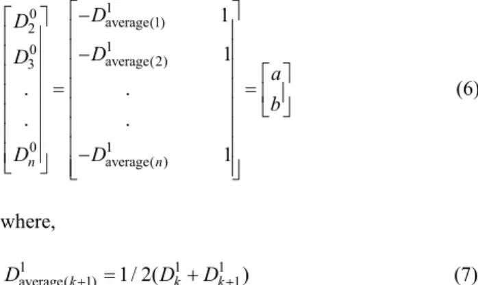
1 0 _average(1) 2 1 0 average(2) 3 0 1 average( ) 1 1 . . . . 1 n n D D D D a b D D ₋        −     _{  }  _{ = =}      _{ }         ₋      _ _ (6) where, 1 1 1 average( 1)k 1/ 2( k k 1) D + = D +D+ (7)

Applying LSM in Eq. (3), the coefficients a and b can be calculated as follows:

( )

1 1 2 1 1 1 3 2 1 1 1 0.5( ) 1 0.5( ) 1 . . . 0.5( n n ) 1 D D D D B D D− − +    − +       =       _{− +}    (9) 0 0 0 0 2, ,..., 3 n D _{= }D D D _{ (10)}

where n denotes the cardinality of data set used and _D0_is

the raw sequenced data.

Using coefficients a and b, Eq. (2) can also be

estimated by the value Dˆ1k+1. The output forecast for period

k + 1, Fˆk0+1, can be calculated with equations (11) and (12),

respectively.

(

)

Though the fuzzy model of Grey GM (1,1) performs successfully in systems with chaotic and dynamic nature like SCNs, the input data of the model have to be fuzzy

which restricts the usage of the model for the complete crisp systems. A fuzzification for the input data has to be employed before initializing the model. However, the determination of the appropriate membership functions for the demand data is not an easy activity since the characteristics of the demand data are generally unknown. Therefore, FGR models overcome this problem by utilizing fuzzy regression models, which have the ability to apply crisp input data. FGR model proposed by Tsaur [40] is a relatively simple hybrid model using fuzzy set theory and grey GM (1,1) model. The model evaluates the fuzzy relations between dependent and independent variables granulating a concept into a set of membership functions. The input data for the model can also be fuzzy. In this paper, we use and discuss the system for crisp input and fuzzy output proposed by Tsaur [40] (see 37 for details of the model).

4 PROPOSED SIMULATION MODEL AND ANFIS BASED DECISION PROCESS

The simulation method stands as the most preferable of all options viable to analyse systems like SCN. This section provides a simulation model based on a near beer distribution game [3, 11-13, 42, 43], extended with ANFIS, Grey GM (1,1) and FGR: an improvement over the original Sterman beer game [3, 11-13] and over Paik’s interpretation [44] incorporating inventory/capacity restriction and specific delay functions.

The material and information flow in beer are described in Fig. 2. MATLAB is used as the simulation tool to simulate a two stage SCN for evaluating the response of DS variability to the proposed system. The game attempts to oversee every stage of the supply-chain so as to ensure sufficient inventory to meet the demand that results from the predecessor stage, acting upon a limited flow of supply line information to minimize total cost by avoiding stock out [44]. DISTRIBUTOR WHOLESALER RETAILER FACTORY ORDER ORDER ORDER CUSTOMER ORDER GOODS GOODS GOODS SIGNAL DELAY

(SIGNAL DELAY) (SIGNAL DELAY)

SIGNAL(DELAY

SIGNAL (DELAY) SIGNAL DELAY

SIGNAL DELAY

SIGNAL (DELAY)

GOODS

Figure 2 Material and information flow in beer

The key features increasing the involved criteria and accordingly the real-world applicability of the game include limited availability of information as well as delayed flows of information and shipment.

Order and production decision processes in each stage of the simulation are simple and include the following factors: current demand, actual inventory level, desired inventory level, actual pipeline orders (actual supply line), desired pipeline orders (desired supply line) and demand

forecast [3, 11-13, 44]. The ordering/ production decision process can be formulized as [3, 11-13, 44, 45]:

[

]

(

)

t t t t

O Max= F + IC SlC+ (13)

where Ot is the order quantity, Ft is the forecast value, ICt

is the correction of inventory and SlCt is the correction of

supply line in period t which is explained with the following formulations: ( ) t I t t IC =θ DInv Inv− (14) ( ) t Sl t t SlC =θ SD SA− (15) 1 (1 ) 1, 0 1 t t t F =α OI₋ + −α F₋ ≤ ≤α (16)

Where: DInvt - the desired inventory level, Invt - the current

(actual) inventory level, SDt - the desired supply line, SAt -

the current (actual) supply line, θI and θSl - the adjustment

parameters of inventory and supply line respectively, OIt−1

- the actual value of the orders received (incoming orders) in period t − 1, α - the smoothing constant.

Both θI and θSl will determine the emphasis placed on

the variance the desired and actual values inventory and supply line [44]. In this light, a disturbance term ε for each period and parameter β can be defined as follows, enabling recoding of the overall decision rule:

[

]

(

)

The minimum, mean, and maximum values of the parameters of the decision rule are estimated by Sterman [3, 11-13] and summarized in Tab. 1.

Table 1 Estimated Parameters [11]

Parameters α θSl β Al'

Minimum 0.00 0.00 0.00 0.00

Mean 0.36 0.26 0.34 17

Maximum 1.00 0.80 1.05 38

As stated before, the analyses are made for a two-stage SCN system consisting of customer, retailer, and factory. In the following part of the system structure and the formulation of the base model are defined for any time period t at retailer and factory stages where the production for the whole system is made. The first decision rule of all stages can be redefined with respect to (17) and (18) as in (19) below:

(

)

O Max F DInv Inv

SD SA θ θ β − − − − −  = _ + − +  + − _ (19)

where subscript i = 1, 2 stands for the stage concerned (i.e.

1→R, 2→F, where R and F denote retailer and factory

respectively). The whole formulation for a general stage is given in Eqs. (19)-(33). , , , i t i t i t IS =OS DLs (20) , , 1 ( , ,) i t i t i t i t Inv =Inv − + IS −OS (21) , , 1 ( , ,) i t i t i t i t OB =OB − + IO −OS (22) , , , , , if othewise i t i t i t i t i t OB Inv OB OS Inv ≥  =   (23) , , i t i i t DInv =Sc F× (24) , , , i t i t i t SD =F ×DL (25) , , , i t i t i t OO =O DLo (26) , , 1 ( , ,) i t i t i t i t IPo =IPo − + O −OO (27) 1, , , i t i t i t IO+ =OO DLm (28) , , 1 ( , , ) i t i t i t i t IPm =IPm − + OO −IO (29) , , 1 ( , , ) i t i t i t i t IPs =IPs − + OS −IS (30) , , , , , i t i t i t i t i t

SA =IPo +IPm +IPs +OB (31)

(

)

P Max F DIinv Inv

SD SA θ θ β − − − − −  = _ + − +  + − _ (32) , , , if . if othewise F t F t F t P Fc P FP Fc ≥  =   (33)

Where: IS - the incoming shipment (shipments received);

OS - the outgoing shipment (shipments released); DLs - the

delay in shipment (time required for a shipped item to reach the destination which can be defined as a variable or a constant depending on the decision-maker and analysis that will be performed); OB - the orders backlogged (cumulative sum of orders that have been received but not have been met yet); IO - the incoming order (orders received); DL - the aggregate time delay for the stage which is the sum of time delays concerning shipment; DLs - paper work (i.e. office work); DLo and postal (i.e. mailing) DLm; OO - the outgoing orders rate directly related to the DLo and decided quantity of orders (O); IPo - the orders in process in paper work (i.e. clerical); IPm,

IPs - the quantities in process in mailing and shipment (i.e.,

orders that have been shipped but not received); P - the production decision quantity regardless of the factory capacity; Fc - the single period production capacity of the factory.

4.1 Proposed ANFIS Based Decision Process

System thinking is the base idea for an appropriate ordering (i.e., demand) decisions in SCN systems. Due to the chaotic and dynamic system of SCNs, decision-making process contains many parameters and variables that must be taken into account and in addition to those, the nature of decision-making; just like prediction, contains uncertainty and vagueness and also has to embrace the human judgment. Owing to these facts, the decision-making process of the SCN systems has to be determined attentively. To overcome these difficulties in decision-making process of SCNs, this study proposes an ANFIS based decision making process and aims to benefit from the capability of deduction from given rules (thanks to fuzzy inference system (FIS)), learning, generalization, adaptation and parallelism (thanks to ANN).

Different from the previous SCN simulations, the proposed model contains an ANFIS-based process in each SCN phase to set order quantities, based on FGR- and GM-based forecast values (1,1) and integrated with the inventory and pipeline data we used in the base model. We use MATLAB’s "Fuzzy Logic Tool Box" to build ANFIS structures, and again the same toolbox to find the solution. In ANFIS based demand decision process, Sugeno-type inference and the hybrid method is selected and used for the estimation of membership function parameters. The appropriate membership functions for the parameters are defined as Gaussian. The error tolerance is set to zero and ANFIS is trained for each selected forecasting model in stage with 200 training data with the given characteristics [4].

The inputs for each time period 𝑡𝑡 in each phase for the ANFIS based decision are as follows (i.e., the input neurons): (1) The demand forecast value for the upcoming period t + 1 (which is determined using grey GM

(1, 1) or FGR models), (2) Invt, (3) DInvt, (4) SAt, (5) SDt,

and (6) Oi−1,t. t OIi,t, Previous Incoming Order Information Compose Matrixes Generate AGO Series Compute a, b Determine

Crisp Forecast Value

Greey GM (1, 1) (Crisp) Crisp 0 ,D B  ˆ Compute the Forecast for 1 + t Crisp

Crisp Domain Crisp Domain

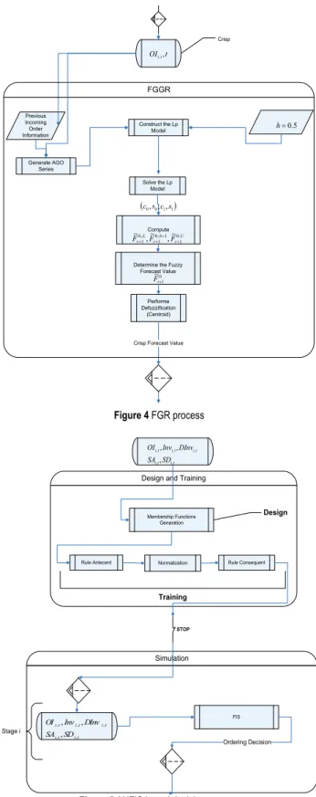
1 = t No Yes 1 1 ˆ + t D Figure 3 Grey GM (1,1) Process

Different from the base model’s decision-making process which uses the forecast value singly as an input and

once and again, as a parameter for determining the DInvt,

the proposed ANFIS based demand decision process does not duplicate the usage of forecast value in the decision process; which in fact helps to damp the BWE. Figs. 3, 4 and 5 illustrate the grey GM(1,1), FGR, ANFIS based decision process, respectively.

t OIi,t, Previous Incoming Order Information Solve the Lp Model 5 . 0 = h Construct the Lp Model Compute Performe Defuzzification (Centroid)

Crisp Forecast Value

FGGR Crisp (c0,s0;c1,s1) Generate AGO Series U t h t L t F F F 0, 1 1 , 0 1 , 0 1,~ ,~ ~ + = + +

Determine the Fuzzy Forecast Value 0 1 ~ + t F Figure 4 FGR process Rule Antecent Membership Functions Genaration

Normalization Rule Consequent

Design and Training t i t i t i t i t i SD SA DInv Inv OI , , , , , , , , Design Training STOP Simulation FIS t i t i t i t i t i SD SA DInv Inv OI , , , , , , , , Ordering Decision Stage i

Figure 5 ANFIS based decision process 4.2 Demand Signal Characteristics

Due to the aim of this study, the important characteristic of the DS is the variation. To capture the proposed model's performance against BWE, rather than the means of the generated DS, the standard deviation is changed from one simulation run to another and the means of DS fixed at a constant rate. The mean of the customer

DS;µ , is taken as 50 unit and three different standard _d

≤ σd < 15) variation, relatively medium (15 ≤ σd < 20)

variation, and relatively high (20 ≤ σd) variation in the

demand data.

The data sets representing demand information are assumed to be integer for all models and generated according to this assumption. Tab. 2 illustrates DS characteristics of the proposed simulation models.

Table 2 DS Characteristics of the proposed models

DS Distribution Normal

DS Mean (μd) 50 units

DS Standard deviations

σd

Relatively high 20 ≤ σd units

Relatively medium 15 ≤ σd < 20 units

Relatively low 10 ≤ σd < 15 units

4.3 Quantification of DS Variability (BWE)

DS variability (i.e., BWE) is quantified in one of the most common ways defining the phenomenon as a ratio of standard deviations of subsequent stages in two different ways considering the capacity options. For the simulation runs without factory capacity limits BWE is quantified as:

i i k

k

BWE↔ =_σσ i =1andk =2, 3 (34)

Where σ denotes the standard deviation of orders placed to upstream stage and subscripts {1, 2, 3} denote the customer, retailer, and factory, respectively. Defining the capacity limits as constraints for the production activities in the factory stage delusively reduce the variability and correspondingly the standard deviations. But this deceptive reduction does not actually illustrate the real intent of the decision process in factory as capacity directly limits the quantity of production. To overcome this misleading smoothness rising from the capacity limits and to evaluate the real rate of variability, BWE is expressed for simulation runs with factory limits as:

[

]

[

]

Although capacity limits defined for the factory (as discussed previously) ignoring the decision processes intent, delusively reduce the standard deviation values, in

the final evaluation of BWE values (i.e. BWETOTAL) for

each parameter combination, the same weights (i.e. the importance factor) are assigned to both results of the

simulation run with and without capacity limits. BWETOTAL

is computed as follows:

TOTAL Cap ₂ Uncap

BWE BWE

BWE = + (36)

Where BWECap represents the arithmetic mean of BWEC↔R

and BWEC↔F is obtained from the simulation runs with

factory capacity. BWECap represents the arithmetic mean

BWEC↔R and BWEC↔F obtained from the simulation runs

without capacity limits for the same parameter combinations under the same variation of the customer demand.

5 SIMULATION RESULTS

To make a realistic comparison between the base and proposed models, the base model simulations are performed for different values of the parameters in the decision-making process. The maximum, mean and minimum values of the parameters are used in the decision

rule of the base model. Finally, the safety constant Sc_i is

taken as five periods and delays: DLs, DLo, DLm and DLp, are assumed to be equal to 2 periods in each run.

The experiments of the base model are performed for all DS patterns: relatively low, relatively medium and relatively high. Furthermore, the different values for α, β and θ parameters are taken into account. In specific, eight different combinations exist for α equals 0.36 and 1, β equals 0.34 and 1.04 and θ equals 0.26 and 0.8 (for both with and without predefined capacity limit for factory). The results obtained from the simulation runs are

summarized in Tabs. 3-5. It is observed that BWETOTAL gets

the minimum value in the first combination (α = 0.36, β = 0.34, θ = 0.26) for relatively low, relatively medium and relatively high variations.

Based on these results, the proposed models are evaluated and compared with the base model with parameter combination -1- for all demand patterns concerned in this study with and without predefined capacity limit.

The results of the first proposed model, "hybrid Grey GM (1,1) and ANFIS Based Demand Decision Process" are illustrated in Table 6 whereas results obtained from the simulation runs of the second proposed model: "hybrid FGR and ANFIS Based Demand Decision Process", are summarized in Tab. 7.

When the results acquired from all simulation runs of the proposed model-1 are compared to those of the Base Model, the proposed model-1 has better performance than

the Base Model since BWETOTAL is found 3.342, 2.415 and

2.063 in the Base Model, and 1.225, 1.463 and 1.646 in the proposed model-1 for relatively low variation, relatively medium variation and relatively high variation respectively. Similarly, the proposed model-2 has better

performance than the Base Model since BWETOTAL is found

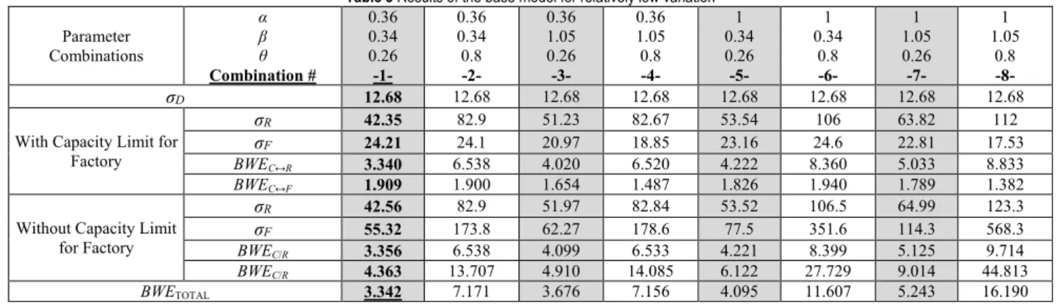
Table 3 Results of the base model for relatively low variation Parameter Combinations α β θ Combination # 0.36 0.34 0.26 -1- 0.36 0.34 0.8 -2- 0.36 1.05 0.26 -3- 0.36 1.05 0.8 -4- 1 0.34 0.26 -5- 1 0.34 0.8 -6- 1 1.05 0.26 -7- 1 1.05 0.8 -8- σD 12.68 12.68 12.68 12.68 12.68 12.68 12.68 12.68

With Capacity Limit for Factory

σR 42.35 82.9 51.23 82.67 53.54 106 63.82 112

σF 24.21 24.1 20.97 18.85 23.16 24.6 22.81 17.53

BWEC↔R 3.340 6.538 4.020 6.520 4.222 8.360 5.033 8.833

BWEC↔F 1.909 1.900 1.654 1.487 1.826 1.940 1.789 1.382

Without Capacity Limit for Factory σR 42.56 82.9 51.97 82.84 53.52 106.5 64.99 123.3 σF 55.32 173.8 62.27 178.6 77.5 351.6 114.3 568.3 BWEC/R 3.356 6.538 4.099 6.533 4.221 8.399 5.125 9.714 BWEC/R 4.363 13.707 4.910 14.085 6.122 27.729 9.014 44.813 BWETOTAL 3.342 7.171 3.676 7.156 4.095 11.607 5.243 16.190

Table 4 Results of the base model for relatively medium variation

Parameter Combinations α β θ Combination # 0.36 0.34 0.26 -1- 0.36 0.34 0.8 -2- 0.36 1.05 0.26 -3- 0.36 1.05 0.8 -4- 1 0.34 0.26 -5- 1 0.34 0.8 -6- 1 1.05 0.26 -7- 1 0.34 0.8 -8- σD 18.96 18.96 18.96 18.96 18.96 18.96 18.96 18.96

With Capacity Limit for Factory σR 49.58 91.43 56.55 92.37 63.71 121.5 72.87 139.9 σF 24.32 24.92 20.81 19.24 23.86 24.5 22.54 16.41 BWEC↔R 2.615 4.822 2.983 4.872 3.360 6.408 3.843 7.379 BWEC↔F 1.283 1.314 1.098 1.015 1.258 1.292 1.189 0.866 Without Capacity Limit for Factory

σR 49.77 91.31 57.34 92.65 63.89 122.5 74.21 140.9

σF 59.48 192.1 68.48 200.7 88.28 395.4 128.9 619.3

BWEC/R 2.625 4.816 3.024 4.887 3.370 6.461 3.914 7.431

BWEC/R 3.137 10.132 3.612 10.585 4.656 20.854 6.799 32.664

BWETOTAL 2.415 5.271 2.679 5.340 3.161 8.754 3.936 12.085

Table 5 Results of the base model for relatively high variation

Parameter Combinations α β θ Combination # 0.36 0.34 0.26 -1- 0.36 0.34 0.8 -2- 0.36 1.05 0.26 -3- 0.36 1.05 0.8 -4- 1 0.34 0.26 -5- 1 0.34 0.8 -6- 1 1.05 0.26 -7- 1 0.34 0.8 -8- σD 24.33 24.33 24.33 24.33 24.33 24.33 24.33 24.33

With Capacity Limit for Factory σR 56.15 100.5 61.94 102.9 73.46 137.6 82.41 158 σF 24.22 25.11 20.69 19.6 24.46 24.93 22.64 16.41 BWEC↔R 2.308 4.131 2.546 4.229 3.019 5.656 3.387 6.494 BWEC↔F 0.995 1.032 0.850 0.806 1.005 1.025 0.931 0.674 Without Capacity Limit for Factory

σR 56.48 100.5 63.17 103 74.15 139.5 84.28 159.6

σF 63.94 211.2 75.03 224.1 100.2 442.4 144.2 678.2

BWEC/R 2.321 4.131 2.596 4.233 3.048 5.734 3.464 6.560

BWEC/R 2.628 8.681 3.084 9.211 4.118 18.183 5.927 27.876

BWETOTAL 2.063 4.494 2.269 4.620 2.798 7.649 3.427 10.400

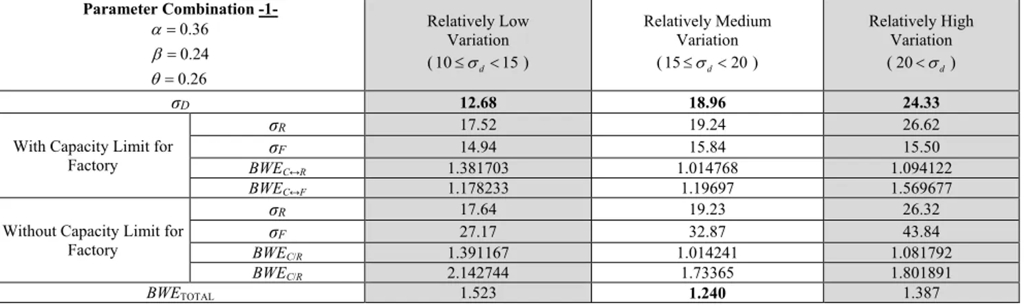
Table 6 Standard deviation and BWE results from the proposed Model-1 Parameter Combination -1- 0.36 0.24 0.26 α β θ = = = Relatively Low Variation (10≤σd<15) Relatively Medium Variation (15≤σd<20) Relatively High Variation ( 20<σd) σD 12.68 18.96 24.33

With Capacity Limit for Factory

σR 15.1 14.88 20.4

σF 9.292 9.279 9.328

BWEC↔R 1.191 1.274 1.193

BWEC↔F 1.365 2.043 2.608

Without Capacity Limit for Factory σR 15.1 14.88 20.4 σF 14.62 15.05 15.29 BWEC/R 1.191 1.274 1.193 BWEC/R 1.153 1.260 1.591 BWETOTAL 1.225 1.463 1.646

Table 7 Standard deviation and BWE results from the proposed Model-2 Parameter Combination -1- 0.36 0.24 0.26 α β θ = = = Relatively Low Variation (10≤σd<15) Relatively Medium Variation (15≤σd<20) Relatively High Variation ( 20<σd) σD 12.68 18.96 24.33

With Capacity Limit for Factory

σR 17.52 19.24 26.62

σF 14.94 15.84 15.50

BWEC↔R 1.381703 1.014768 1.094122

BWEC↔F 1.178233 1.19697 1.569677

Without Capacity Limit for Factory σR 17.64 19.23 26.32 σF 27.17 32.87 43.84 BWEC/R 1.391167 1.014241 1.081792 BWEC/R 2.142744 1.73365 1.801891 BWETOTAL 1.523 1.240 1.387 6 CONCLUSION

In this paper, a two-stage SCN simulation model (which is improved from the base simulation of Sterman [31-33] and its revised version of Paik’s [41], that includes inventory/capacity restrictions and specific delay functions) with ANFIS decision making process, Grey GM (1,1) and FGR forecasting models are used to simulate a two stage SCN for evaluating the response of DS variability to the proposed systems using MATLAB as the simulation tool. A comparison is carried out between the results "best results" obtained from the base model (for all combinations of different parameter values with and without capacity limits) and the results acquired from the proposed models using the same input values (with and without capacity limits) for relatively high, medium and low DS variations which are determined with the DS standard deviations. For each comparison between the base and the proposed models, BWE is quantified for each stage as a ratio of standard deviations of subsequent stages to reflect the amount of variability. The results showed that the proposed hybrid models considerably reduce BWE.

Based on the findings of this study, future studies can be performed using a full fuzzy simulation model with more than two stages in which DS variability is also determined with fuzzy statistics.

7 REFERENCES

[1] Chandra, C. & Kumar, S. (2000). Supply chain management in theory and practice: a passing fad or a fundamental change. Ind Mananage & Data Sys., 100, 100-113. https://doi.org/10.1108/02635570010286168

[2] Tozan, H. & Vayvay, Ö. (2008). Fuzzy forecasting applications on supply chains. WSEAS Trans on Syst., 7, 600-609.

[3] Filiz, I. (2010). An entropy-based approach for measuring complexity in supply chains. Int J Prod Res., 48(12), 3681-3696. https://doi.org/10.1080/00207540902810593

[4] Sterman, J. D. (1989). Modeling managerial behavior: Misperception of feedback in a dynamic decision making experiment. Manage Scie., 35, 321-339.

https://doi.org/10.1287/mnsc.35.3.321

[5] Tozan, H. & Vayvay, Ö. (2009). Hybrid grey and ANFIS approach to bullwhip effect in supply chain networks. WSEAS Trans on Syst., 8, 461-470.

[6] Disney, S. M. & Towill, D. R. (2003). On the bullwhip and inventory variance produced by an ordering policy. Int J Manage Sci, 31, 157-167.

[7] Disney, S. M. & Towill, D. R. (2003). The effect of vendor managed inventory (VMI) dynamics on the bullwhip effect in supply chains. Int J Prod Eco, 85, 199-215.

https://doi.org/10.1016/S0925-5273(03)00110-5

[8] Disney, S. M. & Towill, D. R. (2006). A methodology for benchmarking replenishment-induced bullwhip. Supply Chain Management: An Int J., 11, 160-168.

https://doi.org/10.1108/13598540610652555

[9] Lee, H. L., Padmanabhan, V., & Whang, S. (1997). The bullwhip effect in supply chains. MIT Sloan Manage Rev, 38, 93-102.

[10] Lee, H. L., Padmanabhan, V., & Whang, S. (1997). Information distortion in a supply chain: The bullwhip effect. Manage Sci., 43, 546-558.

https://doi.org/10.1287/mnsc.43.4.546

[11] H Lee, H. L., Padmanabhan, V., & Whang, S. (2004). Information distortion in a supply chain: The bullwhip effect. Manage Sci., 50, 1875-1886.

https://doi.org/10.1287/mnsc.1040.0266

[12] Sterman, J. D. (1989). Deterministic chaos in an experimental economic system. J Eco Behavior and Org, 12, 1-28. https://doi.org/10.1016/0167-2681(89)90074-7

[13] Sterman J. D. (1989). Misperceptions of feed back in dynamic decision making. Org Behavior and Human Dec Making Proc, 43, 301-335.

https://doi.org/10.1016/0749-5978(89)90041-1

[14] Sterman J. D. (2000). Business dynamics: System thinking and modeling for a complex world. McGraw-Hill, New York, USA.

[15] Carlsson, C. & Fullér, R. (1999). Soft computing and the bullwhip effect. Eco and Comp, 2, 1-26.

[16] Carlsson, C., Fedrizzi, M., & Fullér, R. (2004). Fuzzy logic in management. Kluwer Academic Publishers, Boston. https://doi.org/10.1007/978-1-4419-8977-2

[17] Wang, J. & Shu, Y-F. (2005). Fuzzy decision modeling for supply chain management. Fuzzy Sets and Syst, 150, 107-217. https://doi.org/10.1016/j.fss.2004.07.005

[18] Wang, J. & Shu, Y-F. (2007). A possibilistic decision model for new product supply chain design. European Journal of Operational Research, 177, 1044-1061.

https://doi.org/10.1016/j.ejor.2005.12.032

[19] Efendigil, T., Önüt, S., & Kahraman, C. (2008). A decision support system for demand forecasting with artificial neural networks and neuro-fuzzy models: A comprehensive analysis. Exp Syst with App, 36, 6697-6707.

https://doi.org/10.1016/j.eswa.2008.08.058

[20] Akay, D. & Henson, B. (2010). Predicting Affective Properties of Tactile Textures Using ANFIS Modelling. International Conference on Kansei Engineerıng and Emotıon Research.

[21] Jang, J. S. R. (1993). Adaptive network based fuzzy inference system. IEEE Transactions on Systems, Man and Cybernetics, 665-685. https://doi.org/10.1109/21.256541

[22] Kahraman, C. (2006). Fuzzy Applications in Industrial Engineering. Studies in Fuzziness and Soft Computing, 201. https://doi.org/10.1007/3-540-33517-X_1

[23] Ross, T. J. (2004). Fuzzy logic with engineering applications. Wiley, England.

[24] Zadeh, L. A. (1965). Fuzzy sets. Inf and Cont, 8, 338-353. https://doi.org/10.1016/S0019-9958(65)90241-X

[25] Tozan, H. (2011). Fuzzy AHP based decision support system for technology selection in abrasive water jet cutting processes. Tehnički vjesnik, 18(2), 187-191.

[26] Yanar, L. & Tozan, H. (2012). A fuzzy based decision support system for system for interceptor baywatch boat propulsion system selection. Tehnički vjesnik, 19(2), 407-413.

[27] Temuçin, T. & Tozan, H. (2016). A fuzzy based decision support system for air conditioner selection and an application to Turkish construction sector. Tehnički vjesnik, 23 (4), 1117-1122.

https://doi.org/10.17559/TV-20140813113519

[28] Guiffrida, A. L. & Nagi, R. (1998). Fuzzy set theory applications in production management research: A literature survey. J Int Mananage, 9, 39-56.

[29] Song, Q. & Chissom, B. S. (1993). Forecasting enrollments with fuzzy time series. Fuzzy Sets and Systems, 54, 1-9. https://doi.org/10.1016/0165-0114(93)90355-L

[30] Song, Q. & Chissom, B. S. (1993). Fuzzy time series and its models. Fuzzy Sets and Systems, 54, 269-277.

https://doi.org/10.1016/0165-0114(93)90372-O

[31] Song, Q. & Chissom, B. S. (1994). Forecasting enrollments with fuzzy time series-Part II. Fuzzy Sets and Systems, 62, 1-8. https://doi.org/10.1016/0165-0114(94)90067-1

[32] Song, Q., Leland, R. P., & Chissom, B. S. (1995). A new fuzzy-time series model of fuzzy number observations. Fuzzy Sets and Systems, 73, 341-348.

https://doi.org/10.1016/0165-0114(94)00315-X

[33] Li, S. & Cheng, Y. (2006). A hidden Markov model-based forecasting model for fuzzy time series. WSEAS Trans on Syst, 5, 1919-1925.

[34] Deng, J. L. (1989). Grey Prediction and Decision (in Chinese). Huazong Institute of Technology Press, Wuhan, China.

[35] Deng, J. L. (1989). Introduction to grey system theory. J Grey Syst, 1, 1-24.

[36] Karmakar, S. & Mujumdar, P. P. (2006). Grey fuzzy optimization model for water quality management of a river system. Adv in Water Resource, 29, 1088-1105.

https://doi.org/10.1016/j.advwatres.2006.04.003

[37] Wang, C. H. (2004). Predicting tourism demand using fuzzy time series and hybrid grey theory. Tourism Mananage, 25, 367-374.

https://doi.org/10.1016/S0261-5177(03)00132-8

[38] Zhang, G. (2004). An adaptive tool-based telerobot control system. PhD Thesis, University of Tennessee, Knoxville, USA, 29-40.

[39] Tsaur, R. C. (2005). Fuzzy grey GM(1,1) model under fuzzy systems. Int J Comp Maths, 82, 141-149.

https://doi.org/10.1080/0020716042000301770

[40] Tsaur, R. C. (2008). Forecasting analysis by using fuzzy grey regression model for solving limited time series data. Soft Computing, 12, 1105-1113.

https://doi.org/10.1007/s00500-008-0278-z

[41] Zhang, L., Wang, Z., & Zhao, S. (2007). Short term fault prediction of mechanical rotating parts on the basis of fuzzy-grey optimization method. Mech Syst and Signal Process, 21, 856-865.

https://doi.org/10.1016/j.ymssp.2005.09.013

[42] Jarmain, W. E. (1993). Problems in industrial dynamics, MIT Press, Cambridge.

[43] Strozzi, F., Bosch, J., & Zaldivar, J. M. (2007). Beer game order policy optimization under changing customer demand. Dec Sup Syst, 42, 2153-2163.

https://doi.org/10.1016/j.dss.2006.06.001

[44] Paik, S. K. (2003). Analysis of the causes of bullwhip effect in a supply chain: A simulation approach. PhD Thesis, George Washington University, Washington, USA. [45] Ju-Long, D. (1982). Control problems of grey systems. Syst

and Cont Letters, 5, 288-294.

https://doi.org/10.1016/S0167-6911(82)80025-X

Contact information: Hakan TOZAN, Prof. Dr.

School of Engineering and Natural Sciences, Istanbul Medipol University, Istanbul, 34810, Turkey htozan@medipol.edu.tr

Mumtaz KARATAS, Assistant Professor

1) Department of Industrial Engineering,

Naval Academy, National Defense Universit, Istanbul, 34942, Turkey mkaratas@dho.edu.tr

2) Department of Industrial Engineering, Bahcesehir University, Istanbul, 34349, Turkey

Ozalp VAYVAY, Professor

Faculty of Engineering,

Marmara University, Istanbul, 34722, Turkey ovayvay@marmara.edu.tr