Digital computation of linear canonical transforms

Digital Computation of Linear Canonical Transforms

Aykut Koç, Haldun M. Ozaktas, Member, IEEE, Cagatay Candan, and M. Alper Kutay

Abstract—We deal with the problem of efficient and accurate

dig-ital computation of the samples of the linear canonical transform (LCT) of a function, from the samples of the original function. Two approaches are presented and compared. The first is based on de-composition of the LCT into chirp multiplication, Fourier transfor-mation, and scaling operations. The second is based on decompo-sition of the LCT into a fractional Fourier transform followed by scaling and chirp multiplication. Both algorithms take log time, where is the time-bandwidth product of the signals. The only essential deviation from exactness arises from the approxima-tion of a continuous Fourier transform with the discrete Fourier transform. Thus, the algorithms compute LCTs with a performance similar to that of the fast Fourier transform algorithm in computing the Fourier transform, both in terms of speed and accuracy.

Index Terms—Diffraction integrals, fractional Fourier

trans-form (FRT), linear canonical transtrans-form (LCT), time-frequency analysis, Wigner distributions.

I. INTRODUCTION

T

HE class of linear canonical transforms (LCTs) [1], [2] is a three-parameter class of linear integral transforms which includes among its many special cases, the one-parameter subclasses of fractional Fourier transforms (FRTs), scaling operations, and chirp multiplication (CM) and chirp convolution (CC) operations, the latter also known as Fresnel transforms. These integral transforms are of great importance in electro-magnetic, acoustic, and other wave propagation problems since they represent the solution of the wave equation under a variety of circumstances. At optical frequencies, LCTs can model a broad class of optical systems including thin lenses, sections of free space in the Fresnel approximation, sections of quadratic graded-index media, and arbitrary concatenations of any number of these, sometimes referred to as first-order optical systems [2]–[6]. Therefore, the accurate and efficient digital computation of these transforms are of great interest for many applications.

LCTs have also been referred to by different names such as quadratic-phase integrals or quadratic-phase systems [3], gen-eralized Huygens integrals [7], gengen-eralized Fresnel transforms [8], [9], special affine Fourier transforms [5], [6], extended frac-Manuscript received March 27, 2007; revised October 19, 2007. The asso-ciate editor coordinating the review of this manuscript and approving it for pub-lication was Dr. Hakan Johansson. Supported in part by the Turkish Academy of Sciences and the Scientific and Technological Research Council of Turkey (TUBITAK) under grant number EEEAG-105E065.

A. Koç is with the Department of Electrical Engineering, Stanford University, Stanford, CA 94305 USA (e-mail: aykutkoc@stanford.edu).

H. M. Ozaktas is with the Department of Electrical Engineering, Bilkent Uni-versity, TR-06800, Bilkent, Ankara, Turkey (e-mail: haldun@ee.bilkent.edu.tr). C. Candan is with the Department of Electrical Engineering, Middle East Technical University, TR-06531, Ankara, Turkey (e-mail: ccandan@metu.edu. tr).

M. A. Kutay is with the TUBITAK-UEKAE National Research Institute of Electronics and Cryptology, TR-06100, Kavaklidere, Ankara, Turkey (e-mail: alper.kutay@iltaren.tubitak.gov.tr).

Digital Object Identifier 10.1109/TSP.2007.912890

tional Fourier transforms [10], and Moshinsky–Quesne trans-forms [1], among others.

In this paper, we discuss two approaches for the digital computation of LCTs. The first algorithm decomposes an LCT with arbitrary transform parameters into some combinations of three simpler operations: scaling, Fourier transformation, and chirp multiplication. The second method decomposes the LCT into fractional Fourier transformation, chirp multiplication, and scaling. Both are fast algorithms that take time, where is the time–bandwidth product of the input signal. Despite the highly oscillatory nature of the integral kernel, spe-cial care is taken to carefully manage the sampling rate so as to ensure that the number of samples is not chosen much larger than the time–bandwidth product of the input signal, so that the algorithms are as efficient as possible. A naive application of the Nyquist sampling theorem to determine the sampling rate, on the other hand, would result in an excessively large value of and inefficient computation. The only deviation from ex-actness arises from the approximation of a continuous Fourier transform with the discrete Fourier transform (DFT). Thus, the algorithms compute LCT integrals with a performance similar to that of the fast Fourier transform (FFT) algorithm in digitally computing the continuous Fourier transform (FT), both in terms of speed and accuracy.

In an earlier paper [11], we had presented an algorithm which maps the samples of a given function to the samples of its th-order fractional Fourier transform, which had the same efficiency and accuracy as the FFT in computing the FT. The present work represents the results of our efforts to obtain a much more general algorithm that can handle all members of the three-parameter family of LCTs with a similar performance. In this paper, we discuss algorithms for numerically com-puting continuous LCTs with careful attention to sampling is-sues. Another avenue towards this end is to first define dis-crete linear canonical transforms (DLCTs), use them to approx-imate continuous LCTs much as the DFT is used to approxi-mate the continuous FT, and then compute the DLCT using a fast algorithm [12]. There has been a certain amount of work on defining discrete/finite fractional Fourier transforms and, to a much lesser degree, discrete/finite linear canonical transforms [13]–[32]. While definitions of the discrete fractional Fourier transform (DFRT) may be considered satisfactory and well rec-ognized [22], [30], [32], definition of the DLCT is far from being established. Further work on the definition and fast computation of discrete transforms, and their relationship to their continuous counterparts is desirable.

The paper is organized as follows. LCTs are reviewed in Section II, and Section III presents a systematic analysis of all possible decompositions of an LCT into the three basic operations of scaling, Fourier transformation and chirp multi-plication. Based on this, the first algorithm is also presented 1053-587X/$25.00 © 2008 IEEE

in Section III. The second approach involving the fractional Fourier transform is given in Section IV. Numerical exam-ples and comparison of the two approaches are presented in Section V. In Section VI, the conclusion is given.

II. PRELIMINARIES

A. Linear Canonical Transforms

The linear canonical transform of with parameter matrix

is denoted as :

(1) where , , and are real parameters independent of and and where is the LCT operator. The transform is unitary. The 2 2 matrix whose elements are , , , , represents the same information as the three parameters , , and which uniquely define the LCT:

(2) The unit-determinant matrix belongs to the class of unimod-ular matrices. More on the group-theoretical structure of LCTs may be found in [1] and [2].

The result of repeated application (concatenation) of LCTs can be handled easily with the above-defined matrix. When two or more LCTs are cascaded, the resulting transform is again an LCT whose matrix is given by multiplying the matrix of each LCT in the cascade structure. That is, if two LCTs with matrices and operate in a successive manner, then the equivalent transform is an LCT with the matrix . LCTs are not commutative. The matrix of the inverse of an LCT is simply another LCT whose matrix is the inverse of the matrix of the original LCT [1], [2].

This paper studies different decompositions (or factoriza-tions) of the given LCT into other LCTs with the purpose of fast and accurate calculation of the LCT integral. Different decompositions may be advantageous for LCTs with different parameters. The use of matrices will greatly facilitate our study of different decompositions, since dealing directly with the corresponding integral expressions is quite cumbersome.

Computation of the Fresnel diffraction integral, which is a special case of (1) with , has received the greatest attention since it describes the propagation of light in free space (see [33] and [34] and the references therein). Since the input–output relationship represented by the Fresnel integral is time-invariant and takes the form of a convolution, it can be computed in time. The algorithms we present can compute (1) in time, despite the fact that the rela-tionship represented by the more general (1) is not time-invariant and is not a convolution. It is important to underline that here is chosen close to the time–bandwidth product of the set of input signals, which is usually the smallest possible value of that can be chosen in terms of information-theoretic considerations. Therefore, the presented algorithms are highly efficient. Indeed, the distinguishing feature of the present approach is the care with which sampling and time–bandwidth product issues are han-dled. Straightforward use of conventional numerical methods

can result in inefficiencies either because their complexity is larger than and/or because the highly oscillatory quadratic-phase kernel in (1) forces to be chosen much larger than the time–bandwidth product of the signals [35].

B. Relation of LCTs to the Wigner Distribution

Here we will review the relationship between LCTs and the Wigner distribution, which will aid us in understanding the ef-fects of the elementary blocks used in our decompositions. The Wigner distribution of a signal can be defined as follows [36], [37]:

(3) Roughly speaking, is a function which gives the distri-bution of signal energy over time and frequency. Its integral over

time and frequency, , gives the signal

energy.

Let denote a signal and be its LCT with parameter ma-trix . Then, the Wigner distribution (WD) of can be ex-pressed in terms of the WD of as [2]

(4) This means that the WD of the transformed signal is a linearly distorted version of the original distribution. The Jacobian of this coordinate transformation is equal to the determinant of the matrix , which is unity. Therefore, this coordinate transfor-mation does not change the support area of the Wigner distri-bution. (A precise definition of the support area is not neces-sary for the purpose of this paper; it may be defined as the area of the region where the values of the Wigner distribution are non-negligible, or the area of a region containing a certain high percentage of the total energy.) The invariance of support area means that LCTs do not concentrate or deconcentrate energy. The support area of the Wigner distribution can also be approx-imately interpreted as the number of degrees of freedom of the signal. Therefore, the number of samples needed to represent the signal does not change after an LCT operation.

It is well known that a nonzero function and its FT cannot both be confined to finite intervals. However, in practice we always work with samples of finite duration signals. We assume that a large percentage of the signal energy, as represented by the WD, is confined to an ellipse with diameters in the time dimen-sion and in the frequency dimension, which can be ensured by choosing and suitably. This implies that the time-domain representation is approximately confined to the interval and that the frequency-domain representation

is approximately confined to . We then define

the time–bandwidth product , which is always , be-cause of the uncertainty relation. Let us now introduce the scaling parameter and scaled coordinates, such that the time- and fre-quency-domain representations are confined to intervals of length

and . Let so that the lengths of both

intervals become equal to the dimensionless quantity

which we denote by , and the ellipse becomes a circle with diameter . In the new coordinates, signals can be represented in both domains with samples spaced apart. We will assume that this dimensional normalization has been performed and that the coordinates and are dimensionless.

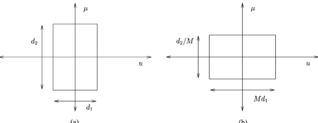
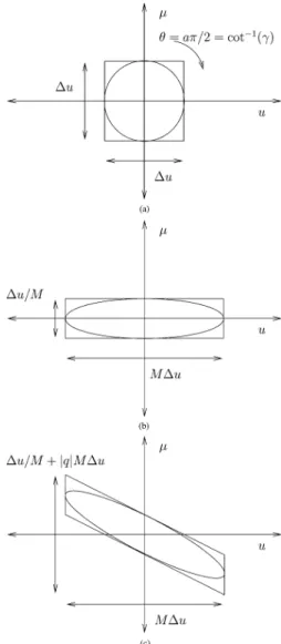
Fig. 1. Effect of scaling on the Wigner distribution. (a) Before scaling operation. (b) After scaling operation with parameter M.

Fig. 2. Effect of Fourier transformation on the Wigner distribution. (a) Before Fourier transformation. (b) After Fourier transformation.

For a signal with rectangular time-frequency support, the time-bandwidth product is equal to the number of degrees of freedom. This is not true for signals with other support shapes. While we have observed that LCTs do not change the number of degrees of freedom of a signal, they may change its time– bandwidth product. This will be illustrated in what follows.

C. Effects of Special LCTs on the Wigner Distribution

Here we discuss the effects of certain operations, all special cases of LCTs, on the Wigner distribution of a signal. These are of interest since we will decompose general LCTs in terms of these operations.

1) Scaling: The scaling operation is a special case of the LCT

defined as

(5) (6) Its effect on the WD is given by

(7) where . The scaling operation does not change the sup-port area, time-bandwidth product, or required number of sam-ples (Fig. 1), but it changes the sampling intervals in both the time and frequency domains by factors of and respectively.

2) Fourier Transformation: The ordinary Fourier transform

operation is also a special case of the LCT

(8)

(9) The subscript “ ” reminds us that the definition of the Fourier transform as a special case of LCTs differs from the conven-tional definition by the factor . Readers wishing to under-stand the technical reason behind this inconsequential discrep-ancy may consult [1], [2]. The effect of Fourier transformation on the WD is given by

(10) which is a rotation of in the clockwise direction (Fig. 2), which again does not change the time–bandwidth product.

3) Chirp Multiplication: The chirp multiplication (CM)

op-eration is another special case of the LCT

(11) (12) Its effect on the WD is

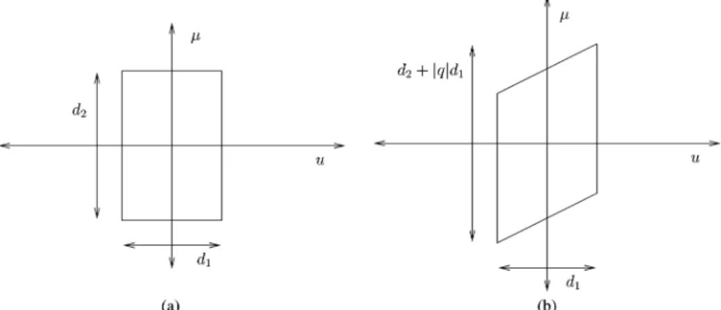
(13) Although the support area and therefore the number of de-grees of freedom are preserved after chirp multiplication, the time–bandwidth product increases. This is due to the increase in signal bandwidth as a result of vertical shearing of the WD

(Fig. 3). The new time–bandwidth product is .

If we wish a signal with such a support to be recoverable from its samples in the conventional manner, this is the number of

Fig. 3. Effect of chirp multiplication on the Wigner distribution. (a) Before chirp multiplication. (b) After chirp multiplication.

Fig. 4. Effect of fractional Fourier transformation on the Wigner distribution. (a) Before FRT operation. (b) After FRT operation.

samples we need. (The sampling interval in the time domain is and that in the frequency domain is .) The chirp convolution (CC) operation is the dual of the chirp multiplication and corresponds to a horizontal, rather than a ver-tical shear in the time-frequency plane:

(14) (15) Its effect on the WD is

(16)

4) Fractional Fourier Transformation: The th-order

frac-tional Fourier transform (FRT) [2], [38]–[44] of a function , denoted , is most commonly defined as

(17)

when and when and

when , where is an integer.

The square root is defined such that the argument of the result

lies in the interval . For ,

can be rewritten without ambiguity as

(18) where is the sign function. When is outside the interval , we need simply replace by its modulo 4 equiva-lent lying in this interval and use this value in (18).

The FRT is also a special case of the LCT with matrix

(19) differing only by the factor :

(20) Again the subscript “ ” denotes this inconsequential discrep-ancy between the definition of the FRT given by (17) and the FRT defined as a special case of the LCT [1], [2]. The FRT ro-tates the WD in the clockwise direction with an angle of

, as shown in Fig. 4:

III. SYSTEMATICANALYSIS OFDECOMPOSITIONS AND METHODI

The proposed algorithms use matrix factorizations to decom-pose LCTs into cascade combinations of the elementary LCT blocks discussed above. Since each stage can be computed in time, the overall LCT can also be. Numerous such de-compositions are possible [2], but they are not equally suited for numerical purposes. For instance, direct naive application of the decomposition of chirp multiplication, Fourier transformation, scaling (magnification), and again chirp multiplication, which suggests itself upon inspection of (1) will in general lead to very high sampling rates. We have carried out a systematic exhaustive analysis of all possible decompositions of arbitrary LCTs into the three basic operations of scaling, chirp multiplication (CM), and Fourier transformation (FT). We have considered all possible decompositions with three, four, and five cascade blocks. Every permutation has been checked to see if that decomposition is capable of expressing an LCT with arbitrary parameters.

It is well known that arbitrary LCTs can be decomposed in

either the form or , where and

are the chirp multiplication and convolution operations respec-tively [2]. Chirp convolutions can be realized as a Fourier trans-form followed by a chirp multiplication followed by an inverse Fourier transform (the Fourier transform of a chirp is also a chirp). Since we already consider all permutations involving chirp multiplication and Fourier transformation, approaches in-volving chirp convolution are also included in our development. While generating all possible decompositions through per-mutations, duplicate decompositions arise. For example, two

consecutive scaling or two consecutive chirp multiplication op-erations can both be collapsed into one. Or, for instance, in the case of five-stage decompositions with more free parameters than the three free parameters of LCTs, we have the freedom of choosing the additional parameters. When we select the scaling parameter as 1, this reduces to an equivalent four stage decom-position. In other words, some decompositions turn out to be equivalent to others, reducing the total number of possible de-compositions.

Careful consideration shows that there are a total of 16 dis-tinct decompositions. Four of these have four stages and 12 of them have five stages; decompositions with three stages are not flexible enough to match arbitrary LCTs. However, some de-compositions among this 16 are equivalent in implementation. For example a scaling and FT cascade can be replaced with a FT and inverse scaling cascade, a trivial and inconsequential differ-ence. When such trivial replacements are deducted from the set of 16 decompositions, we end up with 12 decompositions. We will immediately eliminate two of these decompositions. These two decompositions involve significantly more computational load than the others. As will be seen, the CM stages, especially when they occur early in the cascade, require us to increase the sampling rate and thus the complexity. Generally speaking it is desirable to have as few CM stages as possible and to have them appear as late in the cascade as possible. Therefore, we eliminate the two decompositions having three CM stages. Fi-nally, our exhaustive consideration and careful sorting out of all decompositions with three, four, and five stages leaves us with ten distinct decompositions to consider: see equations (22)–(31) shown at the bottom of the page. Recall that the diagonal

ma-(22) (23) (24) (25) (26) (27) (28) (29) (30) (31)

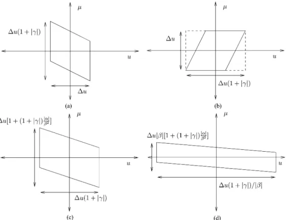
Fig. 5. Sequence of geometrical distortions for the decomposition in (22). The parallelogram in (c) is obtained by shearing the dashed rectangle in (b) in order to cover the worst case. (a) After the first stage: CM I. (b) After the second stage: FT. (c) After the third stage: CM II. (d) After the fourth stage: scaling.

trices correspond to scaling, the skew-diagonal ones to FT, and the lower-triangular ones to CM. The parameters , , of these operations are chosen in terms of the elements , , , of the matrix so as to equate the left and right hands of the above equations [see (2)].

Scaling and FT do not require an increase in the number of samples. However, since CM will change the time-bandwidth product, we introduce 2 oversampling when confronted with the first CM operation, to allow us room to maneuver. We will however try to avoid oversampling beyond this, as much as pos-sible. Specifically, we will impose any necessary restrictions so as to avoid further oversampling until the stage that involves the very last CM.

We will make sure that after each stage, the number of sam-ples is sufficient (in the Nyquist sense) for recovery of the con-tinuous signal. In order to illustrate how we deal with each de-composition, we consider the decomposition given in (22) as an example (Fig. 5). For graphical purposes, here we assumed that the initial time-frequency support is a square of edge length rather than a circle. Since we require that samples be suffi-cient, we must ensure that the time–bandwidth product does not

exceed :

(32) Therefore, we obtain the restriction for the pa-rameter appearing in the first chirp multiplication operation. This restriction ensures that oversampling by two is sufficient,

by ensuring that the bandwidth following the geometric distor-tion has not increased by more than a factor of two. After the FT, the second chirp multiplication operation, and the scaling operation, the time-bandwidth product becomes

(33)

Note that the parallelogram in Fig. 5(c) is obtained by shearing the dashed rectangle in Fig. 5(b) in order to cover the worst case. Is the above expression greater than and if so, how greater is it? Let denote the additional oversampling factor required. Equating the above expression to the number of samples corresponding to a total of oversampling, leads us to the minimum value of as

(34)

If the right-hand side of this expression turns out to be , that means that we do not need any additional oversampling, in which case we simply take . Before continuing, we also note that the scaling operation merely changes the sampling interval in the sense of reinterpretation of the same samples with a scaled sampling interval, in a manner which corresponds to scaling of the underlying continuous signal.

Thus, by carefully following the evolution of the time-fre-quency support region through each stage of the decomposition, we have obtained i) any necessary restrictions on the parameters

TABLE I

RESTRICTIONS ANDOVERSAMPLINGFACTORS

TABLE II

COMPUTATIONALCOMPLEXITIES.I(x; y) STANDS FOR THECOST TOINTERPOLATEx SAMPLES BY AFACTOR OFyTOOBTAIN

xy SAMPLES ANDS(z) STANDS FOR THECOST OF THESCALINGOPERATION ONz SAMPLES

of the stages appearing in the decomposition, so that oversam-pling beyond 2 is not required until the last CM stage, ii) the additional oversampling factor which may be needed before the last CM stage to fully represent the continuous output signal. We underline that these considerations are guided by our goal to accommodate arbitrary input signals. In those cases where there exists some a priori knowledge of the input signal or the signal is restricted to a particular class, it may be possible to customize the approach here with benefit.

The same procedure has been repeated for the decomposi-tions given in (23)–(31), and the results are given in Table I. It will be convenient to choose as the smallest integer sat-isfying the applicable inequality.

We have also added together the computational complexity of each stage to obtain the overall computational complexity of each decomposition and presented these in Table II. These com-plexity expressions will be reconsidered with a specific expres-sion for in Section V.

Observation of Table I reveals a natural grouping of the ten decompositions. The decompositions given in (22)–(24) exhibit the same restriction and oversampling factors. Likewise, the de-compositions given in (25)–(27) share the same restriction and oversampling factors. Moreover, the restrictions of these two groups are complementary, the first three can be used for and the last three can be used for , spanning the whole parameter space of LCTs.

TABLE III

PERCENTAGEERRORS FORDIFFERENTFUNCTIONSF , TRANSFORMST ,AND

ALGORITHMSA

Finally, we observe that the computational complexity of the third and last group of four decompositions is larger than the others. This group has a term with complexity

due to the second CM operation being followed by a DFT op-eration. Therefore, we discard the last four decompositions be-longing to the third group. It should be noted that our elimination procedure is primarily based on complexity as opposed to error. However, as we will see in Table III, the algorithm obtained pro-duces results with errors as small as can be reasonably expected; therefore we have not really lost anything by basing our proce-dure primarily on complexity.

Use of the information summarized in the two tables finally leads us to choose to work with two decompositions, one from the first and one from the second group of three. To ensure that oversampling by two is sufficient, we ended up using two com-plementary decompositions for different regions of the param-eter space. Since they have a slightly lower complexity, we will prefer to work with the second decomposition in both groups, whose advantage arises primarily from the relative positions of the scaling and CM operations. The algorithm can now be out-lined as follows.

• If , use the decomposition

(35) In operator notation

(36) where represents the oversampling operation. The minimum value of is

(37) • If , use the decomposition

(38) In operator notation

(39) The minimum value of is:

(40) A recent work also discusses the use of decompositions to an-alyze algorithms for related transforms [45]. This work also

em-phasizes the importance of tracking the time-bandwidth product through successive stages of the decomposition and sets forth a systematic, uniform, and general approach to determining the overall increase in time–bandwidth product of the final trans-formed signal. We have chosen to avoid unnecessary increases in the time-bandwidth product in the early stages to avoid in-creasing the number of samples until the last CM stage, where the major and unavoidable increase in sampling rate occurs.

IV. METHODII

The second approach we discuss is based on the fol-lowing decomposition involving the FRT, scaling, and chirp multiplication:

(41) Here , where is the order of the FRT, is the chirp multiplication parameter, and is the scaling factor. As we will see, these three parameters are sufficient to satisfy the above equality for arbitrary ABCD matrices, so that this decomposi-tion is capable of representing arbitrary LCTs. Since the fast method proposed in [11] can be used for the computation of the FRT, this decomposition leads to a fast algorithm for LCTs. This decomposition was inspired by the optical interpretation in [44] and is also a special case of the widely known Iwasawa decomposition [46]–[48]. It was also proposed later in [35] and [45]. Fig. 6 illustrates the sequence of geometrical distortions corresponding to this decomposition, where the initial time-fre-quency support is a circle of diameter .

If we multiply out the right-hand side of (41) and replace the matrix entries , , , with , , , we obtain

(42) which is equivalent to four equations which we can solve for ,

, :

(43)

(44)

(45) The ranges of the square root and the arccotangent both lie in . Fig. 6 shows the geometric effect of the decompo-sition stages on the WD of a function, which is rotation, scaling, and shearing, respectively. In operator notation this algorithm can be expressed as

(46) In this method, the first operation is a FRT, whose fast compu-tation in time is presented in [11] and [49]. (Other works dealing with fast computation of the FRT include [50]

Fig. 6. Sequence of geometrical distortions for the decomposition in (41). (a) After the first stage: FRT. (b) After the second stage: scaling. (c) After the third stage: CM.

and [51].) The algorithm presented in [11] was based on decom-posing the FRT into a CM followed by a CC followed by a final CM, and computed the samples of the continuous FRT in terms of the samples of the original signal. Just as in the present work, care was taken to ensure that the output samples represented the continuous FRT in the Nyquist–Shannon sense. The presently discussed algorithm employs the algorithm in [11] as a subrou-tine. The only approximation in this subroutine comes from the step involving chirp convolution in which a DFT/FFT is used to approximate the samples of the continuous FT. No other ap-proximation need be made, either in this subroutine or in any of the other operations that we employ. Thus, the only source of approximation can be traced to the evaluation of a continuous FT by use of a DFT (implemented with a FFT), which is a con-sequence of the fundamental fact that the signal energy cannot be confined to finite intervals in both domains. The second op-eration in this method is scaling, which only involves a reinter-pretation of the same samples with a scaled sampling interval. The final operation is CM which takes time, leading to an overall complexity of . (Detailed expressions will be given in Section V.) As in the first method, it is again necessary

to ensure that the output samples are sufficient to represent the transformed signal in the Nyquist–Shannon sense. Since LCTs distort the original time-frequency support, both the time and frequency extent of the signal, as well as its time–bandwidth product may increase, despite the fact that the area of the support remains the same. Therefore, a greater number of samples than may be needed to represent the transformed signal (unless we use some sophisticated basis to represent the signals) [35].

Delaying confrontation with the necessity to deal with this greater number of samples until the very last step is a signifi-cant advantage of this method. Since the FRT corresponds to ro-tation and scaling only to reinterprero-tation of the samples, these steps do not require us to increase the number of samples. At the last CM step, if we multiply the samples of the intermediate result with the samples of the chirp, the samples obtained will be good approximations of the true samples of the transformed signal at that sampling interval. If these samples are sufficient for our purposes, nothing further need be done. However, in gen-eral these samples will be below the Nyquist rate for the trans-formed signal and will not be sufficient for full recovery of the continuous function. To obtain a sufficient number of samples that will allow full recovery, we must interpolate the interme-diate result at least by a factor corresponding to the increase in time–bandwidth product

(47) Again, for convenience we choose to be the smallest integer satisfying this inequality.

V. NUMERICALRESULTS ANDCOMPARISON OFMETHODS We have considered several examples to illustrate and com-pare the presented methods. We refer to the first algorithm in-volving Fourier transformation, scaling, and chirp multiplica-tion as A1, and the second algorithm involving the fracmultiplica-tional Fourier transform as A2. We consider the chirped pulse

func-tion , denoted F1, and the trapezoidal

func-tion , denoted F2

. Since these two functions are well confined to a circle with diameter we take . We also consider the bi-nary sequence 01101010 occupying with each bit 2 units in length, so that . This binary sequence is denoted by F3 and the function shown in Fig. 7 is denoted by F4, again with . These choices for result in 0 , 0.0002%, 0.47%, 0.03% of the energies of F1, F2, F3, F4 respectively, to fall outside the chosen frequency extents. The chosen time ex-tents include all of the energies of F2, F3, F4 and virtually all of the energy of F1. We consider two transforms, the first (T1)

with parameters , and the second (T2)

with parameters . The LCTs T1 and T2 of the func-tions F1, F2, F3, F4 have been computed both by the presented fast methods A1 and A2 and by a highly inefficient brute force numerical approach which is here taken as a reference.

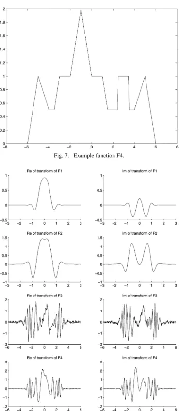
The results for all functions (F1, F2, F3, F4) and both algo-rithms (A1, A2) are plotted in Fig. 8 for transform T1, and tab-ulated in Table III for both transforms (T1, T2). Also shown are the errors that arise when using the DFT in approximating the FT of the same functions, which serves as a reference. (The error

Fig. 7. Example function F4.

Fig. 8. Transforms (T1) of F1, F2, F3, F4. The results obtained with Methods I and II and the reference result have been plotted with dotted, dashed, and solid lines respectively. However, in most cases these lines are indistinguishable since the results are very close.

is defined as the energy of the difference normalized by the en-ergy of the reference, expressed as a percentage.)

The key observations that can be made from this table are as follows. The errors obtained depend on the function, since dif-ferent functions have difdif-ferent amounts of energy contained in their tails which fall outside the assumed time and frequency

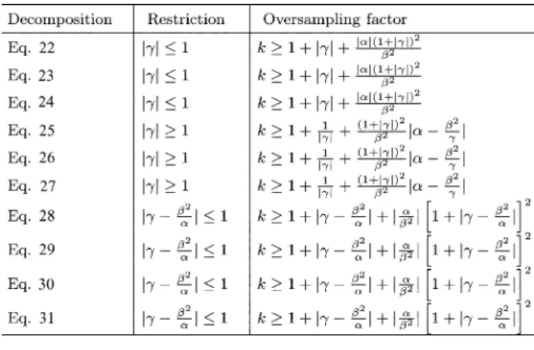
Fig. 9. Percentage errors versusN for selected functions and transforms [35].

extents (or assumed time-frequency region). For those cases in which the error is large, such as F3, this means that we have de-termined the time–bandwidth product less conservatively than the other examples, and the error can be reduced by increasing . Generally speaking, the errors obtained depend very little on the transform parameters or which method we use, and are com-parable to the error arising when we use the DFT to approximate the FT. Since a DFT lies at the heart of both methods, this is the smallest error we could have hoped to achieve to begin with.

Fig. 9 shows the error versus number of sample points for selected functions and transforms. We observe that the error de-creases steeply at first with increasing as expected, but satu-rates when we approach and exceed the time-bandwidth product of the signals (here 64). This demonstrates that the number of samples can be chosen comparable to the time–bandwidth product, which is the smallest number we can expect to work with, and need not be chosen larger. A2 was used to obtain this plot for illustration purposes but similar results can also be ob-tained when we use A1.

We now turn our attention to discussing the complexity (cost) of the algorithms as a function of , the number of sample points. Based on the preceding paragraph, can be chosen comparable to the time-bandwidth product so that the expres-sions given below can also be interpreted as functions of time-bandwidth product.

The computational complexity of the first method is given by either of the following expressions, depending on which decom-position is used (which was determined by whether or not, respectively):

• ;

•

.

On the other hand, for the second method, one of the fol-lowing applies depending on the branch of the FRT algorithm

used, which depends on whether or ,

respectively. Not surprisingly, this turns out to be the same as

the condition or , respectively:

• ;

•

.

The above expressions are derived by calculating the com-plexity of the FRT algorithm of [11] in its most efficient

im-plementation , and

adding the cost of the other operations.

Although included for completeness, the cost of the scaling operation is minimal and not of much consequence, since it amounts only to a reinterpretation of samples. In the above expressions, stands for the cost to interpolate samples by a factor of to obtain samples. There are several efficient approximate interpolation methods which have complexities of order [52]. We will write this cost as where is a constant.

Taking the difference of the costs of the two methods, Method II will have lower cost if

(48) where and are associated with Method I and Method II respectively. If we go back to the steps of each method, we ob-serve that it is usually possible to choose much more tightly than . Numerical simulations also confirm that is usually smaller than . Therefore, either method may turn out to have lower cost depending on the values of , , , and it is not possible in general to declare one method superior over the other in this respect. If need be, both methods can be incorporated in the same code and the more efficient one invoked based on the parameters, but in many cases the difference may not be very significant. However, apart from its effect on cost of computa-tion, having the lowest oversampling factor is desirable in itself since it produces an output represented with the least number of samples. This is a plus for Method II, which we also favor for its elegant construction.

Finally, we compare Method I and Method II, with the direct use of the well-known CM-CC-CM decomposition [2] without the kind of sampling rate management undertaken in this paper (“Method III”):

(49) which is valid as long as . The CC stage has been imple-mented in the Fourier domain as a CM operation. At each step of the process, the sampling rate has been chosen as the min-imum compatible with the shear-induced increases in the time and frequency extents. Considering T1, the minimum oversam-pling rate is , , for Methods I, II, and III, respectively. With the more demanding T2, the minimum value of is , , , respectively. Larger values of and thus larger total numbers of samples not only result in representational redundancy, but also they translate into greater computational time. For instance, for F4 and T2, the time of computation in seconds is , , for Methods I, II, and III, respectively (obtained with MATLAB running on a personal computer), demonstrating that Method III is significantly slower. The corresponding per-centage errors are comparable as expected: , , , respectively.

VI. CONCLUSION

In this paper, two algorithms for the computation of linear canonical transforms (LCTs) from the samples of the input signal in time are discussed. Our approach is based on concepts from signal analysis and processing rather than conventional numerical analysis. With careful consideration of sampling issues, can be chosen very close to the time-band-width product of the signals, and need not be much larger. The transform output may have a higher time-bandwidth product due to the nature of the transform family.

Both algorithms relate the samples of the input function to the samples of the continuous LCT of this function in the same sense that the fast Fourier transform (FFT) implementation of the dis-crete Fourier transform (DFT) computes the samples of the con-tinuous FT of a function. Since the sampling rates are carefully controlled, the output samples obtained are accurate approxima-tions to the true ones and the continuous LCT can be recovered via interpolation of these samples. The only inevitable source of deviation from exactness arises from the fundamental fact that a signal and its transform cannot both be of finite extent. This is the same source of deviation encountered when using the DFT/FFT to compute the continuous FT. Thus, the algorithms compute LCTs with a performance similar to the DFT/FFT in computing the Fourier transform, both in terms of speed and accuracy.

The fact that the two methods, although being arrived at from considerably different starting points, both exhibit similar limits in performance, strongly suggests that the performance achieved is close to the best achievable. Indeed, as already noted, it is difficult to expect an accuracy which is better than that of the DFT in approximating the FT, and a cost which is

less than with being close to the

time–band-width product. Despite the different decompositions employed, an interesting structural similarity emerges between the two methods in their optimized forms. Both methods have two branches, the first one determined by whether or not, and the second one determined by whether or not. If is expressed in terms of the LCT parameters , , , we see that the two conditions are the same. Therefore, the separation of the LCT parameter space into two regions is most likely not a characteristic of the algorithm chosen, but an intrinsic structural property of the LCT parameter space.

Compared to earlier approaches, these algorithms not only handle a much more general family of integrals, but also effec-tively address certain difficulties, limitations, or tradeoffs that arise in other approaches to computing the Fresnel integral, which is of importance in the theory of diffraction (see [45] for a systematic comparison of several approaches). These algorithms can also be used for efficient realization of filtering in linear canonical transform domains [53].

ACKNOWLEDGMENT

The authors would like to thank O. Arikan of the Electrical Engineering and L. Barker of the Mathematics Departments of Bilkent University, Ankara, Turkey, for helpful discussions. A. Koç would like to thank L. Hesselink of the Electrical Engineering Department of Stanford University, Stanford, CA, for his support. H. M. Ozaktas acknowledges partial support of the Turkish Academy of Sciences and partial support of

the Scientific and Technological Research Council of Turkey (TUBITAK) under grant number EEEAG-105E065.

REFERENCES

[1] K. B. Wolf, Integral Transforms in Science and Engineering. New York: Plenum, 1979, vol. Construction and Properties of Canonical Transforms, ch. 9.

[2] H. M. Ozaktas, Z. Zalevsky, and M. A. Kutay, The Fractional Fourier

Transform with Applications in Optics and Signal Processing. New York: Wiley, 2001.

[3] M. J. Bastiaans, “Wigner distribution function and its application to first-order optics,” J. Opt. Soc. Amer., vol. 69, pp. 1710–1716, 1979. [4] M. J. Bastiaans, “Applications of the Wigner distribution function in

optics,” in The Wigner Distribution: Theory and Applications in Signal

Processing, Amsterdam, The Netherlands, 1997, pp. 375–426.

[5] S. Abe and J. T. Sheridan, “Generalization of the fractional Fourier transformation to an arbitrary linear lossless transformation: An oper-ator approach,” J. Phys. A, vol. 27, pp. 4179–4187, 1994.

[6] S. Abe and J. T. Sheridan, “Optical operations on wavefunctions as the Abelian subgroups of the special affine Fourier transformation,” Optics

Letters, vol. 19, pp. 1801–1803, 1994.

[7] A. E. Siegman, Lasers. Mill Valley, CA: University Science Books, 1986.

[8] D. F. V. James and G. S. Agarwal, “The generalized Fresnel transform and its applications to optics,” Opt. Commun., vol. 126, pp. 207–212, 1996.

[9] C. Palma and V. Bagini, “Extension of the Fresnel transform to ABCD systems,” J. Opt. Soc. Amer. A, vol. 14, pp. 1774–1779, 1997. [10] J. Hua, L. Liu, and G. Li, “Extended fractional Fourier transforms,” J.

Opt. Soc. Amer. A, vol. 14, pp. 3316–3322, 1997.

[11] H. M. Ozaktas, O. Arikan, M. A. Kutay, and G. Bozda˘gi, “Digital computation of the fractional Fourier transform,” IEEE Trans. Signal

Process., vol. 44, no. 9, pp. 2141–2150, Sep. 1996.

[12] B. M. Hennelly and J. T. Sheridan, “Fast numerical algorithm for the linear canonical transform,” J Opt. Soc. Amer. A, vol. 22, pp. 928–937, 2005.

[13] N. M. Atakishiyev and K. B. Wolf, “Fractional Fourier-Kravchuk trans-form,” J. Opt. Soc. Amer. A, vol. 14, pp. 1467–1477, 1997.

[14] S.-C. Pei and M.-H. Yeh, “Improved discrete fractional Fourier trans-form,” Opt. Lett., vol. 22, pp. 1047–1049, 1997.

[15] N. M. Atakishiyev, S. M. Chumakov, and K. B. Wolf, “Wigner distribu-tion funcdistribu-tion for finite systems,” J. Math. Phys., vol. 39, pp. 6247–6261, 1998.

[16] N. M. Atakishiyev, L. E. Vicent, and K. B. Wolf, “Continuous versus discrete fractional Fourier transforms,” J. Comput. Appl. Math., vol. 107, pp. 73–95, 1999.

[17] S. C. Pei, M. H. Yeh, and C. C. Tseng, “Discrete fractional Fourier transform based on orthogonal projections,” IEEE Trans. Signal

Process., vol. 47, no. 5, pp. 1335–1348, May 1999.

[18] S.-C. Pei, M.-H. Yeh, and T.-L. Luo, “Fractional Fourier series expan-sion for finite signals and dual extenexpan-sion to discrete-time fractional Fourier transform,” IEEE Trans. Signal Process., vol. 47, no. 10, pp. 2883–2888, Oct. 1999.

[19] T. Erseghe, P. Kraniauskas, and G. Cariolaro, “Unified fractional Fourier transform and sampling theorem,” IEEE Trans. Signal

Process., vol. 47, no. 12, pp. 3419–3423, Dec. 1999.

[20] M. A. Kutay, H. Özaktas¸, H. M. Ozaktas, and O. Arikan, “The frac-tional Fourier domain decomposition,” Signal Process., vol. 77, pp. 105–109, 1999.

[21] A. I. Zayed and A. G. Garcia, “New sampling formulae for the frac-tional Fourier transform,” Signal Process., vol. 77, pp. 111–114, 1999. [22] C. Candan, M. A. Kutay, and H. M. Ozaktas, “The discrete fractional Fourier transform,” IEEE Trans. Signal Process., vol. 48, no. 5, pp. 1329–1337, May 2000.

[23] I. S¸. Yetik, M. A. Kutay, H.Özaktas¸, and H. M. Ozaktas, “Continuous and discrete fractional Fourier domain decomposition,” in Proc. IEEE

Int. Conf. Acoustics, Speech, Signal Processing, 2000, pp. I:93–96.

[24] S. C. Pei and M. H. Yeh, “The discrete fractional cosine and sine trans-forms,” IEEE Trans. Signal Process., vol. 49, no. 6, pp. 1198–1207, Jun. 2001.

[25] G. Cariolaro, T. Erseghe, and P. Kraniauskas, “The fractional discrete cosine transform,” IEEE Transactions Signal Process., vol. 50, no. 4, pp. 902–911, Apr. 2002.

[26] L. Barker, “Continuum quantum systems as limits of discrete quantum systems. IV. Affine canonical transforms,” J. Math. Phys., vol. 44, pp. 1535–1553, 2003.

[27] C. Candan and H. M. Ozaktas, “Sampling and series expansion theo-rems for fractional Fourier and other transforms,” Signal Process., vol. 83, pp. 1455–1457, 2003.

[28] J. G. Vargas-Rubio and B. Santhanam, “On the multiangle centered discrete fractional Fourier transform,” IEEE Signal Process. Lett., vol. 12, no. 4, pp. 273–276, 2005.

[29] M. H. Yeh, “Angular decompositions for the discrete fractional signal transforms,” Signal Process., vol. 85, pp. 537–547, 2005.

[30] K. B. Wolf, “Finite systems, fractional Fourier transforms and their finite phase spaces,” Czech. J. Phys., vol. 55, pp. 1527–1534, 2005. [31] K. B. Wolf, “Finite systems on phase space,” Int. J. Mod. Phys. B, vol.

20, pt. 2 Sp. Iss, pp. 1956–1967, 2006.

[32] K. B. Wolf and G. Krotzsch, “Geometry and dynamics in the fractional discrete Fourier transform,” J. Opt. Soc. Amer. A, vol. 24, pp. 651–658, 2007.

[33] D. Mendlovic, Z. Zalevsky, and N. Konforti, “Computation consider-ations and fast algorithms for calculating the diffraction integral,” J.

Mod. Opt., vol. 44, pp. 407–414, 1997.

[34] D. Mas, J. Garcia, C. Ferreira, L. M. Bernardo, and F. Marinho, “Fast algorithms for free-space diffraction patterns calculation,” Opt.

Commun., vol. 164, pp. 233–245, 1999.

[35] H. M. Ozaktas, A. Koç, I. Sari, and M. A. Kutay, “Efficient computation of quadratic-phase integrals in optics,” Opt. Lett., vol. 31, pp. 35–37, 2006.

[36] F. Hlawatsch and G. F. Boudreaux-Bartels, “Linear and quadratic time-frequency signal representations,” IEEE Signal Process. Mag., vol. 9, no. 2, pp. 21–67, Apr. 1992.

[37] L. Cohen, Time-Frequency Analysis. Englewood Cliffs, NJ: Prentice-Hall, 1995.

[38] D. Mendlovic and H. M. Ozaktas, “Fractional Fourier transforms and their optical implementation: I,” J. Opt. Soc. Amer. A, vol. 10, pp. 1875–1881, 1993.

[39] H. M. Ozaktas and D. Mendlovic, “Fractional Fourier transforms and their optical implementation: II,” J. Opt. Soc. Amer. A, vol. 10, pp. 2522–2531, 1993.

[40] H. M. Ozaktas and D. Mendlovic, “Fourier transforms of fractional order and their optical interpretation,” Opt. Commun., vol. 101, pp. 163–169, 1993.

[41] H. M. Ozaktas, B. Barshan, D. Mendlovic, and L. Onural, “Convolu-tion, filtering, and multiplexing in fractional Fourier domains and their relation to chirp and wavelet transforms,” J. Opt. Soc. Amer. A, vol. 11, pp. 547–559, 1994.

[42] L. B. Almeida, “The fractional Fourier transform and time-frequency representations,” IEEE Trans. Signal Process., vol. 42, no. 11, pp. 3084–3091, Nov. 1994.

[43] H. M. Ozaktas and D. Mendlovic, “Fractional Fourier optics,” J. Opt.

Soc. Amer. A, vol. 12, pp. 743–751, 1995.

[44] H. M. Ozaktas and M. F. Erden, “Relationships among ray optical, Gaussian beam, and fractional Fourier transform descriptions of first-order optical systems,” Opt. Commun., vol. 143, pp. 75–86, 1997.

[45] B. M. Hennelly and J. T. Sheridan, “Generalizing, optimizing, and inventing numerical algorithms for the fractional Fourier, Fresnel, and linear canonical transforms,” J. Opt. Soc. America. A, vol. 22, pp. 917–927, 2005.

[46] T. Alieva and M. J. Bastiaans, “Alternative representation of the linear canonical integral transform,” Opt. Lett., vol. 30, pp. 3302–3304, 2005.

[47] M. J. Bastiaans and T. Alieva, “Synthesis of an arbitrary ABCD system with fixed lens positions,” Opt. Lett., vol. 31, pp. 2414–2416, 2006. [48] J. A. Rodrigo, T. Alieva, and M. L. Calvo, “Optical system design for

orthosymplectic transformations in phase space,” J. Opt. Soc. Amer. A, vol. 23, pp. 2494–2500, 2006.

[49] X. Yang, Q. Tan, X. Wei, Y. Xiang, Y. Yan, and G. Jin, “Improved fast fractional-Fourier-transform algorithm,” J. Opt. Soc. Amer. A, vol. 21, pp. 1677–1681, 2004.

[50] J. Garcia, D. Mas, and R. G. Dorsch, “Fractional Fourier transform calculation through the fast Fourier transform algorithm,” Appl. Opt., vol. 35, pp. 7013–7018, 1996.

[51] F. J. Marinho and L. M. Bernardo, “Numerical calculation of fractional Fourier transforms with a single fast Fourier transform algorithm,” J.

Opt. Soc. Amer. A, vol. 15, pp. 2111–2116, 1998.

[52] D. B. Turek, “Design of efficient digital interpolation filters for integer upsampling,” M.E. thesis, MIT, Cambridge, MA, 2004.

[53] B. Barshan, M. A. Kutay, and H. M. Ozaktas, “Optimal filtering with linear canonical transformations,” Opt. Commun., vol. 135, pp. 32–36, 1997.

Aykut Koç was born in Eskisehir, Turkey, in 1982.

He received the B.S. degree in electrical and elec-tronics engineering from Bilkent University, Ankara, Turkey, in 2005 and the M.S. degree in electrical en-gineering from Stanford University, Stanford, CA, in 2007. He is currently working towards the Ph.D. de-gree under the supervision of Prof. L. Hesselink at the Solid State and Photonics Laboratory, Electrical Engineering Department, Stanford University.

As an undergraduate at Bilkent University, he con-tributed to the development of efficient algorithms for computing families of integrals with applications in diffraction and optical signal processing. His academic interests include Fourier optics, signal pro-cessing, the fractional Fourier transform and its applications, and nanooptics and nanostructured metallic surfaces, particularly plasmonic resonance effects.

Haldun M. Ozaktas (M’07) received the B.S.

de-gree from Middle East Technical University, Ankara, Turkey, in 1987 and the Ph.D. degree from Stanford University, Stanford, CA, in 1991.

He joined Bilkent University, Ankara, Turkey, in 1991, where he is presently a Professor of electrical engineering. In 1992, he was at the University of Erlangen-Nurnberg, Bavaria as an Alexander von Humboldt Foundation Postdoctoral Fellow. During summer 1994, he worked as a Consultant at Bell Laboratories, Holmdel, NJ. He is the author of ap-proximately 90 refereed journal articles, over 10 book chapters, and about 100 conference presentations and papers, over 35 of which have been invited. He is also author of the book The Fractional Fourier Transform (Wiley, 2001) and edited the book Three-Dimensional Television (Springer, 2008). His academic interests include signal and image processing, optical information processing, and optoelectronic and optically interconnected computing systems.

Dr. Ozaktas has a total of over 2500 citations to his work recorded in the Science Citation Index (ISI). He is the recipient of the 1998 ICO International Prize in Optics and one of the youngest recipients ever of the Scientific and Tech-nical Research Council of Turkey (TUBITAK) Science Award (1999), among other awards and prizes. He is also one of the youngest members of the Turkish Academy of Sciences and a Fellow of the Optical Society of America (OSA).

Cagatay Candan received the B.S. degree from

Middle East Technical University, Ankara, Turkey, in 1996, the M.S. degree from Bilkent University, Ankara, Turkey, in 1998, and the Ph.D. degree from the Georgia Institute of Technology, Atlanta in 2004. He is working in Middle East Technical Uni-versity as an Assistant Professor. His research interests are applications of fractional Fourier transform to time-frequency distributions, detection and estimation theory, statistical signal processing, and applications of statistical signal processing in communication systems and MIMO systems.

M. Alper Kutay was born in Konya, Turkey, in 1972.

He received the B.S., M.S., and Ph.D. degrees, all in electrical and electronics engineering, from Bilkent University, Ankara, Turkey, in 1993, 1995, and 1999, respectively.

During his graduate studies, he was a teaching and research assistant. From March 1999 to June 2000, he was with the Communications and Signal Processing Laboratory at Drexel University, Philadelphia, PA. He is now a Senior Research Scientist at the Scientific and Technical Research Council of Turkey-National Research Institute of Electronics and Cryptology (TUBITAK-UEKAE). He is the coauthor of the book The Fractional Fourier

Transform with Applications in Optics and Signal Processing (Wiley, 2001).

His current research areas include time-frequency signal representations, fractional Fourier transform, time-varying filtering, signal detection, signal enhancement, and radar signal processing.

Dr. Kutay was awarded third place in the 1994 IEEE Region 8 student paper contest for his work titled “An Adaptive Speckle Suppression Filter for Medical Ultrasonic Imaging.”