Computers in Biology and Medicine 116 (2020) 103547
Available online 20 November 2019
0010-4825/© 2019 Elsevier Ltd. All rights reserved.
Comparison of morphometric parameters in prediction of hydrocephalus
using random forests
Busra Ozgode Yigin
a,*, Oktay Algin
b,c,d, Gorkem Saygili
a,e aDepartment of Biomedical Engineering, Ankara University, Golbasi, Ankara, TurkeybDepartment of Radiology, City Hospital, Bilkent, Ankara, Turkey cDepartment of Radiology, Yildirim Beyazit University, Ankara, Turkey
dNational MR Research Center (UMRAM), City Hospital, Bilkent University, Ankara, Turkey
eDepartment of Interdisciplinary Neuroscience, Health Science Institute, Ankara University, Ankara, Turkey
A R T I C L E I N F O Keywords: Hydrocephalus Morphological parameters Feature importance Semi-automatic analysis A B S T R A C T
Ventricles of the human brain enlarge with aging, neurodegenerative diseases, intrinsic, and extrinsic pathol-ogies. The morphometric examination of neuroimages is an effective approach to assess structural changes occurring due to diseases such as hydrocephalus. In this study, we explored the effectiveness of commonly used morphological parameters in hydrocephalus diagnosis. For this purpose, the effect of six common morphometric parameters; Frontal Horns’ Length (FHL), Maximum Lateral Length (MLL), Biparietal Diameter (BPD), Evans’ Ratio (ER), Cella Media Ratio (CMR), and Frontal Horns’ Ratio (FHR) were compared in terms of their impor-tance in predicting hydrocephalus using a Random Forest classifier. The experimental results demonstrated that hydrocephalus can be detected with 91.46 % accuracy using all of these measurements. The accuracy of clas-sification using only CMR and FHL reached up to 93.33 %. In terms of individual performances, CMR and FHL were the top performers whereas BPD and FHR did not contribute as much to the overall accuracy.
1. Introduction
Brain ventricles are dilated with the accumulation of excessive ce-rebrospinal fluid which leads to a condition known as hydrocephalus. Hydrocephalus affects a wide range of people, from infants to elderly adults. Generally, the ventricular enlargement is measured using pa-rameters derived from the dimensions of the ventricles instead of their actual volumes. Different morphological parameters are used in the literature for the diagnosis of hydrocephalus such as Bicaudate Ratio (BCR), Bifrontal Index (BFI), Bioccipital Index (BOI), Biparietal Diam-eter (BPD), Cella Media Ratio (CMR), Evans’ Ratio (ER), Minimum Lateral Length (MLL), Third Ventricle Width (TVW), Third Ventricle Sylvian Fissure Ratio Index (TSFI), and Third Ventricle Ratio (TVR) [1,
2]. These parameters are useful not only for the diagnosis and classifi-cation of hydrocephalus but also for the follow-up and evaluation of the expansion of the ventricular system after operations such as ventricular shunts [3,4].
Diagnostic methods for hydrocephalus involve a mixture of clinical and imaging approaches. Accurate and effective evaluation of many CSF-related diseases, especially hydrocephalus, can be performed much
faster using new sequences and techniques developed in parallel with the progress in MRI technology. MRI is mostly preferred over CT since it may provide better detail of the borders of ventricles [5,6]. MRI is helpful in the diagnosis of hydrocephalus and helps in the management and postoperative follow-up of the patients [7,8].
In this paper, we aim to compare the performances of the above- mentioned parameters in hydrocephalus detection. For this purpose, we trained a random forest classifier to predict hydrocephalus and measure the importance of each parameter. To our knowledge, there is no other study in the literature that compares the performance of these parameters.
The rest of the paper is organized as follows: In section 2, we explain the methodology that we use to measure linear parameters and our classifier that we train on our dataset. Section 3 presents the experi-mental setup and results. We discuss our results in section 4. In section 5, we draw our conclusions and suggest possible topics for future research.
* Corresponding author.
E-mail addresses: [email protected] (B. Ozgode Yigin), [email protected] (O. Algin), [email protected] (G. Saygili).
Contents lists available at ScienceDirect
Computers in Biology and Medicine
journal homepage: http://www.elsevier.com/locate/compbiomed
https://doi.org/10.1016/j.compbiomed.2019.103547
2. Methodology
2.1. Measurements of linear parameters
All the measurements that are used in the calculation of parameters are demonstrated in Fig. 1. These measurements are:
a: MLL - The narrowest width between the lateral walls.
b: DSL - The internal diameter of the skull in the same line as MLL. c: MTD - Maximum transverse diameter of the skull.
d: BPD - Maximum width of internal diameter of the skull. e: DM - Inner diameter of the skull in the same line as FHL. f: FHL - Width of greatest span of frontal horns.
With these measurements the following parameters are calculated: - Evans’ Ratio (f
d): the ratio of maximum width of the frontal horns of
the lateral ventricles, f, and the greatest internal diameter of skull,
d [9]. ER was described by Evans [10] in 1942 as a method of
measurement of ventricular size in pediatric patients. Current guidelines state that an ER greater than 0.3 indicates hydrocephalus [5,11,12].
- Cella Media Ratio (a
c): the ratio of the minimum distance between
lateral walls of lateral ventricles in cella media region,a, and maximum transverse (external) diameter, c. It is expected to be smaller than 0.25 in normal cases [9].
- Frontal Horns’ Ratio (f
e): the ratio of maximum width of the frontal
horns of the lateral ventricles, f, and inner diameter of skull in the same line as f, e [9,13]. Mean FHR was found to be 0.302 by Singh et al. [14] similar as in the studies by Swati et al. [9] (0.30) and by Hahn et al. [15](0.31) on 200 normal CT scans.
CMR is expressed differently in different studies. We named these variations as CMR1, CMR2, and CMR3. Swati et al. [9] defined CMR as the ratio of the MLL (a) to MTD (c) with the threshold value of 0.25 for the diagnosis of hydrocephalus (CMR1). Kolsur et al. [16] defined CMR as the ratio of MLL (a) to BPD (d) (CMR2). Their threshold was 0.227. Patnaik et al. and Singh et al. [2,14] described CMR as the ratio of MLL (a) to DSL (b) with the threshold of 0.22 (CMR3). In another study, this threshold is selected as 0.295 [17]. Although measured differently, the same threshold values are used for these parameters in different studies. Therefore, it is confusing which threshold value to use for which parameter. Therefore, we calculated all these three variations of CMR and picked CMR1 as CMR because it provided the most accurate result.
2.2. Random forests for classification
Random Forest (RF) is one of the most popular machine learning algorithms because it provides accurate results without exhaustive hyper-parameter tuning and can be applied to both regression and classification problems. RF is an ensemble learner composed of decision trees. Decision trees are prone to over-fitting in contrast RF utilizes a bagging approach to cope with over-fitting. Additionally, RF requires no pre-processing of the feature space such as standardization and needs a fewer number of hyper-parameters to be set. Furthermore, RF uses its internal estimates and a small subset of features to measure feature importance. Considering all of these advantages, we preferred RF as our classifier [18–20]. The two most widely used feature importance mea-sures are impurity and permutation importance. For the impurity importance, a split that reduces impurity, hence the features used in the split are considered important. Based on this viewpoint, the impurity
Fig. 1. Illustration of the parameters for the evaluation of hydrocephalus; MLL (a), DSL (b), MTD (c), BPD (d), DM (e), FHL (f). Table 1
3 T MRI protocol used for the study. Sequences/
Parameters 3D- MPRAGE 3D-SPACE (with VFAM) T2W- TSE FLAIR TR/TE (ms) 2130=3:45 3000=579 6300=84 6000=405 TI (ms) 1100 – – 2100 Slice thickness 0.8 0.6 4 0.9 FOV*(mm) 230x230 240x240 220x220 230x230 Acquisition time (minute) 5 5 0.39 9 NEX 1 2 1 1 Number of slices 240 240 24 192 Flip angle (�) 8 100 180 –
Imaging plane Sagittal Sagittal Axial Sagittal
PAT factor 2 2 2 –
PAT mode GRAPPA GRAPPA GRAPPA – Voxel size (mm) 0.8x0.8x0.8 0.6x0.6x0.6 1x0.9x4 0.9x0.9x0.9
FA mode – T2 variant – –
Notes ¼ TI: time of inversion; 3D-SPACE: three-dimensional sampling perfec-tion with applicaperfec-tion-optimized contrasts using different flip angle evoluperfec-tions; 3D-MPRAGE: 3D T1W magnetization prepared rapid acquisition gradient-echo; T2W-TSE: T2 weighted turbo spin-echo; FLAIR: fluid-attenuated inversion-re-covery; NEX: number of excitations; FOV: field of view; PAT: parallel acquisition technique; GRAPPA: generalized auto calibrating partially parallel acquisitions.
Computers in Biology and Medicine 116 (2020) 103547
importance for a feature xi is computed by the sum over the number of
splits (across all tress) that include xi, proportionally to the number of
samples it splits [21,22]. Breiman [23] proposed to calculate the per-mutation importance by measuring the Mean Decrease Accuracy (MDA) of the forest when xi values are permuted randomly in the out-of-bag
samples [24]. Thanks to popular machine learning libraries [19,23,
25], both of these feature importance measures have shown their practical utility in an increasing number of experimental studies. Mea-sures based on the impurity reduction of splits, such as the Gini importance, are popular because they are simple and fast to compute. Scikit-learn library has a function to calculate the Gini, and we have used it to calculate the feature importance.
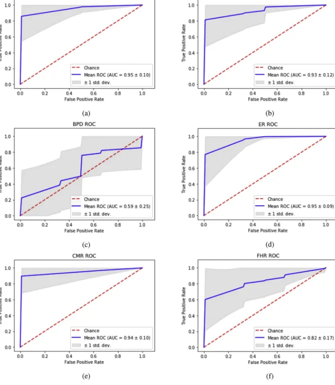
Fig. 2. ROC curves for the individual features as FHL, MLL, BPD, ER, CMR, and FHR respectively. AUC values are also shown on the graphs.
Table 2
The success of classification with the individual features.
Accuracy Recall AUC
Only FHL 95.0 % 0.95 0.94 �0:1 Only CMR 91.67 % 0.92 0.93�0:12 Only MLL 89.58 % 0.90 0.94�0:12 Only ER 86.25 % 0.86 0.95�0:09 Only FHR 75.42 % 0.75 0.83�0:16 Only BPD 57.7 % 0.58 0.58�0:24
Fig. 3. Left column shows ROC curves and right column shows feature-importance based random forest classifier. From top to bottom added features CMR, FHL, MLL, ER, FHR, and BPD, respectively.
Computers in Biology and Medicine 116 (2020) 103547
3. Experiments and results
3.1. Data and experimental setup
In our experiment we used MRI data from National Magnetic Reso-nance Research Center (UMRAM), Bilkent University. The study popu-lation composed of 48 subjects (21 males and 27 females) in the age group of 4–84 years, with 25 subjects diagnosed with hydrocephalus and 23 subjects diagnosed with normal. All images were taken by a trained and experienced neuroradiologist in standardized condition and manner. T2-weighted axial MR images in which all parameters were easily observed were preferred for the measurement of the parameters. One experienced neuroradiologists (O. A.) and one radiologist (S. E.) independently evaluated all MR images, blinded to clinical information. The subjects were labeled as hydrocephalus and healthy, based on morphological MR parameters and clinical findings, such as the pres-ence of headache, visual disturbances, vomiting, according to our pre-vious studies [7,26,27].
MRI examinations were performed using a 3T unit (Trio with Tim; Siemens Healthcare AG, Erlangen, Germany) with a birdcage- multichannel head coil. The 3-T MRI protocol is given in Table 1. The parameters were measured by two experienced neuroradiologists ac-cording to the literature [7,9–11,14]. Recent findings have shown that morphological measurements vary greatly depending on the slice loca-tion of the brain MR images [5,11]. Therefore, the parameters were defined and measured from the same locations of the patients based on registration with anterior and posterior commissure line.
The RF classification was implemented using Python programming language with Scikit-learn library. Since we have a limited number of data, we have applied 10-fold cross-validation to our data so that we could use the entire data set for both testing and training. It provides a good indication of the generalization error. K-fold cross-validation di-vides the data set into K subsets, and it uses the K-1 of the subsets for training and one for the test. The cross-validation procedure was repeated ten times, yielding ten random partitions of the original data. Receiver Operator Characteristic (ROC) curves, accuracy, recall, and the
area under the curve (AUC) values have been obtained by calculating the mean of ten times k-fold results.
3.2. Experimental results
The parameters mentioned in the previous sections will now be referred to as features. We applied our classifier with six features (FHL, BPD, MLL, ER, CMR, FHR) obtained from axial MR images. First, we aim to measure the success of each feature individually. Hence, we attained a confusion matrix for each feature. We used the ROC curve, AUC, accu-racy, and recall values as the performance criteria for RF classification. Accuracy, recall, AUC, and ROC results for 10-fold cross-validation for all individual features are represented in Fig. 2 and Table 2. The results
in Table 2 show that the FHL (95 %) and CMR (91.67 %) outperform
others in terms of accuracy. From the results, it is seen that especially FHL and CMR are leading in decision making, whereas FHR and BPD are the worst performers.
In our next experiment, we utilized all features together in our RF classifier and the order of importance of these features was obtained. These features were added to each other according to their effectiveness in decision-making. As can be seen from the accuracy scores in Fig. 3, the accuracy of our original model, which includes all six features, is 91.46 %, whereas the accuracy of our ‘limited’ model with only two features (CMR and FHL) achieves 93.33 %. Hence, adding more features did not improve the overall accuracy. Tables 2 and 3 showed that although FHL has higher accuracy when used alone (95 %), the AUC value is higher when used together with CMR.
In Fig. 4 (a), the accuracy results of the individual features, and (b) the accuracy results obtained by adding the features one after the other are presented. These accuracies were obtained from ten times ten-fold cross-validations. The results show that the accuracies do not vary be-tween separate ten-fold tests which supports the consistency of our results.
4. Discussion
We compared the success of the parameters used in the diagnosis of hydrocephalus in our classifier individually. According to our results, individual performances of FHL and CMR outperformed other parame-ters. Since FHL, MLL, and BPD are measures of length, they are influ-enced by the variation in the size of ventricles due to anthropometric differences in normal subjects. Hence, thresholding these values is not plausible. The success of FHL alone was higher than its combination with CMR in terms of accuracy. However, a higher AUC value (0.99) was obtained when FHL was used with CMR. Since FHL is a measure of length, there is no strict threshold value for this parameter in the
Table 3
The success of classification with features together.
Accuracy Recall AUC
CMR þ FHL 93.33 % 0.93 0.99�0:02
CMR þ FHL þ MLL 92.71 % 0.92 0.99�0:04 CMR þ FHL þ MLL þ ER 91.87 % 0.91 0.98�0:05 CMR þ FHL þ MLL þ ER þ FHR 91.46 % 0.91 0.99�0:04 CMR þ FHL þ MLL þ ER þ FHR þ BPD 91.46 % 0.91 0.98�0:06
Fig. 4. (a)Boxplots for the individual features as CMR, FHL, MLL, ER, FHR, and BPD respectively. (b) Boxplots for the CMR (1), CMR þ FHL (2), CMR þ FHL þ MLL (3), CMR þ FHL þ MLL þ ER (4), CMR þ FHL þ MLL þ ER þ FHR (5), CMR þ FHL þ MLL þ ER þ FHR þ BPD (6).
literature. Also, when we classified the data with CMR using 0.25 as the threshold value, as suggested by Swati at al. [9], we achieved 81:25 % accuracy. Using the threshold value of 0.22, as suggested by Kolsur et al. [16], Patnaik et al. [2] and Singh et al. [14], we achieved 77 % accuracy. Our classifier outperformed both of these thresholds because the RF classifier uses multiple thresholds for a single feature depending on the number of estimators than a single threshold value.
The most successful results were obtained by FHL and CMR, so first we trained and tested the dataset using both of them together. Our result showed that 45 out of 48 patients were correctly classified (93:33 %). As we add more features, our accuracy decreased, suggesting that adding more features does not necessarily increase the accuracy. We argue that adding weak features increases the noise and eventually misleads the classifier.
As shown in Fig. 4, there is almost no variation in the accuracy ob-tained using ten-fold cross-validation. Furthermore, we averaged ten times ten-fold cross-validations for more robust results. The fact that there is almost no variance between the accuracy values shows that we have found consistent results. Although we used a large enough dataset to evaluate these parameters, larger datasets would be more desirable for the fully automatic classification of hydrocephalus.
5. Conclusion and future work
We used the Random Forest classifier for the diagnosis of hydro-cephalus using the most commonly preferred six parameters from the literature. Our results show that BPD and FHR are the least effective parameters, while CMR and FHL are the most effective ones for deter-mining hydrocephalus. Although combining multiple parameters did not necessarily improve our results, we achieved 93.33 % accuracy and 0.99 AUC value by combining CMR and FHL. We recommend using CMR and FHL more than ER in the diagnosis of hydrocephalus. For quick analysis, FHL can be used individually, but for the suspicious cases, it is more reliable to use FHL and CMR together. As a next step, we aim to use deep learning algorithms such as CNN to predict hydrocephalus without using these parameters.
According to the literature, the success of the parameters (ER, FHL, MLL, BPD, CMR, FHR) we evaluated in our study was limited for eval-uating the improvement after shunting or predicting the response to CSF diversion therapy [7,26,27]. Comprehensive and large population-based studies are required for a new criterion of improvement after shunting. Physiological measurements or parameters (like ICP, brain compli-ance, fNIRS, etc.) are also important for the assessment of hydrocephalus (especially for the evaluation of shunt response). However, our study is mainly MR based and retrospective. Future studies needed relating to these issues.
Acknowledgement
The authors would like to thank Dr. Serhan Eren for his contribution in the evaluation of the data and the measurement of the parameters.
References
[1] P. Patnaik, V. Singh, S. Singh, D. Singh, Lateral ventricle ratios correlated to
diameters of cerebrum - a study on CT scans of head, J. Anat. Sciences. 22 (2)
(2014) 5–11.
[2] P. Patnaik, V. Singh, D. Singh, S. Singh, Gender related differences in Third
ventricle parameters with correlation to cerebrum size - a study on head CT scans,
Int. J. Health Sci. Res. 5 (11) (2015) 140–147.
[3] P.K. Eide, Intracranial pressure parameters in idiopathic normal pressure hydrocephalus patients treated with ventriculo-peritoneal shunts, Acta Neurochir. (2006), https://doi.org/10.1007/s00701-005-0654-8.
[4] T. Foss, P.K. Eide, A. Finset, Intracranial pressure parameters in idiopathic normal pressure hydrocephalus patients with or without improvement of cognitive function after shunt treatment, Dement. Geriatr. Cognit. Disord. (2007), https://
doi.org/10.1159/000096683.
[5] A. Zhang, P.Y. Kao, A. Shelat, R. Sahyouni, J. Chen, B.S. Manjunath, Fully Automated Volumetric Classification in CT Scans for Diagnosis and Analysis of Normal Pressure Hydrocephalus, 2019. 1901.09088.
[6] A. Dincer, M.M. €Ozek, Radiologic evaluation of pediatric hydrocephalus, Child’s
Nerv. Syst. 27 (10) (2011) 1543–1562.
[7] M.G. Kartal, O. Algin, Evaluation of hydrocephalus and other cerebrospinal fluid
disorders with MRI: an update, Insights into imaging 5 (4) (2014) 531–541.
[8] D. Shprecher, J. Schwalb, R. Kurlan, Normal pressure hydrocephalus: diagnosis and
treatment, Curr. Neurol. Neurosci. Rep. 8 (5) (2008) 371–376.
[9] G. Swati, G. Sanjay, Y. Pankaj, M. Saumya, CT evaluation of various linear indices
in children with clinically suspected hydrocephalus, J. Evolution Med. Dent. Sci. 6
(38) (2017) 3078–3082.
[10] W.A. Evans, An encephalographic ratio for estimating ventricular enlargement and
cerebral atrophy, Arch. Neurol. Psychiatr. 47 (6) (1942) 931–937.
[11] A.K. Toma, E. Holl, N.D. Kitchen, L.D. Watkins, Evans’ Index revisited: the need for
an alternative in normal pressure hydrocephalus, Neurosurgery 68 (4) (2011)
939–944.
[12] S. Polat, F.Y. Oksuzler, M. Oksuzler, A.G. Kabakci, A.H. Yucel, Morphometric MRI
study of the brain ventricles in healthy Turkish subjects, Int. J. Morphol. 37 (2)
(2019) 554–560.
[13] S.A. Kumar, S. MeenaKumari, A. Pavithra, R. Saraswathy, CT based study of frontal
horn ratio and ventricular Index in south Indian population, IOSR J. Dent. Med.
Sci. 16 (7) (2017) 55–59.
[14] V. Singh, S. Singh, D. Singh, P. Patnaik, Morphometric analysis of lateral and Third
ventricles by computerized tomography for early diagnosis of hydrocephalus,
J. Anat. Soc. India 67 (2) (2018) 139–147.
[15] F.J. Hahn, K. Rim, Frontal ventricular dimensions on normal computed
tomography, Am. J. Roentgenol. 126 (3) (1976) 593–596.
[16] N. Kolsur, P.M. Radhika, S. Shetty, A. Kumar, Morphometric study of ventricular indices in human brain using computed tomography scans in Indian population, Int. J. Anat. Res. (2018), https://doi.org/10.16965/ijar.2018.286.
[17] G. Haug, Age and sex dependence of the size of normal ventricles on computed
tomography, Neuroradiology 14 (4) (1977) 201–204.
[18] L. Breiman, Random forests, Mach. Learn. 45 (1) (2001) 5–32.
[19] D.A. Liaw, M. Wiener, Classification and regression by randomForest, R. News
(2–3) (2002) 18–22.
[20] K.J. Archer, R.V. Kimes, Empirical characterization of random forest variable
importance measures, Comput. Stat. Data Anal. 52 (4) (2008) 2249–2260.
[21] H. Ishwaran, The effect of splitting on random forests, Mach. Learn. 99 (9) (2015)
75–118.
[22] S. Nembrini, I.R. K€onig, M.N. Wright, The revival of the Gini importance?
Bioinformatics 34 (21) (2018) 3711–3718.
[23] L. Breiman, Manual on Setting up, Using, and Understanding Random Forests V3,
Statistics Department University of California Berkeley, CA, USA, 2002.
[24] G. Louppe, L. Wehenkel, A. Sutera, P. Geurts, Understanding variable importances
in forests of randomized trees, in: NIPS’13 Proceedings of the 26th International
Conference on Neural Information Processing Systems 1, 2013, pp. 431–439.
[25] F. Pedregosa, G. Varoquaux, A. Gramfort, V. Michel, B. Thirion, O. Grisel,
M. Blondel, P. Prettenhofer, R. Weiss, V. Dubourg, J. Vanderplas, A. Passos, D. Cournapeau, M. Brucher, M. Perrot, �E. Duchesnay, Scikit-learn: machine
learning in Python, J. Mach. Learn. Res. 12 (2011) 2825–2830.
[26] O. Algin, B. Hakyemez, O. Taskapilioglu, G. Ocakoglu, A. Bekar, M. Parlak,
Morphologic features and flow void phenomenon in normal pressure
hydrocephalus and other dementias: are they really significant? Acad. Radiol. 16
(11) (2009) 1373–1380.
[27] O. Algin, Evaluation of hydrocephalus patients with 3D-SPACE technique using