Order release planning under uncertainty

T.C.

BAHÇEŞEHİR UNIVERSITY

ORDER RELEASE PLANNING UNDER

UNCERTAINTY

M.S. Thesis

Emre TÜRKBEN

T.C.

Bahçeşehir Unıversıty Institute Of Science Industrial Engineering

ORDER RELEASE PLANNING UNDER

UNCERTAINTY

M.S. Thesis

Emre TÜRKBEN

Supervisor: Assist. Prof. Barış Selçuk

T.C.

BAHÇEŞEHİR UNIVERSITY INSTITUTE OF SCIENCE INDUSTRIAL ENGINEERING

Title of the Master’s Thesis : Order Release Planning Under Uncertainty Name/Last Name of the Student : Emre TÜRKBEN

Date of Thesis Defense : 17-06-2011

The thesis has been approved by the Graduate School of Natural and Applied Sciences.

Ass. Prof. F. Tunç BOZBURA Acting Director

This is to certify that we have read this thesis and that we find it fully adequate in scope, quality and content, as a thesis for the degree of Master of Science

Examining Committee Members:

Assist. Prof. : Barış SELÇUK Assist. Prof. : Erkan BAYRAKTAR Assist. Prof. : Osman Murat ANLI

ii

ACKNOWLEDGEMENT

Foremost, I would like to express my sincere gratitude to my advisor Assist. Prof. Barış SELÇUK for the continuous support of my master thesis study and research, for his patience, motivation, enthusiasm, and immense knowledge. His guidance helped me in all the time of research and writing of this thesis. I could not have imagined having a better advisor and mentor for my studies.

Besides my advisor, I would like to thank to my esteemed colleague Barış ERDOĞAN who devoted his time, experience and knowledge to my thesis during the simulation coding.

My sincere thanks also goes to my colleagues Mehtap ĠNCE, Doğan AYDIN, Betül ERDOĞDU and Feryal ÇUBUKÇU who devoted their time, support and efforts to my studies.

Last but not the least, I would like to thank my family: my parents Mesut TÜRKBEN, Aliye TÜRKBEN and my sister Ayşe BÜYÜKBAHÇECĠ, supporting me throughout my life and showing great patience, care and love.

iii ABSTRACT

ORDER RELEASE PLANNING UNDER UNCERTAINTY TÜRKBEN, Emre

Industrial Engineering

Supervisor: Assist. Prof. Barış SELÇUK (June, 2011) XVI + 116

There are a lot of different production control principles and concepts in manufacturing environment. The main idea of all these concepts is minimize the total cost of production systems and planning them easy. As a handicap of these concepts, these concepts are not close to real-life cases because there exist alot of surprising conditions in real-life manufacturing environments.

The uncertainties and variations in production systems are the main reasons which make production controlling and planning hard. Uncertainty represents the usual and random changes in production lines, but variations represent unusual and rapid changes in the production system. In manufacturing environments, these two factors have the most important roles in increasing total costs of production systems. In literature, there exist the idea of changing the main production control parameters adaptively according to unstable changes of production and demand conditions. In this master thesis, a comparision of a traditional Kanban system with a flexible kanban system which can adapt to unstable changes have maken. The flexible kanban system has modeled by adaptively changing the number of kanban cards in production centre according to inventory levels. Manufacturing process has designed as a multistage CONWIP system and performance analysis of this adaptive kanban controlled production system have been made according to the different characteristics of this system via simulation.

Keywords: Kanban, CONWIP, Adaptive kanban controlled production systems, JIT, Pull production systems

iv ÖZET

BELĠRSĠZLĠK ALTINDA ÜRETĠM PLANLAMA TÜRKBEN, Emre

Endüstri Mühendisliği

Danışman: Yrd. Doç. Barış SELÇUK (Haziran, 2011) XVI + 116

Üretim çevrelerinde kullanılmakta olan birçok üretim kontrol uygulaması mevcuttur. Bütün bu uygulamaların temel hedefi üretimin planlanmasını kolaylaştırmak ve toplam maliyetleri minimize etmektir. Ancak gerçek hayatta birçok sürpriz koşul bulunması nedeniyle, kullanılmakta olan üretim politikaları gerçek üretim koşullarına yakın değildir bu da mevcut üretim planlama tekniklerinin bir handikapı olarak değerlendirilebilir.

Üretim sistemlerindeki belirsizlikler ve değişkenlikler üretimin planlanması ve kontrolunü zorlaştıran temel etkenlerdir. Belirsizlik; üretim hattındaki ve talepteki olağan ve rassal değişimleri, değişkenlik ise bu sistemdeki olağan olmayan ve ani değişiklikleri temsil eder. Günümüz karmaşık iş yapış şekillerinde her iki faktör de maliyetlerin artmasında önemli rol oynamaktadır. Değişen üretim ve talep koşullarına göre temel üretim kontrol parametrelerinin adaptif bir şekilde değiştirilmesi fikri literatürde mecvuttur. Bu çalışmada belirsizliklere ve stabil olmayan değişikliklere karşı esnek davranış gösterebilen bir Kanban sisteminin, geleneksel Kanban sistemine göre ne gibi farkları olduğu araştırılmıştır. Esnek kanban sistemi üretim merkezindeki kanban sayısı stok seviyesine bağlı adaptif bir şekilde değiştirilerek modellenmiştir. Üretim merkezi çok seviyeli bir CONWIP sistemi olarak düşünülmüştür ve adaptif kanban kontrol modelinin bu sistemin farklı özelliklerine göre performans değerlendirmesi, bilgisayarda benzetim yazılımı kullanılarak gerçekleştirilmiştir.

Anahtar Kelimeler: Kanban, CONWIP, Adaptif Kanban Kontrol Sistemleri, Tam Zamanlı Üretim, Çekme Üretim Sistemleri

v CONTENTS

ACKNOWLEDGEMENT ... ii

ABSTRACT ... iii

ÖZET ... iv

LIST OF TABLES ... vii

LIST OF FIGURES ... x

LIST OF SYMBOLS ... xiii

LIST OF ABBREVIATIONS ... xiv

1. INTRODUCTION ... 1

1.1 INTRODUCTION ... 1

1.2 OBJECTIVE ... 5

1.3 ORGANIZATION OF THE DISSERTATION ... 5

2. LITERATURE REVIEW ... 7

3. PROBLEM DESCRIPTION AND MODEL ... 25

3.1 PROBLEM AND SYSTEM DESCRIPTION ... 25

3.2 ASSUMPTIONS ... 28

3.3 METHODOLOGY AND MATHEMATICAL MODEL ... 29

4. EXPERİMENTAL CASES AND RESULTS ... 35

4.1 EXPERİMENTAL CASES ... 35 4.1.1 Case 1 ... 35 4.1.1.1 Case 1-a ... 35 4.1.1.2 Case 1-b ... 47 4.1.1.3 Case 1-c ... 51 4.1.1.4 Case 1-d ... 55

4.1.2 Case 2-Bottleneck Case for station 1 ... 59

4.1.2.1 Case 2-a ... 59 4.1.2.2 Case 2-b ... 64 4.1.2.3 Case 2-c ... 68 4.1.2.4 Case 2-d ... 72 4.1.3 Case 3 ... 76 4.1.3.1 Case 3-a ... 76 4.1.3.2 Case 3-b ... 81 4.1.3.3 Case 3-c ... 85 4.1.3.4 Case 3-d ... 89 4.1.4 Case 4 ... 93 4.1.4.1 Case 4-a ... 93 4.1.4.2 Case 4-b ... 98 4.1.4.3 Case 4-c ... 102 4.1.4.4 Case 4-d ... 106

vi

5. CONCLUSION ... 111 REFERENCES ... 113 AUTOBIOGRAPHY ... 117

vii

LIST OF TABLES

Table 4.1: Trial values of Case 1-a ... 44

Table 4.2: Trial values of Case 1-b ... 48

Table 4.3: WIP levels at each stage for Case 1-b ... 48

Table 4.4: Utilization rates of Case 1-b at each stage for each trial ... 48

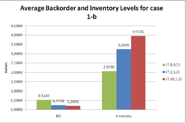
Table 4.5: Number of backordered demands and inventory levels for Case 1-b .... 49

Table 4.6: Total cost values of Case 1-b at each stage for each trial ... 49

Table 4.7: Trial values of Case 1-c ... 52

Table 4.8: WIP levels at each stage for Case 1-c ... 52

Table 4.9: Utilization rates at each stage for Case 1-c ... 52

Table 4.10: Backorders and inventory levels for Case 1-c ... 53

Table 4.11: Total cost of system for Case 1-c... 53

Table 4.12: The values of Case 1-d ... 56

Table 4.13: WIP levels at each stage for Case 1-d ... 56

Table 4.14: Utilization rates at each stage for Case 1-d... 56

Table 4.15: Backorders and inventory levels for Case 1-d ... 56

Table 4.16: Total costs of systems for Case 1-d ... 57

Table 4.17: The trial values of Case 2-a ... 60

Table 4.18: WIP levels at each station for Case 1-d ... 61

Table 4.19: Utilization rates at each station for Case 1-d ... 61

Table 4.20: Backorders and inventory levels of system for Case 2-a ... 61

Table 4.21: Total costs of system for Case 2-a ... 62

Table 4.22: Trial values of Case 2-b ... 65

Table 4.23: WIP levels at each stage for Case 2-b ... 65

Table 4.24: Utilization rates at each stage for Case 2-b... 65

Table 4.25: Backorders and inventory levels of Case 2-b... 65

Table 4.26: Total costs of systems for Case 2-b ... 66

Table 4.27: The trial values for Case2-c ... 69

Table 4.28: WIP levels at each stage for Case 2-c ... 69

viii

Table 4.30: Backorders and inventory levels of Case 2-c ... 70

Table 4.31: Total costs of systems in Case 2-c ... 70

Table 4.32: The trial values for Case2-d ... 73

Table 4.33: WIP levels at each stage for Case 2-d ... 73

Table 4.34: Utilization rates at each stage for Case 2-d... 73

Table 4.35: Backorders and inventory levels of Case 2-d... 73

Table 4.36: Total costs of systems for Case 2-d ... 74

Table 4.37: The trial values for Case3-a ... 77

Table 4.38: WIP levels at each stage for Case 3-a ... 78

Table 4.39: Utilization rates at each stage for Case 3-a ... 78

Table 4.40: Backorders and inventory levels of Case 3-a ... 78

Table 4.41: Total costs of systems in Case 3-a ... 78

Table 4.42: The trial values of Case 3-b ... 82

Table 4.43: WIP levels at each station for Case 3-b ... 82

Table 4.44: Utilization rates at each station for Case 3-b ... 82

Table 4.45: Backorders and inventory levels of Case 3-b... 82

Table 4.46: Total costs of systems in Case 3-b ... 83

Table 4.47: The trial values for Case 3-c ... 86

Table 4.48: WIP levels at each station for Case 3-c ... 86

Table 4.49: Utilization rates at each station for Case 3-c ... 86

Table 4.50: Backorders and inventory levels of Case 3-c ... 86

Table 4.51: Total costs of systems in Case 3-c ... 87

Table 4.52: The trial values for Case 3-d ... 90

Table 4.53: levels at each station for Case 3-d ... 90

Table 4.54: Utilization rates at each station for Case 3-d ... 90

Table 4.55: Backorders and inventory levels of Case 3-d... 90

Table 4.56: Total costs of systems in Case 3-d ... 91

Table 4.57: The trial values for Case 4-a ... 94

Table 4.58: WIP levels at each station for Case 4-a ... 94

Table 4.59: Utilization rates at each station for Case 4-a ... 95

Table 4.60: Backorders and inventory levels of system for Case 4-a ... 95

ix

Table 4.62: The trial values for Case 4-b ... 99

Table 4.63: WIP levels at each station for Case 4-b ... 99

Table 4.64: Utilization rates at each station for Case 4-b ... 99

Table 4.65: Backorders and inventory levels of system for Case 4-b ... 99

Table 4.66: Total costs of system for Case 4-b... 100

Table 4.67: The trial values for Case 4-c ... 102

Table 4.68: WIP levels at each station for Case 4-c ... 103

Table 4.69: Utilization rates at each station for Case 4-c ... 103

Table 4.70: Backorders and inventory levels of Case 4-c ... 103

Table 4.71: Total costs of systems in Case 4-c ... 103

Table 4.72: The trial values for Case 4-d ... 106

Table 4.73: WIP levels at each station for Case 4-d ... 107

Table 4.74: Utilization rates at each station for Case 4-d ... 107

Table 4.75: Backorders and inventory levels of Case 4-d... 107

x

LIST OF FIGURES

Figure 1.1: A picture of Kanban card ... 3

Figure 1.2: Schematic working method of a classical Kanban system ... 3

Figure 1.3: Schematic model of a sample CONWIP system ... 5

Figure 2.1: Single-card kanban, MRP, ROP, and the continuous system, in a continuoum. As it becomes harder to associate parts and end product demands, inventories likely increase-from theoritical zero on the extreme left to months’ worth on the extreme right. ... 9

Figure 2.2: Decomposition of the original system into r single-product subsystems. ... 15

Figure 2.3: Description Scheme of an e-kanban system ... 18

Figure 3.1: Algorithm of adaptive kanban system’s processing principles ... 26

Figure 3.2: Schematic model of a continuous time Markov Chain ... 28

Figure 3.3: A screenshot of the simulation model interface ... 29

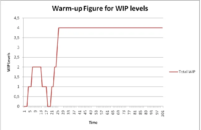
Figure 3.4: Warm-Up Figure For WIP Levels ... 31

Figure 3.5: Relation Curve between optimal kanban number and total cost in a kanban controlled production system ... 34

Figure 4.1: WIP Levels variations at each stage for Case 1-a ... 45

Figure 4.2: Average backorder and inventory variation for Case 1-a ... 46

Figure 4.3: Total costs variations of system for Case 1-a ... 47

Figure 4.4: WIP levels variation for Case 1-b ... 49

Figure 4.5: Average backorder and inventory variation for Case 1-b ... 50

Figure 4.6: Total Costs variations of system for Case 1-b ... 51

Figure 4.7: WIP levels variations at each station for Case 1-c ... 53

Figure 4.8: Average backorder and inventory levels variations for Case 1-c ... 54

Figure 4.9: Total costs variations of system for Case 1-c ... 55

xi

Figure 4.11: Average backorder and inventory variation for Case 1-d ... 58

Figure 4.12: Total costs variations of system for Case 1-d ... 59

Figure 4.13: WIP levels variations at each station for Case 2-a ... 62

Figure 4.14: Average backorder and inventory variation for Case 2-a ... 63

Figure 4.15: Total costs variation of system for Case 2-a ... 64

Figure 4.16: WIP levels variations at each station for Case 2-b ... 66

Figure 4.17: Average backorder and inventory variation for Case 2-b ... 67

Figure 4.18: Total costs variations of system for different trial values of Case 2-b 68 Figure 4.19: WIP levels variations at each station for Case 2-c ... 70

Figure 4.20: Average backorder and inventory variation for Case 2-c ... 71

Figure 4.21: Total costs variations of system for Case 2-c ... 72

Figure 4.22: WIP levels variations at each station for Case 2-d ... 74

Figure 4.23: Average backorder and inventory variation for Case 2-d ... 75

Figure 4.24: Total costs variations of system for Case 2-d ... 76

Figure 4.25: WIP levels variations at each station for Case 3-a ... 79

Figure 4.26: Average backorder and inventory variation for Case 3-a ... 80

Figure 4.27: Total costs variations of system for Case 3-a ... 81

Figure 4.28: WIP levels variations at each station for Case 3-b ... 83

Figure 4.29: Average backorder and inventory variation for Case 3-b ... 84

Figure 4.30: Total costs variations of system for Case 3-b ... 85

Figure 4.31: WIP levels variations at each station for Case 3-c ... 87

Figure 4.32: Average backorder and inventory variation for Case 3-c ... 88

Figure 4.33: Total costs variations of system for Case 3-c ... 89

Figure 4.34: WIP levels variations at each station for Case 3-d ... 91

Figure 4.35: Average backorder and inventory variations for Case 3-d ... 92

xii

Figure 4.37: WIP levels variations at each station for Case 4-a ... 96

Figure 4.38: Average backorder and inventory variations for Case 4-a ... 97

Figure 4.39: Total costs variations of system for Case 4-a ... 98

Figure 4.40: WIP levels variations at each station for Case 4-b ... 100

Figure 4.41: Average backorder and inventory variation for Case 4-b ... 101

Figure 4.42: Total costs variations of system for Case 4-b ... 102

Figure 4.43: WIP levels variations at each station for Case 4-c ... 104

Figure 4.44: Average backorder and inventory variation for Case 4-c ... 105

Figure 4.45: Total costs variations of system for Case 4-c ... 106

Figure 4.46: WIP levels variations at each station for Case 4-d ... 108

Figure 4.47: Average backorder and inventory variations for Case 4-d ... 109

xiii

LIST OF SYMBOLS

Production Rates at each stage : λP1, λP2 , λP3, λP4

Demand arrival rate : λD

Production rate of bottleneck workstation : rb

Random variate : U

Quantile function : F-1

Number of kanban cards : K

Starting value of kanban cards : K*

Number of extra kanban cards : E

Release threshold value : R

Capture threshold value : C

Number of kanbans in process at time t : N(t) Number of extra kanbans in process at time t : X(t) Demand arrival time for ith demand : Di

Production process time at jth station for kth order : Pjk

Inventory Levels : I

Penalty cost of average backordered demands : p

Average cost of work-in-process levels : WIPC Average cost of inventory levels : IC

Total cost of system : TC

Total time of simulation : T

Utilization Rate : u

Filled ith workstation : FilledWSi

Work In Process levels at each station : WIP1, WIP2, WIP3, WIP4

xiv

LIST OF ABBREVIATIONS

Just-In-Time : JIT

Constan work in process : CONWIP

Workstations : WS1, WS2, WS3,

WS4

Backorder Queue : BO

1. INTRODUCTION

1.1 INTRODUCTION

In manufacturing environment, there are different types of production control mechanisms. One of them is Just In Time (JIT) production systems which use demands as a signal for the production system. The main concept of JIT is to produce the product when it is needed and according to the requested amount. JIT systems help us to reduce setup times, improve the flow of products from warehouse to shelves and take advantage of employees more effectively. Since the production process is related to demand in JIT systems, if there is no demand there will be no production. Furthermore, JIT helps us to improve the importance of the relationship with the supplier. The expectation from JIT system is avoiding waste products and inventory, but especially decreasing the amount of inventory to zero, which is physically and practically impossible for production systems.

Even though the JIT systems have benefits, there are some missing links between theory and practice of JIT settings. JIT systems are designed for perfect conditions with stable demands, constant and balanced processing times, very low uncertainties and no breakdowns, but in real life cases there happen too much problems in the production process such as processing times variations, unexpected breakdowns, demand uncertainties. Many manufacturing companies which use JIT systems, are trying to avoid these uncertainties and increase efficiency of their production systems.

Considering the definition of JIT systems, we call the system ―pull production systems‖ since the systems use the demands as signal. Pull system is a kind of manufacturing method which controls the flow of resources by only using what has been demanded from system. In the pull systems, consumers request product and ―pull‖ it through the delivery channels. In these systems, the production process starts from the last stage, any demand starts the production process. The main characteristic of the pull systems is that production and distributions are demand-driven, and this enables producers to decrease lead times; however, pull systems are difficult to implement. Implementing

2

manufacturing systems is based on production control policies. ―In a manufacturing system at the shop-floor level, these control policies help to identify when to start and stop producing a product and when to switch from one product to another‖(Altıok 1996, pg.274).

―The single technique most closely associated with the JIT practices of the Japanese is the ―pull system‖ known as kanban developed at Toyota‖(Hopp, J. W. and Spearman, M. L.,2008, pg.168). Kanban system is a kind of production control system and Kanban means ―card‖ in Japanese. Kanban system is also known as Toyota’s production control system. This system is not an inventory control system, it is a system which tells manufacturers what to produce, when to produce and how much to produce by using the information on the cards. Using Kanban, manufacturers handle with the product and information flow together. There is no need for extra stock management. A Kanban card used in a factory is shown in Figure 1.1. As we see from the picture there is much information and data on the card. The information on a typical kanban card is as follows;

the stage where card is used the number of component the name of component the definition of component the kanban number

the name or the code number of the box which kanban card is regularly put in the workstation adress where Kanban card will be released. (the code number or the name).

3

Figure 1.1: A picture of Kanban card

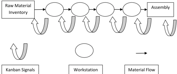
There are different types of Kanban systems in a manufacturing environment. Main Kanban concept is the classical Kanban system. In classical concept, when a demand enters the system, a part is removed from the system’s inventory point, then the workstation which feeds the inventory point sends an authorization signal to replace the part which was removed from inventory point. Then, each workstation does the same thing. Authorization signals are represented by Kanban cards. In the Kanban system, an operator requires both parts and an authorization signal (kanban) to work. A schematic working method of classical kanban system is shown in Figure 1.2.

According to figure 1.2, we can tell that there is one authorization signal only for the product but in Toyota’s kanban system, they make use of two types of cards to

Raw Material Inventory

Assembly

Kanban Signals Workstation Material Flow

4

authorize production and movement of product. Toyota’s two-card Kanban system’s schematic model is shown in Figure 1.3. As we mentioned before, classical kanban is designed for favorite conditions in a manufacturing environment. However, there exist systems which have uncertainties in systems’ performance measures such as demand or production process times. To avoid these uncertainties, many researchers, muanufacturing companies, academicians have tried to adapt the kanban systems to these uncertainties. In adaptive kanban systems, setting up the required kanban levels to avoid fill rates and related costs is complicated. That’s why, the aim of most of researches about JIT systems is to define the optimal solutions and measures for uncertainties in JIT systems and to specify how to design, monitor, and control kanban levels according to changes in demand, production capacity, and uncertainty levels to improve fill rate performance.

In genereal, the traditional kanban system is the most famous implementation of pull systems in which WIP levels are controlled at each station via cards but it’s not the simplest way for implementing the pull systems. To implement it easier, there is a variant which is named of kanban system which named Constant Work-in-process (CONWIP). CONWIP is a kind of single-stage kanban system which is easier to implement and adjust because in a traditional kanban system the production line uses cards for each product but in CONWIP the production line uses a set of cards for managing all the system. For sample, in a traditional kanban system to produce a finished item in the system there is a card for each part of the item, but in CONWIP system there is only one card which authorizes all parts of product. In figure 1.4, a scheme which shows a sample CONWIP system.

5

In manufacturing environment all companies which are using Kanban systems as production controlling policy try to adjust their system to real-life conditions. In that way academicians, researchers and companies do researches on production controling systems.

1.2 OBJECTIVE

The objective of this research is to develop a methodology to be used during the design of Kanban systems under uncertain conditions such as demand, lead time uncertainties. In this research a multi-stage, single-product CONWIP system is modeled and analyzed via simulation. The expectation is to decide how we can adjust a CONWIP kanban system to the uncertain conditions. Using extra kanban cards can help us to adjust the system at the right time or we can stabilize the production process against uncertainties, which helps us to save the cost of the system.

1.3 ORGANIZATION OF THE DISSERTATION

This research focuses on the effects of uncertainties on a single-card, single-product CONWIP based Kanban controlled production system. Chapter 2 represents a detailed literature review with the previous works which are focused on production control systems and policies. Chapter 3 describes the algorithms and formulas which are used for developing an sample model for analyzing the system. Chapter 4 represents the

Stock Point Authorization signals

6

simulation model, experimental cases and results which are analyzed via simulation. Chapter 5 represents the conclusion of all the results.

7

2. LITERATURE REVIEW

As we mentioned in Chapter 1, there are a lot of alternative production systems and control policies which are used in manufacturing environment. General alternatives are pull and push systems. Pull systems can be implemented in several ways. Kanban system is the most popular pull system in manufacturing environment, but kanban systems show their best performance under the ideal conditions such as stable demand, stable lead times, stable inter-arrival times between demands that create a missing link between theoritical and practical implementations of kanban systems. Due to this reason many researchers, academics or companies made a lot of research about how to implement kanban systems under the real-life conditions or how to reduce missing links between theoritical and practical implementations of a kanban system. Also there are different control policies such as base stock policy which is very easy to implement C. Duri et al. (2000).

From the point that there exist a lot of studies about Kanban systems with different algorithms and formulas Akturk & Erhun,(1999) made a literature review and classified different ways of determining design parameters and kanban sequences techniques for just in time systems. The important point is to state the relationships between design parameters which are number of kanbans, kanban sizes and scheduling decisions. The authors stated the relationships between parameters in a multi-item, multi-stage and multi-horizon kanban system. A model has been developed by authors to make some experiments for evaluating the impact of operational issues, like sequencing rules and actual lead times on design parameters. Methods which are used to determine design parameters have some steps such as model development, solution approaches, defining decision variables, defining performance measures, objectives of system, system’s configuration, type of kanban and the assumptions of model. The sample models are presented for sequencing production kanbans at each stage. Under different experimental conditions, sample models are analyzed. Analysis shows that none of the existing models of JIT considers the impact of operational issues on design parameters. There is a lack of different experimental kanban models for elaboration on scheduling kanban systems, these models have to work under different experimental conditions. Also, analysis which is done under different experimental conditions show that most

8

commonly used combination of First Come First Serve (FCFS) rule with instantaneous kanban withdrawal mechanism may not be a good policy all the time. FCFS rule performs better when the withdrawal cycle lengths are long enough for justifying setup times. By using four commonly used sequencing rules in literature Akturk & Erhun (1999) analyzed the impact of operational issues on design parameters.

As Akturk & Erhun (1999) mentioned in their detailed literature review, there are lots of different implementations of production control mechanisms. C. Duri et al. (2000) handled three different implementation types of production control systems and compared them with each other. They worked on make to stock pull control mechanisms such as kanban policy, base stock policy and generalized kanban policy which includes special cases of classical kanban and base stock policy. Authors noticed that the best known pull system is the kanban policy. This policy contains one design parameter per stage and for each type of product: the number of kanbans in stage. This parameter limits the maximum level of work-in-process (WIP) and finished parts inventory. The second policy is the base stock policy which includes one design parameter at each stage of system and for each type of product. Also base stock policy is very reactive. To show the characteristics of these policies with samples, authors made a quantitative comparison of these three control policies. These samples are analyzed with analytical methods for estimating the systems’ performance measures which depend on manufacturing processes, arrival process of external demands and parameters of different stages. For comparing three policies they designed three systems for each one of the policies. The authors noticed that optimization methods are not enough to analyze the generalized kanban system which is defined with design criteria of their work. These design criteria can be used by base stock and classical kanban because these systems are a kind of special case of generalized kanban system. They aimed at making a quantitative and qualititative comparison of three different pull mechanism production control systems, to choose the best policy to implement for controlling a production system and give practical rules to be used for choosing the system. Generally, their selection criteria is systems’ cost performances for the same production qualities under the same conditions. They show that if there is no delay in filling orders, all three policies have similar costs. However, if there is a delay in filling

9

orders, generalized kanban systems and base stock systems yield close to optimal costs that are lower than the costs of kanban system for the same production quality.

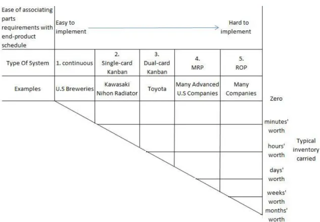
However, Duri et al. (2000) compared and analyzed different control policies such as kanban, generalized kanban and base stock systems. They did not consider the fact that there are different applications of production control policies. Schonberger Richard J. (1983) handled with different applications of kanban systems such as single-card and dual-card kanban systems. As we mentioned before, there are different implementations of kanban systems, one is single-card kanban system and the other one is dual-card kanban system which is known as Toyota production system. Schonberger defines kanban, push, and pull systems, and gives information about general characteristics of these systems such as where they are used, the ease of associating these systems, and any weak or powerful sides of theirs. Also, he showed a schematic comparison of different production control systems’ characteristics. In Figure 2.1, we can see the schematic model of these characteristics.

Figure 2.1: Single-card kanban, MRP, ROP, and the continuous system, in a continuoum. As it becomes harder to associate parts and end product demands, inventories likely increase-from theoritical zero on the extreme left to months’ worth on the extreme right.

10

Source: Rıchard J. Schonberger, (1983), “Applications Of Single-Card And Dual-Card Kanban”,

Production Scheduling, Materials Handling, 65.

He shows and makes criticism of different production control mechanisms and defines their characteristics in his work. Although there are different types of kanban in manufacturing environment, generally firms use classical kanban system, which can be single-product or multi-product kanban systems. This can create a difference between systems.

As we can see there are different pull production systems which are controlled by kanban cards in manufacturing environment. Woodruff et al. (1990) described a new pull based kanban system called CONWIP which means Constant Work-in-process. They compared the new system with classic kanban and push based production control of a single production line. They tell that CONWIP differs from Kanban in three main ways. These ways are as follows;

The use of backlog helps dictate the part number sequence,

cards are associated with all parts produced on a line rather than individual part numbers,

and jobs are pushed between workstations in series once they have authorized by a card to start at the beginning of the line.

They analyzed the new system by developing a simulated system. They have conducted numerous simulaitons to make comparisons between CONWIP and push based systems. They discuss the results of simulation study that illustrates some of advantages of CONWIP over a push based system. The system does offer some distinct advantages over kanban. For example, CONWIP can be used in some production environments where using classical kanban is not effective and practical because of too many part numbers or because of significant setups.

CONWIP concept has been used in different studies for solving different problems in pull production systems. Sarah M. Ryan et al. (1998) conducted a research on controlling a job shop setting within the concept of CONWIP. They tried to solve the problem of determining fixed overall WIP level to meet a uniformly high customer service requirement for all types of product and optimizing a queuing network model in

11

which orders pull completed product from the system. Under assumptions of heavy demand there is a throughput target for each product type. A simple heuristic has been provided for finding minimum total WIP and WIP (mix) which will achieve throughput through operating close to the throughput target. WIP (mix) is mixed WIP for all types of product. They focused on the proportion of orders which wait to be fulfilled by the production system. They worked on the problem to make a card count for each type of product so that the probability of waiting for an order to be fulfilled can be lower according to the production capacity. As a result, a higher total throughput could have been achieved without product mix constraint, but resulting system design would greatly favor orders for some products at the expense of others.

We know that a production system can produce single or multiple product also kanban systems can be single or multi product kanban systems. Schonberger Richard J. (1983) handled this subject but he didn’t analyze a sample model, he only defined the characteristics of the system and made criticism about the systems. C. Duri et al. (1995) concerned a kanban system analysis which produces several types of products. Also, they present an analytical method for analyzing the performance of a multi-product kanban system with using a closed multi-class queuing network model which each class represents one type of kanban. The system produces two types of products on the same machine so this creates ordering problem, which product would be the first. The setup times can be distinguishing characteristic for defining processing orders. There are two cases: the first one is; if setup times are not zero, we have to try to limit the number of setup, but if setup times are zero, we can choose and define processing orders. Therefore, there is no need to worry about setups number limitation. They focused on the second case for analyzing the system performance. They aimed at approximating an analytical method for analyzing the speed and accuracy for designing of a multi-product kanban system where they need to test numerous configurations of systems for selecting the best one to use in real-life production systems.

In a kanban system, one of the most important performance measure is Kanban sizes. Setting up kanban sizes in a production system is very important but we have to know the factors which influence the number of kanbans in a kanban controlled production system. Philpoom et al. (1987) made an investigation to identify these factors. The factors which they tried to identify include throughput velocity, coefficient of variations

12

in procesing times, the machine utilization and autocorrelation of processing times. All these factors are analyzed by using a simulation model. In a pull system, the system’s efficiency is measured with number of containers which include finished goods produced and stored, it means that more inventory is equal lower efficiency. When the authors analyzed the factors that influence the number of kanbans, they assume that one workcentre encompasses only one machine, and the system produces only one product in each processing time. Conveyance time and kanban collecting time are all zero or relative to processing time, also setup times are all zero and all processing times are equal. Analysis of sample simulation models show that if variability in processing times increase, the number of kanbans increase too. If the machine utilization increases, the number of kanbans increase and correlation of processing times have the same effect as other parameters.

While we design a production system, we have to choose system options carefully. To take the best performance results from the designed system, the system options have to be close to the real life production system options. In this respect, Deleersnyder (1989) noticed that there are three problems in designing and implementing a kanban controlled JIT system such as followings;

1. the identification of flow lines which is important for achieving the flow lines operating around the production families with a good level of utilization but with a minimal extra investment,

2. loading flow lines, which is important for avoiding bottlenecks developing in work stations,

3. controlling the operations, which is important for controlling the interaction between production and inventory levels and for determining the expected number of kanbans in systems under stochastic conditions.

They developed a 3 stage serial production model based on N-stage serial production systems. Also, the system is developed as a discrete time Markov model. They described their models with 4 levels which are variability in number of kanbans, the impact of machine reliability, the impact of demand variability and the impact of safety stock in the system. The system performance analyses are based on three sources which are; uncertainties of machine reliabilities, capaciy constraints and uncertainty of

13

demand. They aimed at analyzing a sample kanban based production system under these sources. They tested the effect of the number of kanbans variations on the system’s performance parameters such as average total inventory, average backlog, variance backlog, % lost demand, average job flow time. As a result, until the number of kanbans become 15, there is a small increase in all the performance parameters except average total inventory, but when the number of kanbans become more than 15, the effect on performance parameters will be dramatically bigger. When the production system becomes more reliable the average backlog decreases, this is the result of changing production reliability and the overall system performance. Also, the impact of demand variability makes the system more sensitive. Another result of the system is that while number of kanbans and safety stock increases, the average backlog decreases and average total inventory increases.

For analyzing the kanban production systems’ performance, there are a lot of models developed, but the analysis methods are different from each other. For sample as we noticed before, Deleersnyder et al. (1989) analyzed his model in a whole perspective. Also, Di Mascolo et al. (1996) used a different method to analyze the performance of a kanban system. They developed a general purpose of analytical method for analyzing the performance of multi-stage kanban controlled production system by using decomposition method. They considered single type production system and decomposed this system into stages in series. The basic principle of decomposing a system is to decompose main system into subsytems. They used a product form approximation technique for each subsystem’s analysis in isolation, after that an iterative procedure is used for determining the unknown parameters such as the percentage of demands that are backordered (not immediately satisfied), average waiting time of backordered demands and average work-in-process. The authors modeled the system as a queuing network. They analyzed the system for presenting the problems of single-stage and multi-stage systems. After the analysis of models, they first focused on the production capacity of the system because it’s the system’s maximum throughput. In the system developed in this work demand always comes to system for finished parts. As a result of the analysis, they noticed that production capacity increases with the number of kanbans at each stage.

14

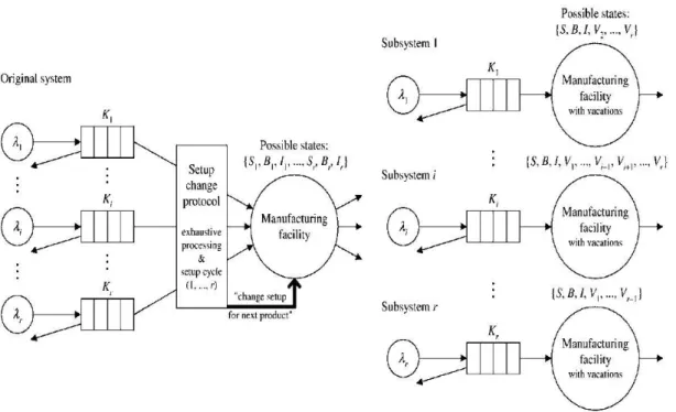
On the contrary to Di Mascolo et al. (1996), Krieg Georg N.&K. Heinrich(2004) developed a decomposition based method that analyzes and generates accurate estimates for steady-state performance measures of a kanban production system. A sample model of kanban system which can produce multi-product is developed. In the sample system, the setup and processing times are assumed to be exponentially distributed. According to mutually independent Poisson process, customers arrive to system. There is a target inventory level given by the number of kanbans. When the number of productions reach the target inventory level, the facility stops and setup for the next product according to a fixed setup sequence if the next product inventory is below target. Otherwise, this product is shipped. Also, when all products are at their target level, the facility idles. Another point in the system when a customer arrives to system, if there is no product in the inventory of the product which customer orders, customer satisfies his demand elsewhere, it is named as ―Lost Sales‖. According to Continuous Time Markov Chain algorithms; for a system which has five different products and five kanbans, systtem has 64805 states. For another system with 10 different products and 10 kanbans for each of them, the number of state is greater than 471 billion, as a result of this state space explosion, exact analysis of a model is mathematically not possible even for smaller systems. In this work as an alternative method the authors used decompositon method. Krieg &Kuhn (2004) decomposing figure can be seen in Figure 2.2.

15

Figure 2.2: Decomposition of the original system into r single-product subsystems.

Soruce: Georg N. Krıeg, Heınrıch Kuhn, (2004), “Analysis Of Multi-Product Kanban Systems With State-Dependent Setups And Lost Sales”, Annals Of Operations Research 125, 145.

The number of kanbans play a major role in the performance of kanban controlled production systems. Bard & Golany (1991) has developed a single-card production system which the empty containers function as kanbans and are used to trigger orders. They developed the system which is designed for a given demand and planning horizon. This sample model is very general, it is committing the problem in a wide range. The first and most important interest of the authors is the number of kanbans in the system. They made some assumptions that there is precisely one kanban of each product type for each container, the number of kanbans are equal to the number of containers and for each part it should be minimized, the containers which are used in the system have to be standard and must always be filled with the prescribed quantity. They also assumed that the production and withdrawal can be started only by appropriate kanbans. They aimed at minimizing holding and shortage costs without ignoring the basic kanban principles and balancing these costs over the planning horizon. They think that this system and algorithm may help assist line managers in determining optimal kanban numbers at each workstation. As a result, they noticed that this system is the most appropriate when demand is steady and lead times are short. Making careful analysis can yield immediate

16

benefits by reducing inventories and provide managers with a more detailed picture of current activites.

Determining the number of kanbans and analyzing its effects can be done by different methodologies for different systems. Markham et al. (1998) made a rule induction for using the number of kanbans in a JIT system by using a classification and regression tree (CART) technique which is developed by Briemen et al. (1984). If the production system is under ideal conditions such as stable demand, low process times, welltrained workers, there is no need for an adjustment on the number of kanbans in the system. However, in real life conditions it is impossible to make every condition ideal. From this point, they presented a methodology which allows the shop floor manager to identify the relationships between shop factors which need to be monitored if the firm’s aim is to operate its shop at least cost production kanban level in the near future. The methodology has been used on a sample in three steps which are data collecting, formation of desicion tree and interpretation of decision tree. There is a simple heuristic they noticed as a result, if there exist a high demand variability in the current period and if the lead time in the previous period is short and vendor supply variability is high in the previous period, then only a few kanbans are required for the system. Also using CART in a rule induction provides us with a viable solution to the knowledge acquisition bottleneck.

As a case study about Kanban controlled production systems Orbak & Bilgin (2005) conducted a research about Kanban systems. They tried to apply Kanban system in a small automotive raw part manufacturing company. Before starting to implement Kanban system, in a firm there are important things to do. These things are processing times’ standardization, reducing setup times, setting up the utilities according to JIT philosophy, total quality management applications for JIT systems such as the targets which are zero inventory and zero waste product. According to the firm’s production procedure they get data to analyze the system. The data includes average mean of demand interval, setup times, lead times, the number of lots produced, having inventory cost and not having an inventory cost. Considering the data collected by using Monden’s formula which has been described by Monden (1993), the authors tried to determine the optimal number of kanbans which get the system to minimize the costs. As a result of these calculations, they noticed that implementing kanban system in this

17

firm causes a decrease in counts of inventory with a rate of 50%, a decrease in counts of lots and this causes to an increase of lead times. Kanban system implementation gives company a lot of advantages to firm such as controlling defects quickly, decrease in waste products. Also, the production process becomes easier to understand and implement, and over-production is prevented. In a phrase, this study showed us implementing kanban system to a production system make production system easier and provide production managers with an easier control of system.

Generally researchers make assumptions about analyzing and designing a production sytem on the given kanban sizes. Chan (2001) tried to investigate the effect of kanban size variations on the performance of JIT manufacturing systems. There exist two types of JIT production systems; one is pull-type, the other one is hybrid type. These are analyzed by using computer simulation models. Author considered some performance measures such as fill rate, inprocess inventory and manufacturing lead time. Also, some other parameters such as demand rate, processing times are taken into consideration. He developed two simulation models for testing the effect of kanban sizes on different JIT systems. He aimed at determining optimal kanban size for optimizing the performance of system in terms of lead time and fill rate. As a result of single product system performance analysis while kanban size increases, fill rate decreases but inprocess inventory and manufacturing lead time increase. For multi product system analysis, he noticed while kanban size increases fill rate increases, too. However, manufacturing lead time decreases in the system when kanban size of system increases.

As a case study about Kanban controlled production systems Orbak & Bilgin (2005) conducted a research about Kanban systems. They tried to apply Kanban system in a small automotive raw part manufacturing company. Before starting to implement Kanban system, in a firm there are important things to do. These things are processing times’ standardization, reducing setup times, setting up the utilities according to JIT philosophy, total quality management applications for JIT systems such as the targets which are zero inventory and zero waste product. According to the firm’s production procedure they get data to analyze the system. The data includes average mean of demand interval, setup times, lead times, the number of lots produced, having inventory cost and not having an inventory cost. Considering the data collected by using Monden’s formula which has been described by Monden (1993), the authors tried to

18

determine the optimal number of kanbans which get the system to minimize the costs. As a result of these calculations, they noticed that implementing kanban system in this firm causes a decrease in counts of inventory with a rate of 50%, a decrease in counts of lots and this causes to an increase of lead times. Kanban system implementation gives company a lot of advantages to firm such as controlling defects quickly, decrease in waste products. Also, the production process becomes easier to understand and implement, and over-production is prevented. In a phrase, this study showed us implementing kanban system to a production system make production system easier and provide production managers with an easier control of system.

As we mentioned before, changing the number of kanbans in a kanban system is a big problem. Considering this problem Toyota Motor Corporation developed a new kanban system called ―e-Kanban‖ which utilizes computers and a communication network established between Toyota and its suppliers. Kotani (2007) makes a description of e-Kanban system which we can see in Figure 2.3.

Figure 2.3: Description Scheme of an e-kanban system

Source: Kotani, S.(2007) 'Optimal Method For Changing The Number Of Kanbans İn The <i>e</i>-Kanban System And İts Applications', International Journal Of Production Research, 45: 24, 5792

From the point that one goal of e-kanban system is improving the method which is used to change the number of kanbans, the author investigated a means of achieving this and proposed an optimal method for changing the number of kanbans. There are some improvements which are the result of implementing e-Kanban system. These are greater efficiency in the control of kanbans, reduced fluctuation in order quantity and appropriate changes in the number of kanbans, reduced parts inventories and quick

19

response to changes in demand. Also, applying this method to e-kanban system showed us e-Kanban system can manage parts ordering and delivery activities more efficiently and effectively than kanban system.

We know that there is a missing link between theory and practical applications of JIT systems. Theoretically implementing JIT system can be the best choice for a manufacturer but practically it’s hard to implement because in real life cases the manufacturing environment is very dynamic. Also, adapting the JIT systems to dynamic manufacturing environment is very important for the implementation of JIT systems. According to the idea of adapting JIT systems to dynamic environment Gupta & Al Turki (1997) developed a new system which uses an algorithm for manipulating the number of kanbans. They called the new system as ―Flexible Kanban System (FKS)‖. Gupta et al. (1995) noticed that FKS is a system which is quite robust and its performance is superior to TKS even for high processing times. In FKS, the idea is to increase the flow of production by reducing the blocking and starvation caused by the variability in processing times. This is achieved by increasing the number of kanbans in the system. FKS can increase or decrease the number of kanbans according to a base level number of kanbans, the system can’t reduce the number of kanbans below the base level. They developed a simulation model and analyzed it under the conditions that manufacturing system is composed by 8 stages, there is a demand for finished goods between 140 and 260 units for a planning horizon which is formed from 10 days, at every station processing times are independent and normally distributed, base level of number of production kanbans and withdrawal kanbans are set at two for each station, and transition times are 30 seconds for all kanbans. Also, to work on the sample model simulation they assumed that at station 1 there are always raw material available, each container includes one part, for producing one unit of demand raw material have to be processed at each station and first come first serve queuing discipline is used for processing the parts. For four performance measures which are time in system (TIS), work-in-process (WIP), average order completion time (OCT), and total number of units backlog 20 replications are made. They made this analysis for TKS and FKS to make a comparison between them. As the results of analysis, they noticed that average time in the system for FKS is longer than TKS, the average work-in-process in FKS is higher than TKS, the average order completion time in TKS is longer than FKS and the

20

total number of units which are backlogged during 50 days are zero for FKS. They aimed at developing a flexible kanban system which reduces the backlogs in the system by manipulating the number of kanbans in the system under these assumptions. We can see that they succeeded that aim.

Another work about adapting kanban systems to dynamic manufacturing environment was done by Takahashi & Nakamura (1999). They propose a system that can detect unstable changes in demand by using Exponentially Weighted Moving Average (EWMA) charts, and determine the revision of buffer size for the detected unstable changes based on tradeoff between performance measures under stable conditions. They used simulation experiments for analyzing and comparing performance of proposed JIT ordering systems. JIT systems being used in this work are kanban system and the concurrent ordering system which has been modified by Takahashi et al. (1996). In the modified concurrent ordering system when a demand arrives from succeeding stage an order is released immediately at the production system. Concurrent ordering system includes only one kind of information which is about the demand arrival at the production system. Besides that information, minimum releasing orders are considered. Also base stock system which is investigated by Buzacott & Shantikumar (1993) is the same system as concurrent ordering system. They developed two multi-stage JIT production systems. One is Kanban based, the other one is concurrent ordering system based. They simulated the systems and they compared the results of simulations. The production systems have same assumptions that a standard product is produced, the demand has stable and unstable changes, interarrival time of demand is distributed stochastically with unstable changes in the mean but variance is constant, production time at each stage is distributed stochastically, transportation process between (n-1)st and nth stages is called nth transportation stage, each stage has two inventory points named before and after inventory points, backorder is allowed and buffer sizes and the number of kanbans are controlled dynamically for reacting unstable changes in demand. As a result of simulation analysis both system can react to the unstable changes. Under tight requirement for waiting time of demand, kanban system is more efficient. Also, total mean of WIP inventories in kanban system is less than the concurrent ordering system.

21

In another study about adaptive kanban systems, Tardif & Maaseidvaag (2001) developed a new adaptive kanban system. This system is able to determine when to release or reorder raw parts based on customer demands, inventory and backorders. In this work authors developed the system for a single-stage and single product system. The proposed system helps us evaluate the performance of the system where the demands arrive according to a Poisson process. There is an extra card inventory in the system but these cards are free and ready to enter to production units. There are capturing and releasing thresholds which help us to decide when we have to release an extra kanban card to production unit or when we have to capture an extra card from the system. They simulated a sample system and results show that this system is able to completely dominate the traditional kanban system under certain conditions.

For adapting kanban systems to unstable changes and dynamic manufacturing system, again Takahashi & Nakamura (2002) proposed a decentralized reactive kanban system. The system is a multi-stage production and transportation system which is controlled by kanban system with reactive buffer size controllers for each stage. Controllers can detect the unstable changes in demand from succeeding stage and adjust buffer size in response to unstable changes. Unstable changes in demand are detected by utilizing control charts. To develop the decentralized system, they decomposed a multi-stage production system and the performance of decomposed system is analyzed by simulation experiments under various stable demand conditions. Based on the results of decomposed system’s performance, they developed the decentralized reactive kanban system. The assumptions of the system are all the same with Takahashi & Nakamura (1996) work except one assumption. In the previous system they assumed that there is a constant variance of demand but in this work they assume the variance is unstable. They decomposed the systems which are developed in Takahashi & Nakamura (1996) such as the kanban and concurrent system. Again, they used EWMA charts to detect the unstable changes in demand from the succeeding stage. They simulated the sample system, analyzed it and compared with previous centralized systems. The results of analysis showed that the proposed system’s performance is similar to the previous systems. Kanban systems need small work-in-process inventories for satisfying the required level of mean waiting time of product demand than the centralized reactive systems.

22

There are different types of reactive kanban systems in literature. In one of reactive systems, unstable changes in demand are detected by using control charts, and in these systems kanban numbers and buffer sizes are adjusted according to detected unstable changes. Another reactive system is based on inventory levels but this system’s performance has not yet been analyzed. Therefore, Takahashi (2003) proposed two reactive systems for analyzing and comparing performances. One of the system is control chart based and the other one is inventory based. He designed a new inventory based reactive kanban system and analysed its performance. In the inventory based system, instead of monitoring time series data, he monitored the inventory level to detect unstable changes in demand and adjust number of kanbans according to detected changes. He compared three systems which are control chart based system which is developed by Takahashi & Nakamura (1999) and previous inventory based system which is developed by Tardiff & Maaseidvaag (2001) and new inventory based system developed by Takahashi (2003). All systems’ performances are analyzed for unstable changes in demand. Systems are developed under the same assumptions as we mentioned in Takahashi & Nakamura (1999). Performance measures for analysis are the mean waiting time of product demand and the total mean WIP inventories. Analyzing these three systems’ performance results showed that both the proposed inventory based and control chart based systems are designed to minimize total WIP while maintaining waiting time less then the required level. Also, he noticed that control chart based and inventory based systems are robust for unexpected unstable changes in demand. We can expect good performances from these systems by setting the parameters for severe conditions and considering three reactive systems. The control chart based system is the most effective system since it responds to unstable changes in demand. Performance analysis showed that in the proposed system which is inventory based, exponentially smoothed inventory levels are used to detect unstable changes in demand and that causes a delay in detecting unstable changes in demand, also this causes an increase in total WIP. In all of these three reactive systems, unstable changes occurs in demand but in real life unstable changes can occur in production time or capacity and in these systems the variance of demand is assumed to be constant but there can be unstable changes in the variance of the mean.

23

According to the probability of having unstable changes in the variance of the mean, Takahashi et al. (2004) proposed a reactive kanban system for multi-stage production systems with unstable changes in demand, not only in the mean but also in the variance. Their reactive system is very similar to previous reactive systems which are developed by Takahashi & Nakamura (2002) and the assumptions are the same as the previous system. We mentioned that in the previous system the authors analyzed the system by decomposing multi-stage system into the single stage systems. Systems’ performance measures are the mean waiting time of demand and total mean WIP inventories. For analyzing the systems’ performance, the time series data on demand are grouped into batches and the batch mean. And, variance are utilized to detect unstable changes in the mean and variance of demand. Grouping causes a delay on detecting unstable changes. The batch size in grouping and multiplier of EWMA charts have an important effect on the system’s performance. They noticed that because of delay in detecting unstable changes and controlling buffer size causes not to satisfy the required level of mean waiting time but this problem can be solved with holding a little safety stock at the final inventory point. The system which they developed is effective in reacting kanban system to unstable changes.

As we mentioned in the previous works about adaptive kanban systems, researchers used different analyzing methods and developed algorithms. Sivakumar & Shahabudeen (2009) developed a multi-stage kanban system which is adapted from a traditional and adaptive kanban system. They used genetic and simulated annealing algorithms used for setting the parameters of systems. They created different cases for analyzing the systems and as a difference from other adaptive systems in some cases their systems have parallel servers. The objective of the models is minimizing the costs of systems. The cost of the system is also a performance measure, and the other performance measure is the number of kanbans. The main characteristic and difference of this system is the algorithms being used such as genetic algorithm and simulated annealing algorithm. The numerical results of analysis showed that multi-stage adaptive kanban system gives a better performance than multi-stage traditional kanban system. Also using simulated annealing algorithm has a better performance on analyzing kanban systems than genetic algorithm.

24

As we see in literature, different algorithms, methods and systems have been developed and analyzed about kanban controlled production systems by different researchers. Our system shows similar characteristics with the work of Tardiff & Maaseidvaag (2001). Our system is a sample of adaptive kanban system and it is based on CONWIP concept. In literature some researchers analysed their system with mathematical algorithms, whereas some of them analysed with a simulation model of system. The performance of system was analysed with simulation model of system. The systems developed in the previous works were designed without blocking. Difference of our system from these previous works is in our system there can be blocking and our queues of the system are limited. Because of blocking and limited queue, we need a complex mathematical model, also to make our analysis easier we have conducted our analysis with simulation. All the methodologies used and the model can be seen in Chapter 3.

25

3. PROBLEM DESCRIPTION AND MODEL

3.1 PROBLEM AND SYSTEM DESCRIPTION

In the kanban controlled production systems the most important problem is adapting system to uncertain conditions. As we mentioned before, JIT systems show their best performance under favorable conditions such as certain demand, certain lead times, certain process times but in real-life cases most of these conditions are uncertain. According to these uncertain conditions we tried to develop an adaptive kanban controlled JIT production system.

We considered a multi-stage, single-product and single-card kanban system which works under CONWIP methodology. The system is formed by 4 serial workstations, and each Workstation acts as a single server, also all workstations include a queue of products which are waiting to be produced. Queue has a limited capacity. In our study, we consider each workstation has a queue that can hold at most 3 items. The number of kanban cards in the system can change according to current inventory and backorders. The Manufacturing process is represented by ―MP‖, the inventory is represented by ―I‖ in the system in which the containers of finished parts are holded, the queue of demand is represented by ―D‖, the queue BO contains backordered demands and the queue Total Waiting Work contains the jobs which are waiting to enter to Workstation 1 with its’ kanban card. The adaptive system uses K number of kanban cards and E number of extra cards. Initially, before a demand arrives to the system, the number of containers in the queue of I is equal to K. Before system starts producing, D and MP are empty. N(t) is the number of cards in use at time t. Also, let X(t) be the number of extra cards in use at time t. R represents the release threshold for adding an extra card and C represents capture threshold when one retrieves an extra card from circulation.