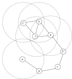
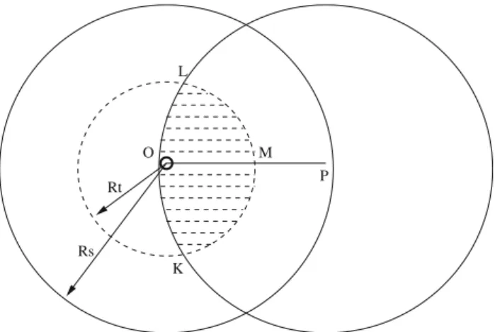
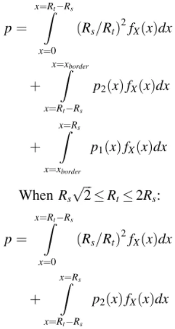
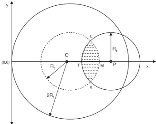
Sleep scheduling with expected common coverage in wireless sensor networks
Tam metin
Şekil


Benzer Belgeler
Doğalgazla ısıtmaya ek olarak, yaygın kullanılan bir sistem olan güneş enerjisi ile ısıtma sistemine göre toprak kaynaklı ısı pompası sistemi kullanımının
ve kullanılmıştır) öbürüyse Maiyet Köşkü (sultanın maiyeti, kimi zaman da haremi için kullanılmıştır) adlarıyla anılmış, ikisine birden de Ihlamur Kasrı
Tüm okuyucularımızı, Türk Kültürü ve Hacı Bektaş Velî Araştırma Merkezi olarak muharrem ayı içerisinde düzenleyeceğimiz faaliyetlerimize katılmaya davet ediyoruz..
En nihayet ikinci ve üçüncü de recede kalması icap eden hikâyeyi anlatan, nasıl büyümüş, tstanbu- lun nerelerinde oturmuş, evinin, sokağının tarifi hikâyeyi
(Hediye) İnşa 1218 Veli Ağa Yatay Dikdörtgen Prizma Kemer Sivri 208 x 514 Onarım 1313 Hacı Mehmed Baba. Üç Pınar Onarım
"D eniz ressamı” olarak ta nınan Ayvazovski’nin, dünyanın çeşitli müze ve galerilerinde sergilenen yapıtları arasında Anadolu kıyıları ve özellikle
Cumhur İttifakı’nın taraflarından birisi olan Tayyip Erdoğan’ın sahip olduğu karizmanın belki de en önemli özelliği, seçmeninin gözünde elit değil de, sıradan
Сталинград – это не просто город на Волге, он был для него символом Победы.. Это еще и главный военно-политический фактор Второй мировой войны; его
