GENERALIZATION OF TIME-FREQUENCY SIGNAL REPRESENTATIONS TO
JOINT FRACTIONAL FOURIER DOMAINS
Lutfiye Durak
∗, Ahmet Kemal ¨
Ozdemir
∗∗, Orhan Arikan
†, and Iickho Song
∗ ∗Department of Electrical EngineeringKorea Advanced Institute of Science and Technology 373-1 Guseong Dong, Yuseong Gu, Daejeon 305-701, Korea
[email protected], [email protected]
∗∗WesternGeco Ltd. Schlumberger House
Gatwick Airport, West Sussex RH6 0NZ, England [email protected]
†Department of Electrical Engineering
Bilkent University Ankara, 06800, Turkey [email protected]
ABSTRACT
The 2-D signal representations of variables rather than time and fre-quency have been proposed based on either Hermitian or unitary erators. As an alternative to the theoretical derivations based on op-erators, we propose a joint fractional domain signal representation (JFSR) based on an intuitive understanding from a time-frequency distribution constructing a 2-D function which designates the joint time and frequency content of signals. The JFSR of a signal is so de-signed that its projections on to the defining joint fractional Fourier domains give the modulus square of the fractional Fourier transform of the signal at the corresponding orders. We derive properties of the JFSR including its relations to quadratic time-frequency repre-sentations and fractional Fourier transformations. We present a fast algorithm to compute radial slices of the JFSR.
1. INTRODUCTION
Time-frequency representations are frequently utilized to analyze and process non-stationary signals [1, 2]. One of the major areas of research in time-frequency signal processing is the design of novel time-frequency representations for different applications. Unfortu-nately, time-frequency distributions do not always convey desirable qualifications in every application. Hence the demand for powerful signal representations has led to a substantial amount of research on the design of 2-D signal representations defined by alternative variables other than time and frequency. Joint time-scale represen-tations, which have attracted much interest especially in the fields of sonar and image processing, constitute one of the earliest exam-ples of this type of representations. Other popular choices of joint variables include higher derivatives of the instantaneous phase of signals for radar and sonar problems [3, 4], dispersive time-shifts for wave propagation problems and analogs of quantum mechan-ical quantities such as spin, angular momentum, and radial mo-mentum [5], and scale-hyperbolic time, warped time-frequency and warped time-scale.
These signal representations have been mathematically derived by using two alternative approaches which are both based on the operator theory: The variables are associated with either Hermitian operators as in [2] or unitary operators as in [5]. Recently, a joint fractional signal representation has been derived by associ-ating Hermitian fractional operators to fractional Fourier transform (FrFT) variables constituting the joint distribution [6]. The frac-tional Fourier domains are the set of all domains interpolating be-tween time and frequency. The fractional Fourier domains corre-sponding to a = 0 and a = 1 are the time and frequency domains,
respectively. The FrFT with order a transforms a signal into the
ath-order fractional Fourier domain and the ath-order FrFT of x(t)
is given by [7] xa(t) ≡ {Fax}(t) = Z Ba(t,t0)x(t0)dt0, −2 < a < 2, (1) where Ba(t,t0) =e −j(p sgn(a)/4+f/2) |sinf|1/2 ejp (t2cotf−2tt0cscf+t02cotf) (2)
is the transformation kernel,f =ap2 and sgn(·) is the sign function.
In this paper, we derive the joint fractional signal representation (JFSR) which designates the energy contents of signals in fractional Fourier domain variables instead of time and frequency. To this end, rather than using cumbersome mathematical equations based on operator theory, we extend our intuitive understanding from a time-frequency distribution, i.e., a function which designates joint time and frequency contents of signals. Then, we derive some im-portant properties of the JFSR including its relation to quadratic time-frequency representations and fractional Fourier transforma-tions, and present a simple formula for its oblique projections. We also present a fast algorithm to compute radial slices of the JFSR and numerically computed JFSRs of some synthetic signals.
The outline of the paper is as follows. In Section 2, a concise derivation of JFSR is presented as an alternative to the derivation given in [6]. Then, in Section 3, properties of the JFSR are exam-ined. After presenting a fast computation algorithm in Section 4, numerically computed JFSRs of some synthetic signals are shown in Section 5. Finally, conclusions are drawn in Section 6.
2. DISTRIBUTION OF SIGNAL ENERGY ON JOINT FRACTIONAL FOURIER DOMAINS
One of the primary expectations from a time-frequency distribution
Dx(t, f ) associated with a signal x(t) is that it accurately represents
the energy distribution of x(t). It is desired that the signal energy at
a frequency f for a time instant t is given by Dx(t, f ). Because of
the uncertainty relationship between time and frequency domains, it is impossible to satisfy this point-wise energy density requirement. Therefore, one is to be usually satisfied with a looser condition on the marginal densities
Z
Z
D(t, f )dt = |X( f )|2, (4) and integration of the distribution on the whole time-frequency
plane Z Z
D(t, f )dt d f = ||x||2. (5)
where X( f ) is the Fourier transform of x(t), and || · || denotes the L2
norm. One of the prominent energetic distributions which satisfy the desired relations (4) and (5) is the Wigner distribution (WD) which is defined as [2]
Wx(t, f ) =
Z
x(t +t/2)x∗(t −t/2)e−j2pftdt . (6) The WD of a signal can be roughly interpreted as an energy density of the signal, since it is real, covariant to time and frequency do-main translations and moreover signal energy in any extended
time-frequency region can be determined by integrating Wx(t, f ) over that
region [2]. Another nice property of the WD is that, its oblique pro-jections give the energy distribution with respect to the correspond-ing fractional Fourier domain [8]. Such properties and its ability to provide high time-frequency domain signal concentration make the WD attractive compared to other representations.
Although the WD and its enhanced versions are useful in time-frequency analysis, in some applications such as signal design and synthesis, it is more useful to have a time-fractional Fourier do-main representation. In a mathematical framework, by associating Hermitian operators to individual FrFT domains, a joint fractional representation of signals has been derived in [6].
In this section, the joint fractional domain signal representation (JFSR) is constructed using conditions similar to the ones given in
(3)-(5). Let the JFSR of a signal be denoted by Ea
x(u,v) where
a = (a1,a2)denotes the orders of fractional Fourier domains u and
v, respectively. It is desired that the marginal densities satisfy
Z
Exa(u,v)dv = |xa1(u)|2 (7)
and Z
Exa(u,v)du = |xa2(v)|2 (8)
where |xa1(u)|2 and |xa2(v)|2 are the energy contents of the signal
at the ath
1 and ath2 fractional Fourier domains, respectively. Similar
to (5), the overall integral on the u − v plane is desired to be
Z Z
Exa(u,v)du dv = ||x||2. (9) The conditions stated in (7), (8), and (9) make the JFSR a gen-eralization of the WD, since the JFSR reduces to the WD when (a1,a2) = (0,1).
To construct the distribution Ea
x(u,v) satisfying the conditions
on the marginal densities and the total energy, we make use of the projection property of the WD [8]
Z
Wx(ucosf −v sinf ,usinf +v cosf )dv = |xa(u)|2. (10)
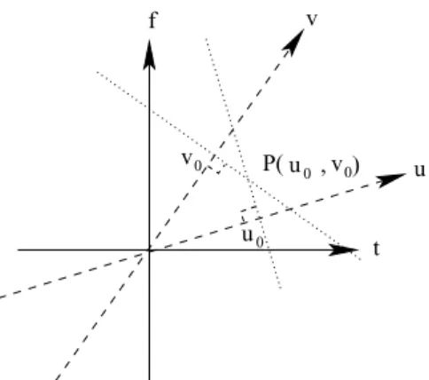
In Fig. 1, we observe that the value of the time-frequency distribu-tion at a point P contributes to the energy densities of the fracdistribu-tional
Fourier domains u and v at points u = u0and v = v0, respectively.
Therefore, the JFSR can simply be formed by redistributing the WD so that
Exa(u,v) = C ·Wx(P(t(u,v), f (u,v))) , (11)
where the coordinates (u,v) and (t, f ) are related by · cosf1 sinf1 cosf2 sinf2 ¸ · t f ¸ = · u v ¸ (12) 0 u v 0 P( , ) v 0 0 u u v t f
Figure 1: The value of the time-frequency distribution at a point P contributes to the energy densities of the fractional Fourier domains
u and v at points u = u0and v = v0, respectively. The JFSR can
simply be formed through redistributing the WD so that, Ea
x(u,v) = C ·Wx(P(t(u,v), f (u,v))).
andfi=aip/2 for i = 1,2. By using the total energy constraint (9),
the constant C in (11) is determined as
C = |csc(f12)| (13)
wheref12=f2−f1. Thus, Exa(u,v) is explicitly given by
|csc(f12)| Z x(usinf2−vsinf1 sinf12 +t/2)x ∗(usinf2−v sinf1 sinf12 −t/2)
×e−j2p t−ucossinff2+vcos12 f1dt .
An equivalent and more compact form of Ea
x(u,v) can be
ob-tained by using the rotation effect of the FrFT on the WD
Wxa1(u,v) = Wx(ucosf12−v sinf12,usinf12+v cosf12) , (14)
which verbally translates that WD of the ath1 order FrFT of a signal
x(t) is the same as the WD of the signal x(t) which is rotated by
f1radians in the clockwise direction in the time–frequency plane.
Consequently, Ea
x(u,v) can be derived in terms of the fractionally
Fourier transformed signal xa1(t) as
Exa(u,v) = Z xa1 µ u +tsinf12 2 ¶ x∗a1 µ u −tsinf12 2 ¶ × e−j2p(v−ucosf12)tdt (15) which has the same form as given in [6].
The JFSR can be generalized to define a cross-JFSR distribution of signals x(t) and y(t)
Exya(u,v) = |csc(f12)| ·Wxy(P(t(u,v), f (u,v))) (16)
= Z xa1 µ u +tsinf12 2 ¶ y∗ a1 µ u −t sinf12 2 ¶ × e−j2p(v−ucosf12)tdt . Defining Ea
x(u,v) through its relation to the WD provides an
easily interpretable definition of the JFSR of signals. From the def-inition given in (15), it follows that JFSR is a quadratic distribution while it is not a time-frequency distribution. Therefore it belongs to a broader class than the familiar Cohen’s class. Thus, its introduc-tion to the non-staintroduc-tionary signal processing will bring new insights into the design, filtering, analysis, and synthesis of signals in many applications.
3. PROPERTIES OF THE JFSR
In this section, we investigate the properties of the JFSR. In the properties listed below, the joint fractional Fourier domains have
the orders of a = (a1,a2)making angles of (f1,f2)with respect to
the time axis wherefi=aip2.
Property 1. The JFSR is a real distribution
Exa(u,v) = (Exa)∗(u,v) . (17)
Property 2. Orthogonal projection of the JFSR of a signal x(t)
on to u and v axes give the magnitude square of the FrFTs of the signal at orders associated with these axes: that is,
Z
Exa(u,v)dv = |xa1(u)|2 (18)
and Z
Ea
x(u,v)du = |xa2(v)|2. (19) Property 3. The area under the JFSR of a signal x(t) gives the
total signal energy
Z Z
Ea
x(u,v)dudv =
Z
|x(t)|2dt , (20) which follows from Property 2 and the unitarity of the FrFT.
Property 4 The JFSR and WD of a signal x(t) are related as
Ea x(u,v) = |cscf12|Wxa1 µ u,v − ucosf12 sinf12 ¶ = |cscf12|Wx µ usinf2−v sinf1 sinf12 , −ucosf2+v cosf1 sinf12 ¶ .
Property 5 The JFSR and the FrFT of a signal x(t) are related
as
Exaa0(u,v) = Exa+a0(u,v) (21)
where a + a0= (a
1+a0,a2+a0).
Proof: By using (21) in Property 4, the JFSR of xa(t) can be
written as Exaa0(u,v) = |cscf12| × Wxa0 µ usinf2−v sinf1 sinf12 , −ucosf2+vcosf1 sinf12 ¶ .
Then, by using the rotation property of the WD given in (14), right hand side of this expression is simplified to
Exaa0(u,v) = |cscf12|Wx(u 0,v0) u0 = usin(f 0+f2) −vsin(f 0+f1) sinf12 , v0 = −ucos(f0+f2) +vcos(f 0+f1) sinf12
which proves the property wheref 0=a0p
2.
Property 6 Any oblique projection of JFSR of a signal x(t) onto
an oblique axis making an angle off is
Pf[Exa](r) = |x(a0)(r/M)|2 , a0=2f
0
p , (22) where
f 0=arctan2(cosf
1+cosf +cosf2sinf ,sinf1cosf +sinf2sinf)
(23) and
M =p1 + sin2f cosf12. (24)
Proof: By the projection-slice theorem, the oblique projection
of the JFSR of x(t) at an anglef is given by
Pf[Exa](r) = Z Fx(z cosf ,z sinf )e−j2p zrdz , (25) where Fxa(z ,h ) = Z Z Exa(u,v)ej2p(zu+hv)dudv (26) is the radial slice of the 2–D inverse Fourier transform of the JFSR of x(t). By using (21), the following expression can be obtained for
Fx(a)(z,h )in terms of the ambiguity function Ax(.)of x(t) Fxa(z ,h ) =Ax(z cosf1+h cosf2,z sinf1+z sinf2) . (27)
Thus, the radial slice Fa
x(z cosf ,z sinf )of Fxa(z,h ) can be
ex-pressed as
Fa
x(z cosf,z sinf) =Ax(zM cosf0,zM sinf0) , (28)
wheref0 and M are as given in (23) and (24), respectively. It is
known that the radial slice of the ambiguity function of a signal x(t)
at the anglef has the following relation to the (a0)thFrFT of the
signal x(t)
Ax(z cosf0,z sinf 0) =
Z
|x(a0)(r)|2ej2p zrdr . (29)
Then, the relation in (22) can be obtained by combining (25), (28), and (29).
4. FAST COMPUTATION OF THE JFSR
In this section, we provide an efficient computation algorithm of the JFSR of a signal on arbitrary radial slices. Throughout the com-putations, we assume that the signal x(t) is scaled to x(t/s) before sampling, so that its WD is approximately confined into a circle of
radiusDx/2. Here, if the time-width and bandwidth of the signal
is approximatelyDtandD f, respectively, then the scaling
parame-ter s becomes s =pD f/Dtproviding a signal which has negligible
energy outside the interval [−Dx/2,Dx/2].
To compute the radial slice of the JFSR of a signal x(t), we use the relation
Exaa(r cosf,r sinf) = |cscf12|Wx(r cosf0,r sinf 0) (30)
where
f0=arctan(cosf cosf
2+sinf cosf1,cosf sinf2−sinf cosf1)
(31)
andf1andf2are the corresponding angles of the fractional Fourier
domains u and v with respect to the time axis. It has been shown
in [9] that the radial slice of the WD along the line (r cosf0,r sinf 0)
is Wx(r cosf0,r sinf 0) = Z x(a0−1) µ −l 2 ¶ x∗ (a0−1) µ l 2 ¶ e−j2prl dl . (32) Therefore, (30) and (32) can be used to construct the radial slice of
Ea xa(u,v) as Exaa(r cosf ,r sinf ) = |cscf12| Z x(a0−1) µ l 2 ¶ x∗(a0−1) µ −l 2 ¶ × e−j2prl dl . (33)
Figure 2: The JFSR of x(t) = e−p((t/3)2+0.3 jt3)
at joint fractional
Fourier domains with order (a) (a1,a2) = (0,0.25), (b) (a1,a2) =
(0,0.5), (c) (a1,a2) = (0,0.75), and (d) (a1,a2) = (0,1). The
distri-bution given in (d) is the same as the WD of x(t) since a1=0, a2=
1.
If the double-sided bandwidth of x(a0−1) is Dx and the
time-bandwidth product is N, then the integral in (33) can be discretized by Exaa(rDxcosf ,rDxsinf ) =|cscDf12| x N−1 k=−N q[k]e−j2Dpxrk (34) where q[k] = x(a0−1)[k]x∗(a0−1)[−k] and x(a0−1)[k] = x(a0−1)(k/(2D x))
is computed using the algorithm given in [10] with O(NlogN) com-putational complexity.
As the relationship (33) depends on the FrFTs of the signal x(t), computation of any M uniformly spaced samples on the line seg-ment r ∈ [ri,rf]along the radial slice of Exaa(rD xcosf,rDxsinf )can
be performed through the chirp-z transform algorithm in O((N +
M)log(N + M)) computational complexity [11]. In the following
section, the results of the algorithm are presented for a synthetic signal on various joint fractional Fourier planes.
5. SIMULATIONS
In this section, the JFSR of a quadratic frequency modulated (FM) signal which has a non-convex frequency support on the time-frequency plane are evaluated for four different joint fractional Fourier order pairs of a = (0,0.25), (0,0.5), (0,0.75), and (0,1).
The JFSRs of a quadratic FM signal x(t) = e−p((t/3)2+0.3 jt3)
which has a non-convex frequency support on the time-frequency plane are presented in Fig. 2. The distribution given in (d) with fractional Fourier order pair (0,1) is the same as the WD of
x(t). It is easier to observe the localization of the signal component
that depends on the order of the joint fractional Fourier domains. Because the uncertainty relation of the fractional Fourier domains has a tighter lower-bound when compared to the time and frequency domains [7].
6. CONCLUSIONS
A joint fractional domain signal representation is developed using the energy density interpretation of the WD on the time-frequency plane. The (u,v) axes defining the joint representation are chosen
as the a = (a1,a2)-th order fractional Fourier domains. The
dis-tribution is designed so that its projection of the JFSR on to the u
and v axes gives the modulus square of the fractional Fourier
trans-form of signals at the corresponding orders a1 and a2as |xa1(t)|2
and |xa2(t)|2, respectively. It is shown that the distribution Exa(u,v)
depends on the WD through a coordinate transformation. There-fore, the JFSR is a real-valued distribution, too. The overall integral of the JFSR on the (u,v) plane gives the total energy of the sig-nal. In this paper, as part of the novel results, oblique projections of the JFSR is also derived and a fast computation algorithm designed for the computation of arbitrary radial slices of the WD in [9] is extended to the computation of the JFSR. The JFSRs of various sig-nals at various fractionally-ordered domains are presented and the localization of the signal components are compared.
The JFSR cannot be analyzed in the framework of the famil-iar Cohen’s class. However, its introduction to the non-stationary signal processing will bring new insights into the design, filtering, analysis, and synthesis of signals.
Acknowledgement
This research was supported by Brain Korea 21 Project under a 2004 grant from the School of Information Technology, KAIST, for which the authors would like to express their thanks.
REFERENCES
[1] F. Hlawatsch and G. F. Boudreaux-Bartels, “Linear and
quadratic time–frequency signal representations,” IEEE
Sig-nal Process. Magazine, vol. 9, pp. 21–67, Apr. 1992.
[2] L. Cohen, Time–Frequency Analysis, Prentice Hall, Engle-wood Cliffs, 1995.
[3] S. Mann and S. Haykin, “The chirplet transform: Physical considerations,” IEEE Trans. Signal Process., vol. 43, pp. 2745–2761, Nov. 1995.
[4] R. G. Baraniuk and D. L. Jones, “Matrix formulation of the chirplet transform,” IEEE Trans. Signal Process., vol. 44, pp. 3129–3135, Dec. 1996.
[5] R. G. Baraniuk, “Beyond time-frequency analysis: Energy density in one and many dimensions,” IEEE Trans. Signal
Process., vol. 46, pp. 2305–2314, Sep. 1998.
[6] O. Akay and G. F. Boudreaux-Bartels, “Joint fractional signal representations,” Journal of the Franklin Institute, vol. 337, pp. 365–378, 2000.
[7] H. M. Ozaktas, Z. Zalevsky, and M. A. Kutay, The
Frac-tional Fourier Transform with Applications in Optics and Sig-nal Processing, John Wiley & Sons, New York, 2000.
[8] A. W. Lohmann and B. H. Soffer, “Relationships
be-tween the Radon–Wigner and fractional Fourier transforms,”
J. Opt. Soc. Am. A, vol. 11, pp. 1798–1801, June 1994.
[9] A. K. ¨Ozdemir and O. Arıkan, “Efficient computation of the ambiguity function and the Wigner distribution on arbitrary line segments,” IEEE Trans. Signal Process., vol. 49, pp. 381– 393, Feb. 2001.
[10] H. M. Ozaktas, O. Arıkan, M. A. Kutay, and G. Bozdagi, “Digital computation of the fractional Fourier transform,”
IEEE Trans. Signal Process., vol. 44, pp. 2141–2150, Sep.
1996.
[11] L. R. Rabiner, R. W. Schafer, and C. M. Rader, “The chirp z– transform algorithm and its applications,” Bell Syst. Tech. J., vol. 48, pp. 1249–1292, May 1969.