Performance analysis of two-level forward error correction for lostcell recovery in ATM networks

Performance Analysis of Two-Level Forward Error Correction for Lost Cell Recovery

in

ATM

Networks

Nihat Cem Oguz

Department of Electrical and Electronics Engineering Bilkent University

Bilkent, Ankara, 06533, Turkey

Abstract

The major source of errors in B-ISDN/ATM systems is ex- pected to be bufler over$ow during congested conditions, result- ing in ATM cell losses which degrade the qualiry of service. It has been shown by many authors that the performance of the end-to-end system can be made much less sensitive to cell loss by means of forward error correction. This paper discusses the use of a two-level forward error correction scheme for virtual chan- nel and virtual path connections in ATM networks. The scheme exploits simple block coding and code interleaving simultane- ously. The simple block, interleaved, and joint coding schemes are studied and analyzed by using a novel and accurate discrete- time analytical method which enables the burstiness of cell losses be captured precisely. Detailed performance calculations, which indicate that it is possible to reduce the cell loss rate by several orders of magnitude overa wide range of network loadfor various trafic conditions, are discussed, and compared with simulation results. The comparisons show that the method is very accurate for bursty trafic. The advantages of the three coding techniques are quant$ed for different trafic characteristics and scenarios.

1

Introduction

In ATM networks the end-to-end propagation time for a typi- cal connection will be much larger than the duration of a packet. Since each retransmission increases the delay of a packet by ap- proximately the round-trip propagation time, the delay-throughput performance deteriorates significantly if the conventional error de- tection and Automatic Repeat reQuest (ARQ) mechanisms are em- ployed to provide end-to-end reliability. This is intolerable espe- cially for delay-sensitive high-speed applications such as real-time video. The same problem is present in satellite and deep-space communications, where open-loop error correction techniques are preferred to ARQ [l]. In 1975, Maxemchuk suggested the use of Forward Error Correction (FEC) to reduce the end-to-end de- lay for datagram-based services [ 2 ] . In a similar manner, it has been suggested to use FEC in high-speed networks, in particular ATM networks, to improve reliability without increasing packet delay [3]-[ 121.

In ATM, the basic unit of transport, switching, and queueing is a 53-octet cell composed of a 5-octet header and a 48-octet information field [13]. Since optical fibers have very low error rates, cell loss due to buffer overflow will be the dominant source

Ender Ayanoglu AT&T Bell Laboratories 101 Crawfords Corner Road, 4F-507

Holmdel, NJ 07733-3030

of errors in ATh4 networks [6]. FEC for ATM, compensating for cell losses, can be achieved by introducing separate parity cells transmitted along with the information-bearing cells. By this redundancy, the receiver can restore transmitted data without requiring retransmissions. But, in competition with this recovery capability, the parity cells increase the network load, and in turn, the cell loss rate before recovery. Therefore, the FEC scheme should introduce a reasonable parity overhead and be still suffi- ciently powerful to overcome this increase, so that a significant net gain is achieved. As long as the positions of losses are known, employment of erasure correcting codes is desirable in this re- spect since these codes are more powerful (typically by a factor of two) than error correcting codes of the same redundancy [14]. The principal motivation of this work is the fact that an ef- fective FEC scheme for ATM networks should be tailored to congestion losses. Simple block coding over consecutive cells, i.e., appending h parity cells to every group of IC consecutive information-bearing cells to form frames of n = E

+

h cells, is

effective when losses are dispersed evenly over the cell stream (e.g., are random). Since ATM networks are intended to support a wide variety of services with different traffic characteristics in- cluding bursty ones, a congested buffer will remain congested for a sufficiently long period to last over several frames. Consequently, cell losses will be correlated in time, in other words, will occur in bursts. To be able to recover from burst cell losses, we intro- duce a second level of coding. In addition to simple block coding within individual frames (cell coding), we similarly append h’ par- ity frames to every group of E’ consecutive information-bearing

frames, and form coding blocks of n’ = E’

+

h’ frames (frame

coding). This is equivalent to interleaving n rate k‘/n’ codes over a rate k f n coded cell stream, and has been previously pro- posed in the particular form of adding one parity cell per frame and one parity frame per coding block [4]. This paper studies the performance of this joint cell-and-frame coding scheme, in addi- tion to cell-only and frame-only coding schemes, with a detailed analytical model.

With regard to performance evaluation, some of the previous work focused on cell-only C31, 141, [81, [IO], [ l l l , and some on frame-only coding schemes [5], [9]. Shacham and McKenney assumed independent cell losses to analyze the performance of cell-only coding with one parity cell per frame, and made simu- lations for the actual case of correlated cell losses showing that independent cell loss assumption in the analysis may yield overly optimistic results [3], [4]. Kitami and Tokizawa analyzed the performance of frame-only coding under the independent cell

loss assumption [5]. McAuley described a Reed-Solomon burst erasure coder based system for reliable broadband communica- tions [6], and Ayanoglu et al. discussedincorporation of FEC into high-speed protocols [7]. Zhang and Sarkies modeled a Virtual

Path (VP) as a tandem queueing network, and considering inter- rupted and Markov modulated Bemoulli cell sources, developed a Markov chain model to estimate the output buffer contention, and hence, the cell loss process characteristics [8], [lo]. Ohta and Kitami improved the analysis in [5] via a two-state Markov chain characterization of the cell loss process (the Gilbert loss model), and dealt mainly with the practical issues of obtaining end-to-end erasure channel for a VP connection [9]. Biersack carried out extensive simulations to show the effectiveness of cell-only cod- ing for an ATM traffic stream derived from a real, compressed motion picture interfering at a node with its time-shifted replicas as well as bursty cell streams [ 1 11. The results of [ 1 11 revealed that cell-only coding would not be adequate for bursty traffic, thus confirming the motivation of this work.

More recently, being motivated by high-speed services sen- sitive to both loss and delay, we considered a hybrid solution involving two-level FEC accompanied by ARQ [ 121. In this con- text, assuming ATM switches with dedicated and shared output queueing at the nodes, we simulated a four-node Krtual Chan-

nel (VC) connection in a highly bursty traffic environment, and

showed that two-level coding could significantly reduce frame retransmissions.

The primary goal of this paper is to study the effect of traffic characteristics on the coding performance and to demonstrate the usefulness of two-level coding. For this purpose, focusing on a delay-sensitive VC traffic traversing a single node, we compare the cell-only, frame-only, and joint cell-and-frame coding perfor- mances separately for random and bursty traffic cases, seeking the most suitable coding technique for each case.

The performance study is based on a new, discrete-time ana- lytical approach which has similarities to [8] and [IO]. It differs from [8] and [lo] mainly in that the buffer occupancy is char- acterized by a Markov chain with the burstiness of cell arrivals

explicitly incorporated into the model. Recently, Cidon et al. ex- ploited this idea to analyze the packet loss process for continuous- and discrete-time systems, but not completely described the par- ticular case of discrete-time system with multiple sources [15]. Although our model has higher complexity as compared to those of [8] and [lo], and also to the Gilbert loss model abstraction of [9] (especially higher in this case), it captures the bursty nature of the cell loss process precisely, and hence, allows accurate quantifica- tion of the cell and frame loss rates for the uncoded and coded cases by means of computational algorithms similar to those of [81, [IO], and [151.

2

The Two-Level FEC Scheme

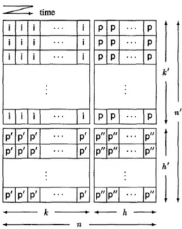
The two-level coding scheme is shown in Figure 1. Assume that cells fill a coding matrix row-wise as being transmitted. The FEC encoder generates h parity cells (p-cells) for every group of k consecutive information-bearing cells (i-cells). The p-cells are transmitted immediately after the kth i-cell of the correspond-

I

k’

p” p”

. . .

p” p”

.

.

.

-- k _____c c-h __c

.c--. n c

Figure 1: The two-level coding scheme.

ing row, under the control of a peak rate policing mechanism. Each one of the first k’ rows of the coding matrix constitutes an information-bearing frame. We refer to coding cells within a frame as cell coding. Similarly, h’ parity cells @’-cells) are gen- erated for every column of k’ i-cells, and buffered in respective h’ parity frames which are appended h p”-cells according to the cell coding rules. The parity frames are transmitted similarly after the last information-bearing frame. We would like to be able to use a p”-cell in both row and column decoding, therefore we consider systematic linear block codes. The p”-cells can also be generated by using the corresponding k’ p-cells according to the rules of coding over columns, which we refer to asframe coding.

We assume that the end-to-end connection can be viewed as an erasure channel. That is, the locations of lost cells in the coding matrix are known by the receiver. It is then possible to find optimal, maximum distance separable erasure correcting codes for both cell and frame coding so that the FEC decoder can recover up to h losses in a frame and h’ losses in a column [14]. In the simplest case of single-parity cell-only coding ( h = 1, h’ = 0), each bit in the payload of the p-cell is the modulo-2 sum of the corresponding bits of k i-cells. This p-cell can be constructed without any encoding delay by carrying out a bitwise modulo-2 addition on the i-cells as they are being transmitted. Since any cell in a frame is the bitwise modulo-2 sum of the remaining kcells, the decoder can easily make up for loss of one i-cell provided that its location is known. Multiple-parity coding involves manipulation of the information payloads of cells m bits taken at a time. Similar to the case of single-parity coding, there is no encoding delay due to the multiply-and-add nature of the encoding operation.

Observe that the two-level code allows recovery of up to

h’n

+

k’h lost cells out of nn’ provided that they are distributed

6b.3.2

over the coding matrix appropriately. In particular, loss of h’n consecutive cells, or complete loss of h’ frames can be compen-

sated for by frame coding if the number of losses in other frames does not exceed h per frame. Obviously, the most powerful code with the same parameters is the one that can recover any pattern of h’n

+

k’h lost cells out of nn’. This can be achieved by cell coding with

kk’

i-cells and h’n

+

k’h p-cells. However, the av-

erage decoding delay, i.e., the average time that a lost cell waits for a possible recovery, may then be too large. Furthermore, the higher the block length is, the higher the coding complexity will be. With the two-level coding approach, the recovery capability is structurally distributed over rows and columns of the n’ x n matrix, and we take the advantage of reduced code complexity at the expense of losing decoding flexibility. Also, the average decoding delay is reduced if decoding within a frame is done im- mediately upon detection of the frame boundary without waiting for the completion of the whole coding matrix.

The two-level FEC can be performed for both VC and VP connections as described in detail in [16].

3 Analytical Framework

In this section, we develop a discrete-time analytical frame- work to evaluate the performance of the two-level coding scheme for a VC connection. The tagged traffic belonging to this con- nection is assumed to traverse a single node at which it interferes with N

-

1 untagged traffic streams. Assuming that there is an

N x M ATM switch with dedicated output queueing at the node, and concentrating on the tagged output port, the node is modeled by an N-to-1 ATM multiplexer where the output buffer is a FIFO

queue of capacity B cells.

The main objective in our analytical approach is to obtain an accurate model for the tagged cell loss process. This requires the burstiness of the input traffic streams be incorporated into the model. For this purpose, considering discrete-time Markovian cell sources, we construct a Markov Chain (MC) for the buffer occupancy with the states of the tagged and aggregate untagged sources augmented explicitly into the state variable. For realis- tic N and B , this augmentation results in a very large MC as

compared to those of [8]-[lo], but it enables the burstiness of tagged cell losses be captured precisely, and hence, allows accu- rate quantification of the cell and frame loss rates by means of computational algorithms similar to those of [8], [lo], and [15]. For the sake of tractable time and memory complexity of these algorithms, we consider simpler sources than the interrupted and Markov modulated Bernoulli sources of [8] and [lo] so that the state transition probability matrix for the augmented MC becomes sparse. Yet these sources are capable of generating traffic streams of diverse characteristics.

We first discuss the input traffic model in Section 3.1. Then, the cell loss process model, i.e., the augmented MC, is introduced in Section 3.2. Based on this model, we obtain an approximate frame loss process characterization in Section 3.3. Finally, in Section 3.4, the computation of the cell and frame loss rates is discussed. In these computations, we assume that the end-to-end systemoperates properly, i.e., the receiver can always identify the

q1,m =

_{= P}

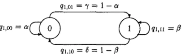
Figure 2: MC model of one source.

lost cells.

3.1

Input

Traffic

Model

We consider N independent discrete-time Markovian cell sources at the input of the multiplexer, which have identical statis- tics when there is no coding. The MC model of one source is shown in Figure 2, where the states 0 and 1 correspond respec- tively to the “idle” and “active” states of the source.

The state transitions occur once per slot, which is the unit time required to transmit a cell over the output link, and a source generates one cell per slot when it is active. Therefore, the steady state probability for the active state, given by

p1 = (1 - a ) / @

-

a -

P ) ,

is the normalized load offered by one source. Consequently, the normalized aggregate load becomes

N

P = P I = N p i

m= 1

since the sources are independent and identical for the no coding case.

When the tagged traffic is coded as described in Section 2,

the Markovian behavior of Figure 2 is no longer valid due to the periodic insertion of parity cells. However, we assume that this behavior is preserved even after the encoding operation, and reflect the effect of parity overhead in the traffic parameter ,L3 only so that the effective normalized tagged load becomes

P e t = pl(1

+

h / k ) ( l + h ’ / k ’ ) . ₍₃₎

That is, the probability distribution of idle duration for the tagged source is not affected by parity cell insertion. This is reasonable due to the memoryless property of the underlying discrete-time geometric random process.

Superposition of M = N - 1

>

1 independent and identical untagged sources results in an aggregate source, which is modeled by an ( M

+

1)-state discrete-time MC. The state variable is the number of active untagged sources, or equivalently, the number of simultaneous untagged cells. The subscript 1 in q1,ij of Figure 2 is attributed to the single source. With similar notation, let q M , i j , a, J = 0, 1,2, . . .

,

M , be the state transition probabilities for this

MC. Observe that a transition from state a to state j occurs when

I of i active sources become idle, and j

-

( i

-

I) of M

-

i

idle sources become active simultaneously in a slot. Therefore, we

(a

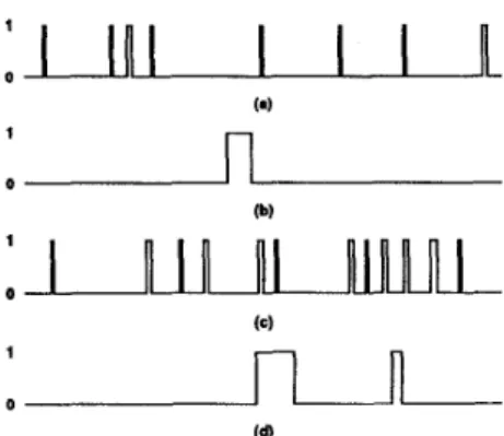
Figure 3: Some typical cell stream realizations over 200-slot periods for the following offered loads and clustering coefficients: (a) p1 = 0.05, c = 1.2; (b) p1 = 0.05, c = 1.9; (c) pi = 0.1,

c = 1.2; and (d) p l = 0.1, c = 1.9. Cells generated consecutively are represented by a single pulse of height 1 and width proportional to the number of cells in the batch.

have

where

1

= max(0, i - j) and

i

= min(i, M

-

j ) . It can be shown that (4) reduces to the transition probabilities of Figure 2 when M = l .

Observe that a source as just described generates a correlated, or bursty, traffic in general. However, when cy

+

/3

= 1, we have a simple independent Bernoulli process since ql,w = q1,lo

and q1,11 = q1,01, and a completely uncorrelated cell stream is

generated. Let

be the clustering coeficient which serves as a measure of the burstiness of a source when the offered load is small. In general, the closer c to 2 is, the burstier the source becomes. For example, when pl E (0,0.1], (1) and ( 5 ) imply cy E [0.92,1) and

/3

E (0.2,0.28] for c = 1.2, meaning that cell arrivals tend to be dispersed over time. On the other hand, we have cy E [0.99,1) and /3

E

(0.9,0.91] for c = 1.9, and cells are likelier to arrive in clusters. In Figure 3, the typical cell stream realizations obtained over 200-slot periods for the offered loads p1 = 0.05 and p1 = 0.1 illustrate the respective random and bursty characteristics for c = 1.2 and c = 1.9, thus proving the capability of the sources we consider to generate traffic streams of diverse characteristics.

c L + p E (0,2) ( 5 )

3.2

Cell Loss Process Characterization

Given the tagged and untaggedtraffic parameters, to character- ize the cell loss process for the tagged VC connection accurately without ignoring the burstiness of cell arrivals, we construct a 3-

Dimensional (3-D) discrete-time MC model for the buffer, which

is driven by 1 tagged and N

-

1 untagged cell sources. The state variable is the

(a,

t , U ) triplet, where t E ( 0 , l ) is the state of the tagged source, U E (0, 1,2,.

.

.

,

N

-

1) is the number of

active untagged sources, and b E {0,1,2,.

.

. ,

B } is the buffer occupancy after t

+

U new cells arrive in a slot. The multiplexer is assumed to be intemally non-blocking and capable of trans- porting all the simultaneous input cells to the buffer in zero time. If the buffer is empty, a randomly chosen one of the new cells is transmitted immediately over the output link, and the rest is stored in random order. Otherwise, the leading cell in the buffer is transmitted first, and the new cells are stored in random order again, provided that there is enough room for them. Therefore, the buffer occupancy is characterized by the relation

b, = min ( B , max(0, b , - l

+

t ,

+

u s

-

1)) (6) where the index s is the slot variable.

Observe that there are 2 N ( B

+

1) distinct ( b , t , a) triplets. However, some of them are inconsistent: they correspond to transient states due to the boundary conditions at b = 0 and

b = B. It follows from (6) that

( i ) if b,

<

B , t ,

+

u s

>

b8

+

1 implies that b,-1

<

0, or more than one cells are transmitted over the output link in slot s; and,

(ii) ifb, = B , t s + u d =Oimpliesthatb,-l

>

B,orthebuffer remains full although no new cells arrive in slot s. Discarding these transient states, we have the following irre- ducible state space:

S = { ( b , t , u ) : t + u

5

b + 1 if b

<

B,and

t

+

U

>

0 if b = B}. ₍₇₎

Since b in the ( b ,

t ,

U ) triplet is dependent on

t

and U , the state transition probabilities of the 3-D MC follow from those for t and u given by (4). That is, in a slot, a transition from ( b , t , U ) E S to (b’, t’, U’) E S occurs with probability ql,ttjqN--l,uu’ if

b’ = min ( B , max (0, b

+

t’

+

U‘

-

1)), and with probability 0 otherwise.

Suppose that we are in state ( b , t , U ) E S at the end of a slot. Then, the maximum number of new cells that can be served in the nextslot is B

-

b + 1. Therefore,if there are t’+ U’

>

B

-

b + 1 new cell anivals, randomly chosen t’

+

U’

-

( B

-

b

+

1) of them are lost. In particular if t‘ = 1 and U ’

>

B

-

b, the tagged cell is lost with probability 1

-

(B

-

b

+

1)/( 1 +U’), and the new state becomes (B, 1, U ’ ) . We distinguish the potentially “bad” states

( B , 1, U’) with U’

2

1 from the others, and decompose each oneinto two states (B, 1, U’) and (B, 1, U’)*, which respectively indicate tagged cell “success” and “loss.” This decomposition is

illustrated in Figure 4 where it is assumed that U’

>

B

-

b. Let

SL

be the set of tagged cell ‘‘loss’’ states, i.e.,

SL = { ( B , 1 , U ) * : u = 1 , 2 , .

.

. ,

N

-

1). (8)

Then, we have the extended 3-D MC with state space S E =

S U

SL

.

For

i,

j E S E , let pi j be the transition probability from state

i

to state j , and p , be the steady state probability of state i.

For B

2

N

-

2, it can be shown that the number of states in S E

is

(9) Therefore, l S ~ l gets very large for realistic N and B. For ex- ample, when N = 16 and B = 100, we have I S E ~ = 3021,

ISEI

= 2 N ( B + 1)

-

( N 2

-

3 N + 3 ) .

6b.3.4

potentially “bad” state tagged cell “success” tagged cell “loss” Figure 4: Decomposition of a potentially “bad“ state into tagged cell “success” and “loss” states.

and the solution for pi, i E SE, may seem infeasible. However, the number of states reachable from any state in SE in just one transition is limited to be at most 3 N

-

1 in the worst case of reachable subset containing all of the tagged cell “loss” states. This means that the state transition probability matrix for SE is sparse for large B , and consequently, the problem is of tractable complexity with respect to both time and memory requirements.

Observe that this model captures the burstiness of the traffic streams, and hence, constitutes a basis for accurate study of the effectiveness of the two-level FEC scheme. For this purpose, let { F ( v , n) : v = 0, 1,2,.

. . ,

n} be the Cell Loss Pattern Distri- bution (CLPD), where F ( v , n) is the probability of v losses in a frame of n tagged cells. To compute the CLPD, we partition S into two subspaces

(10) and

(1 1) where

SD

is the set of “don’t care” states in which there is no

tagged cell arrival, and SS is the set of tagged cell “success” states. For

i

E SE, let fi(v, w), v = 0,1,2,. . .

,

w, be the conditional probability that v of next w tagged cells are lost given that the system is initially in state i. From this definition, we have the recursive relation

S D = {

(a,

0 , U ) E S},

Ss =

( ( 4

1, U ) E S},

j E S L

where fj(0,O) = 1, and f;(v, w) = 0 if v

>

w or min(v, w)

<

0. Therefore, the CLPD can be computed by the following itera- tive algorithm:

(I) Initial condition: fi(0,O) = 1 for all i E SE.

( 2 ) Boundary condition: fi(v, w) = 0 for all i E SE if v

>

w

(3) Set w := 1.

(4) For v = 0, 1 , 2 , .

. .

,

w, find fi(v, w) for a E SI, by using (12) and the results of the previous iteration cycle.

(5) For v = 0, 1 ,2,

. .

. ,

w, compute f i (v,

w)

for a E Ss U Sr.

by using (12), and the results of step (4) and the previous iteration cycle. or min(v, w)

<

0. P = l - Q

Q @

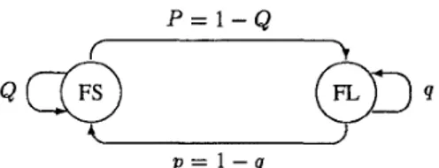
A p = l - q

Figure 5: Gilbert loss model for the frame loss process.

(6) If w

<

n, set w := w

+

1, and go to step (4).

(7) For v = 0 , 1 , 2 , .

. . ,

n, compute

where p e t is the effective normalized tagged load given by (3), and is equal to the sum of all pi for i E SS U SL.

Note that, in step (4), we have a set of ]SI,

I

linear equations with

(SI,( unknowns, where IS0

1

is thenumberofstates inSD. That is, we have to solve the matrix equation

Ax

= y for column vector x, where A is an IS0

I

x /SI,

I

matrix. Although ISD

I

M

[SE

I

/2 is very large for realistic N and B,

A

is a sparse matrix, and hence, the solution for the unknowns is feasible. Yet the algorithm requires (n

+

1) (n

+

2)/2

-

1 such solutions, and the complexity is determined mainly by this step. Therefore, the frame size n for which the CLPD computation takes a reasonable time is limited for realistic N and B.

3.3

Frame

Loss

Process Characterization

Let a frame with more than h missing cells be defined to be lost. Then, observe that frame losses are also correlated in time due to the correlation between the adjacent cells of consecutive frames. This has to be incorporated into the analysis in order to obtain accurate results in the frame coded cases. For this purpose, we approximate the frame loss process by a two-state MC, i.e., by the Gilbert Loss Model (GLM) shown in Figure 5, where the states FS and FL stand for frame success and loss, respectively. The computation of the GLM parameters Q and q based on the extended 3-D MC model will be discussedin [16].

Similar to the CLPD, let {G(v, n’) : v = 0,1,2,.

. .

,

n’}, be the Frame Loss Pattem Distribution (FLPD), where G(v, n’) is the probability of v frame losses in a coding matrix of n’ frames. To compute the FLPD based on the GLM, let us also define

g f s ( v , w) and gfi(v, w), v = 0 , 1 , 2 , .

. .

,

w, as the conditional probabilities of losing v of next w frames given that the current frame is successful and lost, respectively. Then, similar to the CLPD computation, the FLPD can be computed by the following iterative algorithm:

(I) Initialcondition: gfd(O,O) = grl(0,O) = 1.

(2) Boundarycondition: gjs(v, w ) = gjl(v, w) = Oif v

>

w (3) Set w := 1.

For v = 0,1,2,

.

.

. ,

w, compute

gfs(v, w) = Q g f s ( v , - 1)

+

P g j l ( u - 1, w - 11, (14)

and

S f I ( ” , w) = pg.f.(w’, w

-

1)

+

99fI(W

-

1,w

-

1). (15) If w

<

n’, set w := w

+

1, and go to step (4).

For w = 0,1,2,

. . .

,

n’, compute

G(v, n’) = Pfsgfs(v, n’)

+

P f i g j l ( ” , n’) (16) where, similar to (l),

Pfs

and Pfl are given respectively by (17) (18)

Pfs

= P / ( P

+

PI,

Pfl

= P/(P

+

P ) . and

Observe that, given the GLM parameters Q and q, this algorithm is of negligible complexity as compared to that of Section 3.2 used for the CLPD computation. However, the computation of

Q and q requires an additional execution of the former algorithm (see [16]). Therefore, given N and B , the frame size n is the major quantity that is constrained so that the CLPD and FLPD computations are both feasible, whereas there is not any practical limit on the coding block size n’.

3.4 Performance Evaluation

Observe that the most natural decoding strategy for the two- level coding scheme is to recover lost cells within each frame as frames are being received, and to check columns independently for subsequent possible recoveries upon reception of the whole coding matrix. Since recoveries over columns may enable new recoveries over rows and vice versa, it is possible to achieve bet- ter performance than that offered by this single-truce decoding, and the optimal decoder is the one which traces the coding matrix successivelyover rows and columns until no more new recoveries are left. However, due to the high computational complexity of our analytical framework, we consider a much simpler decoding strategy for the frame coded cases. We assume that column decod- ing is performed in a constrained manner over successful frames only, instead of independent recoveries over columns. In other words, the successful cells of lost frames are ignored. Although this constraineddecoding weakens the code interleaving effect of frame coding, the results of Section 4 indicate that the associated frame coding gain can still be quite significant.

After this simplifying assumption, the cell and frame loss rates, abbreviated respectively as CLR and FLR, follow eas- ily for the uncoded and coded cases. For any normalized ag- gregate load p E (0,1], let {Fhhr(v, n ) : v =

o,

1,2,.

. . ,

n } be the CLPD computed with the effect of parity overhead taken into account as described in Section 3.1. Also let {Ghhr

(w,

a’) :

w

= o,I, 2,

. . .

,

n’} be the K P D computedsim- ilarly. Then, the FLR defined as the ratio of the expected number

of unrecoverable frame losses in a coding matrix to n’ is given by

u = h ’ + l

since up to h’ frame losses in a coding matrix of n’ frames can be recovered. On the other hand, the CLR defined similarly as the ratio of the expected number of unrecoverable cell losses in a coding matrix to nn‘ is given by

where

nr

E

[rift]

= vGhh’(v,n‘) (21)

v = h ’ + l

is the expected number of unrecoverable frame losses in a coding matrix, and

/ n \ - 1 n

\ v = h + l / v = h + l

(22) is the expected number of cell losses in a frame that is given to be lost.

When there is no frame coding, it can be shown that (19) and (20) reduce respectively to

n

and

v = h + l

In the particular case of no coding, it can also be shown that (24)

further reduces to

where p i = p / N is the normalized tagged load, as (2) implies.

4

Results and Discussion

In this section, we fix the number of sources as N = 16 to obtain a reasonable traffic mix, and study the effectiveness of the two-level coding scheme via the analytical framework of Section 3 for a buffer capacity of B = 100 cells. We assume that only the tagged traffic is coded, and recalling the extremely diverse characteristics of the sources with clustering coefficients

c = 1.2 and c = 1.9 illustrated in Figure 3, consider interference of various combinations of these generic sources, which we refer to as “random” and “bursty” sources throughout this section.

We consider the homogeneous traffic scenarios R16 and B16, where all of the 16 sources are either random or bursty, respec- tively, and evaluate the performances of cell-only, frame-only, and joint cell-and-frame coding techniques separately for these two scenarios under heavy traffic conditions. In particular, for the B 16 scenario, we choose the normalized aggregate load to be

p = 0.8, which yields a CLR in the order of lo-* for the no cod- ing case. For the R16 scenario, since the CLR appears to be well

6b.3.6

16Wn

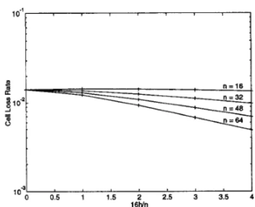
Figure 6: Effect of cell-only coding for the R16 scenario at p = 0.96, where n is the frame size in cells, and h is the number of parity cells in a frame.

below lo-’’ at p = 0.8 even when there is no coding, we choose a higher normalized aggregate load of p = 0.96. Although such high loads may not be typical for the long-term behavior of an ATh4 network, our steady state analysis thus gives emphasis to transient heavy traffic periods during which congestion is likelier to occur, and hence, FEC is functional. Furthermore, the gen- eral conclusions drawn are valid also for lower loads, as will be shown at the end of Section 4. We first study the effective- ness of cell-only coding for the homogeneous traffic scenarios R16 and B16. For both scenarios, we consider the frame sizes n E { 16,32,48,64}, and constrain the parity cells to constitute at most 25% of the total tagged traffic, i.e., h / n

5

0.25. For the R16 scenario, the CLRs computed at p = 0.96 are plotted in Figure 6. Observe that cell coding with n = 16 does not improve the CLR for any h

5

4. Referring to a frame with at least one lost cell as being corrupted, this is because a significant fraction of the corrupted 16-cell frames lose more than 4 cells. Since the most powerful erasure correcting code among those with the same rate is the one with the largest block length, the cell coding gain increases uniformly with n for any 0

<

h / n

5

0.25, and approximately 2.6 orders of magnitude reduction in the CLR is achieved when n = 64 and h = 16.

The cell-only coding results obtained at p = 0.8 for the B16 scenario are shown in Figure 7. Observe that Figures 6 and 7 exhibit similar trends in general. However, cell coding for the B16 scenario is not as effective as it is for the R16 scenario. This is obviously because the cell loss process is much burstier for the B16 scenario than it is for the R16 scenario. Better results can be achieved if larger frame sizes are considered, but frame coding with appropriate parameters should be expected to be far more effective.

The performance of frame coding depends not only on the parameters n’ and h’ but also on the frame size n. Too small an n may not provide sufficient code interleaving effect desired to overcome the burstiness of cell losses. On the other hand, given

n’ and h’, the larger n is, the larger the average decoding delay will be. Also since, when there is no cell coding, loss of even one cell results in the loss of the frame that it belongs to, the frame loss process is adversely affected by increasing n. Note that this

Figure 7: Effect of cell-only coding for the B16 scenario at p = 0.8, where n is the frame size in cells, and h is the number of

parity cells in a frame.

16hln’

Figure 8: Effect of frame-only coding with frame size n = 16 for the R16 scenario at p = 0.96, where n’ is the coding matrix size in frames, and h’ is the number of parity frames in a coding matrix.

effect is important for the constrained decoding strategy discussed in Section 3.4. As our preliminary results indicate that n = 16 is a reasonable choice in these respects for both traffic scenarios, we consider frame coding with n = 16 in the sequel.

For the R16 scenario, the results of frame-only coding with n’ E { 16,32,48,64} are shown in Figure 8, where p = 0.96 and h’/n’

5

0.25 again. Comparing these results with those of Figure 6, it is observed that frame-only coding with n’ = 16 improves the CLR slightly in contrast with the case for cell-only coding with n = 16. This indicates that although the sources are

highly random, cell losses are still bursty for the R16 scenario,

and hence, code interleaving provides an improvement. This is observed much more clearly for larger n’, and frame-only coding with n’ = 48 and h’ = 9, or with n’ = 64 and h’ = 8, outper- forms cell-only coding with n = 64 and h = 16. In particular, when n‘ = 64 and h’ = 16, the CLR is reduced by approximately 4.4 orders of magnitude as compared to the no coding case.

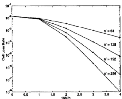
For the B16 scenario, the frame-only coding results obtained at p = 0.8 are shown in Figure 9. Due to the heavily bursty nature of cell losses, n‘

<

64 does not yield significant im-

Figure 9: Effect of frame-only coding with frame size n = 16 for the B16 scenario at p = 0.8, where n’ is the coding matrix size in frames, and h’ is the number of parity frames in a coding matrix.

provements. Therefore, we consider frame-only coding with

n’ E (64,128,192,256). Comparing Figures 7 and 9, observe that frame coding is much more effective than cell coding as expected. In particular, approximately 6 orders of magnitude reduction in the CLR is achieved when n’ = 256 and h’ = 64.

Note that these significant frame coding gains for both traffic scenarios are achieved despite the constrained decoding strategy. Much better results should be expected when we switch to the single-trace decoding which treats the columns of the coding ma- trix independently.

Also observe that the frame coding gain saturates with in- creasing h’/n‘ for the R16 scenario (see Figure 8). In fact, when

n’ = 16, there is a relative worsening for h’ = 4 as compared to h’ = 3. Referring to a coding matrix with at least one lost frame as being corrupted, this saturation indicates that a significant frac- tion of the corrupted coding matrices amve with no more than 0 . 2 5 ~ ~ ‘ lost frames. When n’

1

32, if h’/n’ is increased further from 0.25, the increase in the tagged load due to the parity over- head will start to dominate, and a relative worsening will occur as in the case of n’ = 16 and h‘ = 4. For this reason, we do not consider h‘

>

0.2%’.

Contrary to this behavior, the frame coding gain does not saturate within the range h’/n’

5

0.25 for the B16 scenario (see Figure 9). Even for n’ = 256, a significant fraction of the corrupted coding matrices lose more than 6.25% of their frames, and hence, frame coding with h’ = 0.0625n’ does not improve

the CLR for any n’ considered. As h ‘ / n ’ increases, it becomes more effective. The trend toward h’/n’ = 0.25 indicates that there is still a significant fraction of the corrupted coding matrices that lose more than 25% of their frames. However, we do not increase h’/n’ further from 0.25 since otherwise the resulting frame code will no longer be efficient.

For the case of joint coding, we choose n = 16 and n’ = 64 for the R16 scenario. The CLRs computed at p = 0.96 are shown in Figure 10, where the total number of parity cells in the coding matrix is constrained to be less than 0.3nn’. Observe that, although cell coding with n = 16 alone is not effective for any h

5

4, it provides a significant improvement when used together with frame coding. In particular, when n’ = 64 and h’ = 16,

t6h’In’ h

Figure 10: Effect of joint coding with frame size n = 16 and coding matrix. size n’ = 64 for the R16 scenario at p = 0.96, where h is the number of parity cells in a frame, and h’ is the

number of parity frames in a coding matrix.

0

16h’ln’ h

Figure 11: Effect of joint coding with frame size n = 16 and coding matrix size n’ = 256 for the B16 scenario at p = 0.8, where h is the number of parity cells in a frame, and h’ is the number of parity frames in a coding matrix.

even the simple single-parity cell coding with n = 16 reduces the CLR by approximately 2.3 orders of magnitude as compared to the frame coding alone. With the constrained decoding strategy in mind, this is because cell coding can improve the frame loss process characteristics, and in tum, increase the effectiveness of frame coding considerably.

For the B16 scenario, the joint coding results obtained at

p = 0.8 are shown in Figure 11, where n = 16 and n’ = 256. Similar to the case for the R16 scenario, cell coding increases the effectiveness of frame coding. However, the additional gain is not as significant as it is for the R16 scenario. Nevertheless, despite the heavily bursty nature of cell losses, cell coding with

n = 16 and h = 1 provides an additional gain of approximately 1.4 orders of magnitude as compared to frame-only coding with n’ = 256 and h’

=

64.

The results for the R16 and B16 scenarios are summarized in Table1,wherePP = 100(1-kk’/nn’)istheparitycellpercent- age, and G is the coding gain measured in orders of magnitude. Comparing the CLRs for the codes with P P x 25%, it is ob-

7 35

6b.3.8

Table 1: Summary of the results for the R16 and B16 scenarios respectively at p = 0.96 and p = 0.8, where n is the frame size in cells, h is the number of parity cells in a frame, n’ is the coding matrix size in frames, and h’ is the number of parity frames in a coding matrix.

Figure 12: Comparison of the codes with P P M 25% of Table 1 for the R16 scenario. The coding parameters are indicated in the [ ( n , h ) , (n‘, h,‘)] format, where h is the number of parity cells in a frame of n cells, and h‘ is the number of parity frames in a coding matrix of n’ frames. Continuous curves are the computational results, and discrete points are the simulation results.

served that, for the R16 scenario, the joint code outperforms both the cell-only and frame-only codes. For the B 16 scenario, on the other hand, the most effective code among those with P P M 25% is the frame-only code. Due to the heavily bursty nature of cell losses, the probability of having scattered cell losses over the cod- ing matrix is negligible. Therefore, for any P P given, it is better to arrange the whole parity overhead in the form of parity frames. Figures 12 and 13 compare the performances of the codes with P P M 25% of Table 1 respectively for the R16 and B16 traffic scenarios, where the CLR is plotted as a function of p for each code. By these comparisons, the superiority of the joint code for the R16 scenario, and that of the frame code for the B 16 scenario are validated for a wide range of p .

We have also simulated transmission of 10’ tagged cells for both scenarios, and the results are shown in comparison with the computational results in Figures 12 and 13. The almost perfect

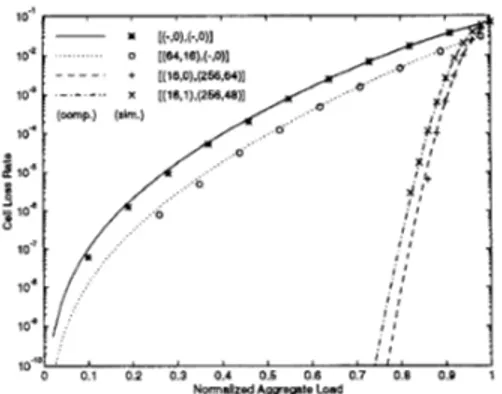
Figure 13: Comparison of the codes with P P G 25% of Table 1 for the B16 scenario. The coding parameters are indicated in the [ ( n , h ) , (n’, h’)] format, where h is the number of parity cells in a frame of n cells, and h’ is the number of parity frames in a coding matrix of n’ frames. Continuous curves are the computational results, and discrete points are the simulation results.

matches in the uncoded and cell-only coded cases for the B16 scenario and in the uncoded case for the R16 scenario are because we have not made any simplifying assumptions in these cases, and indicate the accuracy of the analytical model in capturing the bursty nature of cell losses. The slight deviation in the cell-only coded case for the R16 scenario should be attributed to the fact that the smaller the CLR is, the lower the confidenceof a fixed-length simulation becomes.

Observe that the GLM approximation to the frame loss process summarizes the cell loss behavior roughly from frame to frame. It claims that the loss and success of a frame both depend merely on the loss and success of the previous frame. The extent to which this claim holds is determined basically by the burstiness of cell losses and the frame size. Obviously, the larger the frame size is, the less relevant the information about more than just one preceding frame is, and consequently, the more accurate the GLM approximation becomes. The surprisingly perfect match in the frame coded cases for the B16 scenario indicates that the GLM approximation works quite well in this respect with n = 16 for bursty traffic. Unfortunately, the simulation results for the R16 scenario reveal that the analysis is underestimating the CLR by approximately an order of magnitude in the frame coded cases for random traffic. To figure out the reason of this difference, we ran simulations to find the consecutive frame loss and suc- cess length distributions for both traffic scenarios. For the R16 scenario, although the consecutive frame loss behavior is found

to be well-approximated by a simple geometric distribution as in

the case for the B16 scenario, thus justifying the sufficiency of one frame loss state in the GLM, the likelihood of the success of a frame increases abruptly after the number of consecutively preceding successful frames exceeds a certain threshold. This in- dicates that, for the R16 scenario, the consecutivesuccessof a few 16-cell frames may correspond to an occasional success period in the close neighborhood of frame loss, and hence, the past infor- mation of success of just one preceding frame is not sufficient to accurately determine what will happen next. As we switch

to the B16 scenario, the cell loss process gets burstier, and the success of only one preceding 16-cell frame carry almost all the relevant past information. Consequently, one frame success state in the GLM suffices. Although, in light of these observations, the analysis can be improved by exploiting a more complicated frame loss process model with more than one success states, additional computational complexity will be very high.

5 Summary and Conclusions

We have considered a two-level forward error correction scheme for lost cell recovery in ATM networks. The scheme is basedon transmitting parity cells, which are generated by using optimal, maximum distance separable erasure correcting codes, along with the information-bearing ones, and composed of two types of coding: (i) cell coding (appending h parity cells to every group of

k

consecutive information-bearing cells to form n-cell frames); and, (ii) frame coding (appending h’ parity frames to ev- ery group of

k‘

consecutive information-bearing frames to form n’-frame coding blocks).

Several papers have previously proposed and studied the per- formances of cell and frame coding techniques separately, via simulations andor analytical methods [31-[5], [8]-[11]. This pa- per differs from the previous work mainly in that it has combined the two individual coding techniques in order to achieve efficient recovery of burst as well as random cell losses, and carried out a comparative performance analysis of the cell-only, frame-only, and joint cell-and-frame coding techniques separately for random and bursty traffic streams under various interfering traffic condi- tions.

To analyze the coding performance for a delay-sensitive vir- tual channel traffic traversing a single node, we have developed a new, discrete-time analytical framework which allows accurate quantification of the cell and frame loss rates. The crucial aspect of this framework is explicit incorporation of the burstiness of traffic streams into a Markov chain model for the output buffer occupancy at the node. Based on this model which character- izes the cell loss process precisely, we have provided iterative algorithms to compute the loss rates for the uncoded and coded cases.

The performance results obtained indicate that although trans- mitting parity cells increases the network load, an appropriately chosen one of the three coding techniques can improve the end- to-end reliability significantly over a wide range of network load without requiring retransmissions. Since the coding performance is not much sensitive to the interfering traffic characteristics, the determination of the coding technique to be used can be based merely on the nature of the traffic stream for which forward error correction is desired. In particular, for a stream of cells dispersed evenly over time, although joint coding outperforms both of the individual coding techniques, cell coding alone may suffice since it yields substantial reductions (by several orders of magnitude) in the cell loss rate with smaller average decoding delay. For a bursty cell stream, on the other hand, cell coding is not effective at all simply because not only the rate but also the burstiness of cell losses increases as the traffic gets burstier. In this case,

code interleaving is required, and frame coding which serves this purpose is quite effective.

Joint coding combines the early and burst cell loss recovery capabilities of the cell and frame coding techniques, and provides fairly good performance improvement regardless of the traffic characteristics. Therefore, it is preferable especially when the nature of the traffic stream is not known a priori, or subject to change in time. It should be preferred also when forward error correction is to be performed for a virtual path connection onto which several individual traffic streams of different characteristics are multiplexed.

References

V.K. Bhqava, D. Haccoun, R. Matyas, and P.P. Nuspl, Digital Communications by Satellite: Modulation, Multiple Access and Coding. New York: John Wiley&Sons, Inc., 1981.

N.F. Maxemchuk, “Dispersity routing,” Proc. ICC’75, pp. 41 .lo- 41.13, San Francisco, CA, June 1975.

N. Shacham, “Packet recovery and error correction in high-speed wide-area networks,” Proc. MILCOM’89, pp. 29.5.1-29.5.7, May 1989.

N. Shachani and P. McKenney, “Packet recovery in high-speed net- works using coding and buffer management,” Proc. INFOCOM’90,

pp. 124-131, San Francisco, CA, June 1990.

T. Kitami and I. Tokizawa, “Cell loss compensation schemes em- ploying error correction coding for asynchronous broadband ISDN,”

Proc. INFOCOM’90, pp. 116-123, San Francisco, CA, June 1990. A.J. McAuley, “Reliable broadband communications using a burst erasure correcting code,” Proc. ACM SIGCOMM ’90, pp. 287-306, Philadelphia, PA, September 1990.

E. Ayanoglu, R.D. Gitlin, P.K. Johri, and W.S. Lai, “Protocols for errorfloss recovery in broadband ISDN,” Proc. 7-th Int’l. Telefrafic Congr: Sem., Morristown, NJ, October 1990.

L. Zhang and K.W. Sarkies, “Modeling of a virtual path and its applications for forward error recovery coding schemes in ATM networks,” Proc. SICON’91, pp. 259-264, Singapore, September 1991.

H. Ohta and T. Kitami, “A cell loss recovery method using FEC in ATMnetworks,”IEEEJSAC,vol.9, no.9,pp. 1471-1483,December 1991.

L. Zhang, “Statistics of cell loss and its application for forward error recovery in ATM networks,” Proc. ICC’92, pp. 325.3.1-325.3.5, Chicago, IL, June 1992.

E.W. Biersack, “Performance evaluation of forward error correc- tion in ATM networks,” Proc. ACM SIGCOMM’92, pp. 248-257, Baltimore, MD, August 1992.

N.C. Oguz and E. Ayanoglu, “A simulation study of two-level for- ward error correction for lost packet recovery in B-ISDN/ATM,”

Proc. ICC’93, pp. 1843-1846, Geneva, Switzerland, May 1993. W. Stallings, ISDN and Broadband ISDN. New York: Macmillian Publishing Company, 1992.

R.E. Blahut, Theory and Practice of Error Control Coding. Mas- sachusetts: Addison-Wesley Publishing Company, Inc., 1983.

I. Cidon, A. Khamisy, and M. Sidi, “Analysis of packet loss

processes in high-speed networks,” ZEEE Trans. Inform. Theory,

vol. 39, no. 1 , pp. 98-108, January 1993.

N. C. Oguz, Ph. D. Thesis, Bilkent University, Ankara, Turkey.

6b.3.10