PID controller design for first order unstable time delay systems

PID CONTROLLER DESIGN FOR FIRST ORDER

UNSTABLE TIME DELAY SYSTEMS

a thesis

submitted to the department of electrical and

electronics engineering

and the institute of engineering and sciences

of bilkent university

in partial fulfillment of the requirements

for the degree of

master of science

By

G¨ul Ezgi Arslan

July 2009

I certify that I have read this thesis and that in my opinion it is fully adequate, in scope and in quality, as a thesis for the degree of Master of Science.

Prof. Dr. Hitay ¨Ozbay(Supervisor)

I certify that I have read this thesis and that in my opinion it is fully adequate, in scope and in quality, as a thesis for the degree of Master of Science.

Prof. Dr. ¨Omer Morg¨ul

I certify that I have read this thesis and that in my opinion it is fully adequate, in scope and in quality, as a thesis for the degree of Master of Science.

Ass. Prof. Dr. Ulu¸c Saranlı

Approved for the Institute of Engineering and Sciences:

Prof. Dr. Mehmet Baray

ABSTRACT

PID CONTROLLER DESIGN FOR FIRST ORDER

UNSTABLE TIME DELAY SYSTEMS

G¨ul Ezgi Arslan

M.S. in Electrical and Electronics Engineering

Supervisor: Prof. Dr. Hitay ¨

Ozbay

July 2009

In this thesis, problem of designing P, PI and PD-like controllers for switched first order unstable systems with time delay is studied. For each type of con-troller, the problem is solved in two steps. First, the set of stabilizing controllers for the class of plants considered is determined using different approaches. Then, an appropriate controller inside this set is chosen such that the feedback systems satisfies a desired property, which is for example gain and phase margin max-imization or the dwell time minmax-imization. In the first part, we focus on PI controllers and tune the PI controller parameters in order to maximize the gain and phase margins. The observations in this part show that a P controller is adequate to maximize gain and phase margins. Then, we move on to the prob-lem of tuning P, PI and PD-like (first order stable) controller parameters such that the switched feedback system is stabilized and the dwell time (minimum required time between consequent switchings to ensure stability) is minimized. For this purpose, a dwell-time based stability condition of [39] is used for the class of switched time delay systems. We show that a proportional controller can be found with this method, but a PI controller is not feasible. Finally, we focus

time delays. The proposed method finds the values of PD-like (first order stable) controller parameters which minimize an upper bound of the dwell time. The conservatism analysis of this method is done by time domain simulations. The results show that the calculated upper bound for the dwell time is close to the lower bound of the dwell time observed by simulations. In addition, we compare the obtained PD-like controller results with some alternative PD and first order controller design techniques proposed in the literature.

Keywords: Stability Analysis, Switched Systems, Time Delay, PID Control,

¨

OZET

B˙IR˙INC˙I DERECEDEN ZAMAN GEC˙IKMEL˙I VE KARARSIZ

S˙ISTEMLER ˙IC

¸ ˙IN PID DENETLEY˙IC˙I TASARIMI

G¨ul Ezgi Arslan

Elektrik ve Elektronik M¨uhendisli¯gi B¨ol¨um¨u Y¨uksek Lisans

Tez Y¨oneticisi: Prof. Dr. Hitay ¨

Ozbay

Temmuz 2009

Bu tezin kapsamında birinci dereceden anahtarlamalı, kararsız ve zaman gecikmeli sistemler i¸cin orantısal denetleyici (P), orantısal-t¨umlevsel denetleyici (PI) ve orantısal-t¨urevsel denetleyici benzeri (PD-like) denetleyici tasarımı prob-lemlerinden bahsedilmi¸stir. Bu tip denetleyiciler i¸cin problemi iki adımda ¸c¨oz¨uyoruz. ˙Ilkinde, bahsedilen sistem grubu i¸cin farklı yakla¸sımlar kullanarak geribesleme sisteminin kararlılı˘gını sa˘glayacak denetleyici k¨umesi bulunmu¸stur. Daha sonra, bu k¨umenin i¸cerisinden istenen ¨ozellikleri sa˘glayan uygun denetleyici se¸cilmi¸stir.

Tezin ilk kısmında kazan¸c ve faz paylarını maksimize edecek PI denetleyici tasarımı ¨uzerine yo˘gunla¸stık. Kazan¸c ve faz paylarını azami yapmak i¸cin P denetleyicinin yeterli oldu˘gunu g¨ozlemledik. Daha sonra anahtarlamalı ve za-man gecikmeli sistemler i¸cin denetleyici tasarımı konusuna ge¸ctik. Bunun i¸cin, [39]’de verilen oturma zamanı hesabını temel alan kararlılık ko¸sulları kullanıldı. Bu y¨ontem kullanılarak, uygun bir P ve PD benzeri denetleyici bulunabildi,

an-¨uzerinde yo˘gunla¸stık. ¨Onerilen y¨ontemle PD benzeri (birinci dereceden kararlı) denetleyici parametreleri bulundu, bu denetleyici tipi i¸cin zamanda benzetim yapılarak korunumluluk analizi yapıldı ve elde edilen PD benzeri denetleyiciler literat¨urde bulunan alternatif tasarım teknikleri ile kar¸sıla¸stırıldı. Sonu¸clar hesa-planan oturma zamanı ¨ust sınırının benzetimler yardımıyla bulunan alt sınıra olduk¸ca yakın oldu˘gunu g¨osteriyor.

Anahtar Kelimeler: Kararlılık Analizi, Anahtarlamalı Sistemler, Zaman Gecikmesi, PID Denetleyici, Oturma Zamanı, Kazan¸c Payı, Faz Payı

ACKNOWLEDGMENTS

I would like to express my deep gratitude to my supervisor Prof. Dr. Hitay ¨

Ozbay for his unlimited support and guidance.

I would like to thank Prof. Dr. ¨Omer Morg¨ul and Assist. Prof. Ulu¸c Saranlı for reading and commenting on this thesis and for being on my thesis committee.

I would also like to thank my dear friends Sevin¸c Figen ¨Oktem, Esra Abacı and G¨okhan Bora Esmer for their unlimited support.

I would like to thank Bilkent University EE Department and T ¨UB˙ITAK for their financal support.

Last but not the least, I would like to thank my husband and my parents for their support and endless love through my life.

Contents

1 Introduction 1

2 PI Controller Design Based on Gain and Phase Margin

Maxi-mization and a Cost Function MiniMaxi-mization 8

2.1 Gain Margin Maximization . . . 11

2.2 Phase Margin Maximization . . . 13

2.3 Gain and Phase Margin Optimization . . . 18

2.4 Cost Function Minimization . . . 22

2.5 Transient Response Optimization . . . 27

3 P and PI Controller Design for A Switched System Using the LMI-based Stability Test Given in [39] 32 3.1 Proportional Control . . . 34

3.2 Proportional-Integral Control . . . 40

4 PD-like Controller Design for A Switched System Using the

4.1 Conservatism Analysis and Simulations . . . 47

4.2 Comparison of the Results with Alternative Design Methods . . . 53

5 Conclusions 65 APPENDIX 68 A The Matlab Codes 68 A.1 PI Control for Gain and Phase Margin Maximization . . . 68

A.2 P Control for Dwell Time Minization . . . 73

A.3 PD-like Control for Dwell Time Minization . . . 75

A.3.1 Conservatism Analysis . . . 78

List of Figures

1.1 Typical Switched Feedback System . . . 4

2.1 The Gain Margin versus τ . . . 13

2.2 K versus τ . . . 14

2.3 Kτ versus τ . . . 15

2.4 φ(ω) versus frequency ω . . . 16

2.5 Phase margin φm versus τ . . . 17

2.6 Gain crossover frequency ωg versus τ . . . 18

2.7 K versus τ . . . 19

2.8 Kτ versus τ . . . 20

2.9 A typical phase φ(ω) versus frequency ω graph . . . 21

2.10 Step response of the obtained system . . . 22

2.11 The Nyquist Plot of the Feedback System for τ = 1 . . . 23

2.12 The Nyquist Plot of the Feedback System for τ = 100 . . . 24

2.14 α versus τ Graph . . . 26

2.15 Cost function J versus τ Graph . . . 27

2.16 Step response of the system when c = 1 . . . 28

2.17 The Root Locus of the Closed-Loop System . . . 29

2.18 Settling time versus τ . . . 30

2.19 The σ−1 s of the system . . . 31

3.1 A Typical Parabola of P (α) = aα2_{+ bα + c with a > 0 . . . 37}

3.2 The minimum dwell time τ with changing time delay h . . . 40

4.1 The parameters of the controller versus delay . . . 48

4.2 The parameters of the controller versus delay . . . 49

4.3 The minimum dwell time versus delay . . . 50

4.4 Dwell time from simulations . . . 51

4.5 Dwell time from simulations when Pade order=8 . . . 52

4.6 Dwell time versus Pade order . . . 53

4.7 Stability domains in (Kp− Kd) plane with various delays . . . 55

4.8 A typical stabilizing region in (Kp− Kd) plane . . . 56

4.9 The stabilizing region of (α2, α3) when α1 = 1 . . . 60

4.10 The dwell time τ versus time delay h . . . 62

List of Tables

2.1 Maximum Gain Margin and Phase Margin Results For Corre-sponding τ values . . . 20

2.2 Maximum Gain Margin GM and Phase Margin φm Results For Corresponding c . . . 25

3.1 The minimum dwell time τ with changing time delay h . . . 39

4.1 The minimum dwell time τ versus delay . . . 47

4.2 The minimum and maximum bounds of the controller parameters

Kp and Kd for h = 0.1 . . . 61

4.3 The minimum dwell time τ of different design methods with time delay h = 0.1 . . . 61

Chapter 1

Introduction

PID controllers offer the simplest and yet most efficient solution to many real world control problems. Therefore, they are the most widely used controller structures in the industry, [1]. The user has to tune three controller parameters in this setting. With the advances in the technology, automatic control area can now offer a wide range of controller structures. However, PID controllers are the most dominating. More than 90% of the controller loops used in the industry consists of PID controllers, [3]. PID controllers are used in various applications such as: process control, motor drives, magnetic and optic memories, automo-tive, flight control, instrumentation, etc. According to [38], PD control is most frequently used in robot position and force control because of its robustness to time delay and in addition, 98% of control loops in the pulp and paper industries are controlled by PI controllers, [23]. Another strength of the PID controller is that it deals with some practical issues such as actuator saturation and integrator windup. The PID controllers of interest are in the following form:

C(s) = Kp+ Ki s + Kds τds + 1 (1.1) where Kp is the proportional constant, Ki is the integral constant, Kd is the derivative constant and τd > 0 is a small time constant. The derivative part of

Traditionally, the derivative part of a standard PID controller is filtered with a low-pass filter to prevent the high frequency gain of the controller growing too much (see [18]). The filter has not been regarded as a part of the design but added afterwards with the filter constant adjusted appropriately for the system to meet the specifications and small enough not to influence mid-frequency com-ponents. Also, note that when τdis an arbitrary positive number, (1.1) represents a stable controller structure. Such controllers are also have practical significant importance in the framework of low order strongly stabilizing controller design for unstable time delay systems, see e.g. [11] and [24].

In this thesis, we focus on PID (or stable) controller design for switched first order unstable systems with time delay. The transfer function of a first order time delayed unstable plant is as follows:

P (s) = e

−hs

s − a (1.2)

where h > 0 is the time delay and a > 0 is the right half plane pole. A typical example of a first order unstable system with time delay is an aircraft model, [7]. The transfer function of the form (1.2) forms a distributed model of the aircraft for the purpose of controlling the longitudinal dynamics of an aircraft in the short time period. That means, only two parameters h and a model an infinite dimensional dynamics. In addition, the high frequency dynamics due to elasticity, actuators, sensors, computer and zero order hold contribute the effective time delay. Another example of such a system is the batch chemical reactor which has a strong nonlinearity due to heat generation term in the energy balance, see [21]. It is well known that we can effectively approximate a higher order transfer function with a first order time delayed transfer function. Thus, a wide range of plant structures can be handled by investigating the first order unstable plant with time delay.

It is difficult to control a plant if the product of the time delay and the right half plane (RHP) pole is large. A good example for demonstrating this fact is the

NASA X-29 forward-swept-wing aircraft, see [33]. The product of effective time delay and unstable pole was 0.37, see [21]. Although X-29 was built to illustrate the aerodynamic performance improvements, after lots of test, it was discovered that the vehicle was too unstable to control with the given hardware. Therefore, the product of effective time delay and unstable pole is a prominent parameter in terms of ‘difficulty of control ’. Moreover, [5] and [36] reported that a well tuned P or PI controller could stabilize a first order unstable plant with time delay if and only if the product of effective time delay and unstable pole ah < 1 is satisfied.

Over the last four decades, various methods were developed for setting the parameters of P, PI, PD and PID controllers. Some of these methods are mod-ifications of the frequency response method introduced by Ziegler and Nichols, see [40], [12] and [4]. Some effort has been made to obtain an analytical formula which is only possible through rough approximations, see [13] and [17]. [37] de-veloped tuning formulas based on minimization of integral performance criteria, [26] developed a method for design of controllers based on model matching in frequency domain, [27] proposed explicit tuning rules based on IMC design and [5] and [13] proposed tuning rules based on gain and phase margin specifications. See [23] to find an excellent collection of these tuning rules. However, very few of them investigated the set of all stabilizing controllers, see [31], [29] and [30]. As a part of this thesis, we investigated the parameter space which ensures closed-loop stability with PID controllers. The solution to the PID stabilization problem is based on determining appropriate intervals for proportional, integral, derivative and time constant given in (1.1) where the obtained PID controller stabilizes the feedback system. The method for finding this parameter space is as following:

• First an admissible range for proportional constant is found for which a

• For a fixed proportional constant value in this range, the set of stabilizing

integral and derivative constant is found. It is either a trapezoid, a triangle or a quadrilateral.

• After determining the parameter space for proportional, integral and

derivative constants, an admissible range for time constant is found to ensure stability.

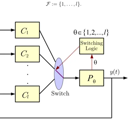
As far as switched systems are concerned, we consider the switched feedback system shown in Fig. 1.1, where θ is an arbitrary piecewise switching signal taking values on the set

F := {1, . . . , l}.

Figure 1.1: Typical Switched Feedback System

In this study, we assume that between switching time instants the plant is one of the elements of the following known set.

At each switching instant, the switching signal θ selects an index θ ∈ F, so a plant is selected from P. Each Pθ ∈ P is a first order unstable system with time delay and can be expressed in the following form:

Pθ(s) =

e−hθs

s − aθ

. (1.3)

where hθ is the time delay and aθ is the right half plane pole. As the plant switches according to the switching logic θ, controller has to switch in order to preserve stability. The controllers Cθ are proportional integral derivative (PID) controllers in the form:

Cθ(s) = Kpθ + Kiθ s + Kdθs τdθs + 1 (1.4) where Kpθ is the proportional constant, Kiθ is the integral constant, Kdθ is the derivative constant and τdθ > 0 is a small time constant. A state-space realization of the closed loop dynamics can be written as follows:

Σθ :    ˙x(t) = Aθx(t) + ¯Aθx(t − hθ) y(t) = Cθx(t) (1.5)

The triplet Σθ := (Aθ, ¯Aθ, hθ) is introduced to describe the θth candidate system of (1.5). Thus, ∀t ≥ 0 we have

Σt∈ A := {Σθ : θ ∈ F} where A is the family of candidate systems of (1.5).

The switching signal θ causes an arbitrary selection between candidate sys-tems and the selection of the switching signal for control purposes is out of the scope of this thesis. In other words, we deal with the system under arbitrary switchings in both the plant and the controller parameters, which are determined

The feedback system shown in Fig. 1.1, runs with the initial conditions which means the reference input is zero. Since each candidate plant is stabilized with a corresponding controller, the switched system will preserve its stability if the candidate plant-controller pairs are running for a long enough time interval. In other words, if the switching intervals are sufficiently long, the overall switched system will be stable. On the other hand, frequent switching may cause insta-bility, see e.g. [10], [22] and [34]. The minimum time needed between switching instants to maintain stability is called dwell time. An LMI-based stability con-dition is recently derived in [39], which also gives a dwell time expression. Using the derived LMI-based stability test, the set of stabilizing PID controllers for switched first order unstable plants is searched.

Our contributions can be summarized as follows:

• We investigate different PI controller design methods in literature and

de-velop a method based on gain and phase margin maximization and a cost function minimization for first order unstable time delayed plants given in (1.2). For the beginning, we deal with some controller design criteria for non-switched plants, including the gain margin and the phase margin optimization and a cost function minimization which is defined as a linear combination of the weighted sensitivity function and the vector margin.

• Then, we find a stabilizing parameter space for P and PI controllers and

develop a method using these parameter spaces for switched first order unstable plants with time delay using the LMI-based stability test derived in [39].

• Likewise, PD-like controller design approach is developed for the same class

of plants using the LMI-based stability test given in [39]. The conservative-ness of this method is tested using time domain simulations and the results of this methods are compared with some PID controller design methods mentioned above.

In Chapter 2, we provide the developed PI controller design method based on gain and phase margin maximization and a cost function minimization. Chap-ter 3 addresses P and PI controller design method we propose for switched first order unstable plants with time delay. In Chapter 4, the results of the PD-like controller design method for the same class of plants are given; the conservative-ness analysis of the results are done and comparisons of the proposed approach with the existing methods are made. We give the concluding remarks in Chap-ter 5.

Chapter 2

PI Controller Design Based on

Gain and Phase Margin

Maximization and a Cost

Function Minimization

For the plant of the form (1.2) and the PI controller of the form (1.1) where the derivative gain of the controller Kd = 0, the open-loop transfer function of the system is given by,

G(s) = C(s)P (s) = (Kps + Ki)e

−hs

s(s − a) (2.1)

which can be rewritten as;

G(s) = K(1 + τ ˆs)e −ˆhˆs ˆ s(ˆs − 1) (2.2) where K = Ki a2 , τ = a Kp Ki, ˆh = ha and ˆs = s

a. Therefore, in the rest of the chapter, we consider the generic form of the open-loop transfer function,

G(s) = K(1 + τ s)e

−hs

We think of

C(s) = K1 + τ s

s (2.4)

is the generic PI control and

P (s) = e

−hs

s − 1 (2.5)

is the generic plant.

In this chapter, our aim is to design the controller parameters K and τ such that for a given plant of the form (2.5).

• The gain and phase margin are maximized separately. • Gain and phase margin are optimized in a blended fashion.

• A cost function obtained from H∞ robust performance problem is mini-mized.

The phase margin, denoted by φm, is defined as;

|G(jωg)| = 1 (2.6)

φm = ∠G(jωg) + π (2.7)

where ωg is called the gain crossover frequency. The magnitude of G(jω) is a non-increasing function because G(jω) has one pole at ω = 0 and one real pole and zero, hence there exists a unique gain crossover frequency.

In order to ensure the feedback system stability, 1 + G(jω) has to encircle −1 once in the counterclockwise direction from the Nyquist encirclement principle. That means G(jω) have to intersect the negative real axis at least twice. This condition is satisfied if and only if

|G(jωp1)| > 1 > |G(jωp2)| (2.8)

where ωp is called the phase crossover frequency and ωp1 < ωp2 are the smallest

solutions of G(jω) = −π. The gain margin denoted by GM is defined as follows.

where σ1 = |G(jωp1)| and σ2 = |G(jωp2)|. Note that, this definition is different

from the classical gain margin definition (for example see [13])

GM = 1

σ2

.

Our definition is the same as the gain margin definitions in [20] and [9]. This def-inition is more appropriate for unstable systems in terms of robustness analysis, see [20].

In addition, the cost function obtained from robust performance problem, denoted by J, is defined as;

J = (cβ + eα)−1 (2.10)

where 0.01 ≤ c ≤ 40 is a coefficient to be adjusted, S denotes the sensitivity function given as follows,

S(s) = 1

1 + C(s)P (s) (2.11)

α is a robust performance measure defined as follows which is the infinite norm

of a weighted sensitivity function,

1

α = ||W (s)S(s)||∞ (2.12)

and β is called vector margin as defined in (2.13), which is the distance of G(jω) from −1.

1

β = kSk∞ (2.13)

The desired controller parameters should be chosen to satisfy robust stabil-ity and performance conditions. The necessary condition to satisfy the robust stability is to design a controller that stabilizes the nominal feedback system as

well as all the possible plants with additive uncertainty bounded by W (s). The vector margin β is a parameter related with the robust stability. For a robustly stable system, the controller should be designed to restrict the tracking error energy to satisfy robust performance criteria. Due to the robust performance constraint, the weight function is chosen as W (s) = 1

s in order to obtain a better tracking of step-like reference signals. Hence, α is a parameter related with the robust performance condition.

It is difficult to solve the above optimization problem analytically, hence we concentrate on numerical solutions.

2.1

Gain Margin Maximization

For a given plant (1.2), K and τ parameters in (2.3) are chosen such that the gain margin is maximized. The magnitude and phase expressions of the open-loop transfer function G(s), as shown below, are required to find the gain margin.

|G(jω)| = K ω r 1 + τ2_ω2 1 + ω2 (2.14) ∠G(jω) = −3π 2 + tan −1_{(τ ω) + tan}−1_{(ω) − hω (2.15)}

Proposition 1. For each fixed h > 0 and τ > 0, the optimal K maximizing GM

defined in (2.9) is: K = Ã 1 ωp1ωp2 s (1 + τ2_ω2 p1)(1 + τ 2_ω2 p2) (1 + ω2 p1)(1 + ω 2 p2) !−1 2 . (2.16)

Proof. Let ωp1 and ωp2 be the two smallest phase crossover frequencies satisfying

G(jωp) = −π. By substituting (2.14) into σ1 and σ2, we obtain the following

equations. σ1 = |G(jωp1)| = K ωp1 s 1 + τ2_ω2 p1 1 + ω2 p1 σ2 = |G(jωp2)| = K ωp2 s 1 + τ2_ω2 p2 1 + ω2 p2 Then define; a = 1 ωp1 s 1 + τ2_ω2 p1 1 + ω2 p1 (2.17) b = 1 ωp2 s 1 + τ2_ω2 p2 1 + ω2 p2 (2.18)

When a and b variables defined above are substituted into (2.8), we obtain

Ka > 1 > Kb. This inequality can be rewritten as follows.

1

b > K >

1

a (2.19)

The optimal K value satisfying (2.19) maximizing the gain margin defined in (2.9) is K = _√1

ab. If we substitute the a and b variables defined in (2.17) and (2.18), we obtain the optimal gain K as given in (2.16).

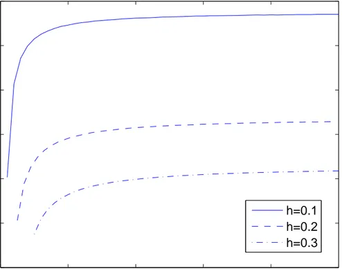
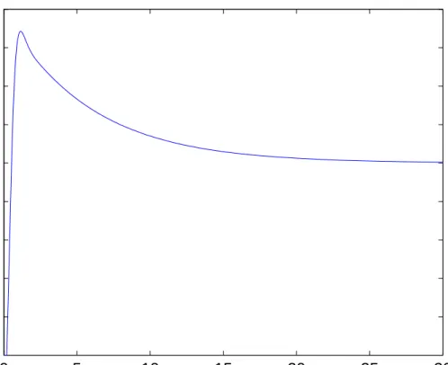
For the generic plant, for each fixed τ under the above choice of K, the variation of GM is as shown in Figure 2.1. As illustrated in the Figures 2.1, 2.2 and 2.3, higher τ value yields better gain margin and smaller K value. The controller can be considered as follows,

C(s) = Kτ +K

where Kτ is the proportional constant and K is the integral coefficient. From Figures 2.2 and 2.3, it could be seen that as τ → ∞, K → 0 and 0 < Kτ < ∞, which means the porportional constant is approaching to a constant finite value. Therefore, since the integral constant goes to 0, a proportional (P) controller is adequate to maximize the gain margin.

0 2 4 6 8 10 1 1.5 2 2.5 3 3.5 4

τ

GM

Figure 2.1: The Gain Margin versus τ

2.2

Phase Margin Maximization

Phase margin is a performance measure of the feedback system, which is related with the damping of the system, see [6]. In this section, we choose the controller parameters K and τ in (2.4) to maximize the phase margin, which is defined as follows.

1 2 3 4 5 6 7 8 9 0 2 4 6 8 10 12

τ

K

For each fixed τ , the maximum φ value and the corresponding gain crossover frequency, ωg, are found by evaluating (2.21) over a frequency range.

Proposition 2. For each fixed h > 0 and τ > 0, the optimal K maximizing the

phase margin can be expressed as:

K = ωg s 1 + ω2 g 1 + τ2_ω2 g (2.22)

where the gain crossover frequency, ωg, is obtained by setting the magnitude of

0 2 4 6 8 10 2 2.5 3 3.5 4 4.5 5

τ

K

τ

Proof. Let ωg be the gain crossover frequency satisfying

|G(jωg)| = 1. (2.23)

By substituting the magnitude of G(jω) given in (2.14) into (2.23), we obtain the following equality.

K ωg s 1 + τ2_ω2 g 1 + ω2 g = 1 (2.24)

Hence, the optimal K expression given in 2.22 for each fixed τ is derived from (2.24).

For the generic plant, the graph of

is shown in Fig. 2.4 for changing τ values. As we can see, φ(ω) has a maximum point for each τ value. We should adjust ωg such that

ωg = arg max(φ(ω)) (2.26)

The resulting phase margin φm versus τ and time delay h are illustrated in Fig. 2.5. 0 1 2 3 4 5 6 7 8 9 10 −5 −4.5 −4 −3.5 −3 −2.5 −2 φ ( ω ) ω h=0.2 τ is increasing from 0.1 to 103

Figure 2.4: φ(ω) versus frequency ω

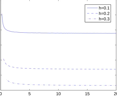
The variation of ωg versus τ with respect to different delay values is illustrated in Fig. 2.6 to show that as τ → ∞, the gain crossover frequency goes to a finite value.

In Figures 2.7 and 2.8, the graph of the proportional and integral constants versus τ are illustrated respectively with respect to time delay. As shown these

0 2 4 6 8 10 0 10 20 30 40 50 60

τ

φ

Figure 2.5: Phase margin φm versus τ

figures, higher τ value yields higher phase margin and smaller K. For the con-troller structure shown in (2.4), the same situation as the gain margin maxi-mization problem occurs. As τ → ∞, a higher phase margin is obtained with

K → 0 and Kτ approaches to a finite value. That means a P controller is

adequate to obtain the maximum phase margin from a stable feedback system. Same observations are made in [14]. In addition, as we know, phase margin has to be positive to ensure the stability of the feedback system. Therefore, for each

h > 0, we obtain a minimum τ > 0 value which makes the phase margin greater

100 101 102 103 1.5 2 2.5 3 3.5 4 4.5

τ

ω

(

τ

)

Figure 2.6: Gain crossover frequency ωg versus τ

2.3

Gain and Phase Margin Optimization

As we stated in the previous sections, gain margin and phase margin parameters are good measures of robustness. Therefore the aim in this section is to design a controller that satisfies both gain margin and phase margin criteria. The phase margin definition in (2.21) and the gain margin definition in (2.9) are used to maximize the gain margin and the phase margin in a blended fashion.

In order to optimize gain and phase margin in a blended fashion, the optimal

K value is chosen such that both gain and phase margin are maximized by

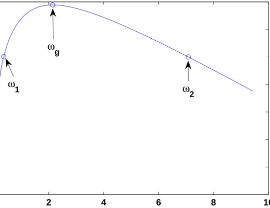
equat-ing the optimal K expression given in (2.16) and (2.22) for both gain and phase margin maximization problems. We can find the gain and the phase crossover frequencies in these expressions by evaluating the phase φ over a frequency range. Here, ω1and ω2 are the phase crossover frequencies where G(jω) = −π is satisfied

2 4 6 8 10 0 2 4 6 8 10 12 14

τ

K

and ωg is the gain crossover frequency where (2.23) is satisfied. A typical graph illustrating the phase crossover frequencies and the gain crossover frequency are as shown in Figure 2.9. By this way, the corresponding optimal K value is obtained.

Optimum gain and phase margin search explained above is accomplished over different τ values to choose corresponding τ that maximizes both parameters.

The maximum gain and phase margin values are indicated in Table 2.1 for each fixed τ and as τ → ∞, phase margin converges to 39.559 degrees and gain margin converges to 2.689.

Hence, the maximum gain and phase margins are obtained when τ goes to infinity and optimal K goes to zero which causes the integral action to disappear. In order not to get too small integral action gain, we may want to choose τ = 10

0 5 10 15 20 2 2.5 3 3.5 4 4.5 5 τ

K

τ

which yields K = 0.543, GM = 37.214 and φm = 2.645. The step response of this system is as shown in Figure 2.10.

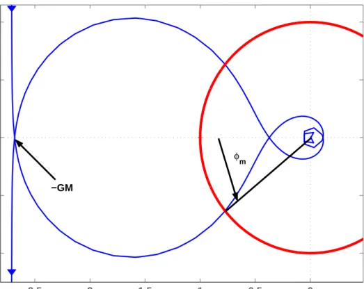
The Nyquist plots of the feedback system using the designed controller (under the choice of K defined above) for τ = 1 and τ = 100 are shown in Figures 2.11 and 2.12. Both of the Nyquist plots encircle -1 once in the counterclockwise direction, therefore feedback systems are stable. As illustrated in Figures 2.11 and 2.12, GM increases with increasing τ , because the magnitude of the negative

τ φm (in degrees) GM 1 18.680 2.196 5 34.913 2.600 10 37.214 2.645 50 39.103 2.683 100 39.333 2.683

Table 2.1: Maximum Gain Margin and Phase Margin Results For Corresponding

0 2 4 6 8 10 −280 −260 −240 −220 −200 −180 −160 −140

ω

φ

(

ω

)

ω

ω

ω

Figure 2.9: A typical phase φ(ω) versus frequency ω graph

real axis crossing to the left of −1 increases and the angle of the point which Nyquist plot intersects the unit circle increases with increasing τ , therefore phase margin increases.

The problem of optimization of gain and phase margins in a blended fashion can be solved with a P-type controller, because the parameters of the desired controller in (2.4) are τ → ∞ and K → 0 with Kτ finite. Therefore, as in the gain margin maximization and phase margin maximization problems, the feedback system is stable due to the proportional control but the tracking performance to a step-like reference signal is not good due to the lack of integral action.

0 5 10 15 20 25 30 0 0.2 0.4 0.6 0.8 1 1.2 1.4 1.6 1.8

time

Step Response

Figure 2.10: Step response of the obtained system

2.4

Cost Function Minimization

Solutions to gain and phase margin maximization problems yields a P-type con-troller, which is insufficient to obtain a good transient performance. Hence, by defining a cost function to minimize, we tried to put a bound on τ in (2.4) such that the designed controller is a PI-type controller and due to integral control, the feedback system provides a good tracking performance to step-like reference signals.

The cost function, denoted by J, is defined as follows,

J = (cβ + eα₎−1 _(2.27)

−3.5 −3 −2.5 −2 −1.5 −1 −0.5 0 0.5 −1.5 −1 −0.5 0 0.5 1 1.5 Nyquist Diagram Real Axis Imaginary Axis φ_m −GM

Figure 2.11: The Nyquist Plot of the Feedback System for τ = 1

1

β = kSk∞ (2.28)

1

α = ||W (s)S(s)||∞ (2.29)

Here, S is the sensitivity function defined in (2.11), β is vector margin which is defined as the distance of G(jω) from −1. For each fixed τ , the gain crossover frequency satisfying stability conditions (φm > 0) and optimal K in (2.22) are found by evaluating G(jω) over a frequency range. From these values, vector margin is evaluated by taking supremum over ω of the sensitivity function and α is found by taking supremum over ω of the weighting function W (s) = 1

s times the sensitivity function S.

−2.5 −2 −1.5 −1 −0.5 0 −1 −0.5 0 0.5 1 Nyquist Diagram Real Axis Imaginary Axis φm −GM

Figure 2.12: The Nyquist Plot of the Feedback System for τ = 100

For the generic plant, the variation of β and α over different τ values is as shown in Figures 2.13 and 2.14. As τ increases, vector margin increases and

α increases up to a point then decreases. In these figures, τ is greater than a

certain value for each time delay h > 0, because below these values the system becomes unstable.

Then, by combining α and β with c = 1 such that

J = (eα_{+ β)}−1_.

For the generic plant with h = 0.2, the variation of J versus τ is as shown in Fig. 2.15.

The optimum values of parameters satisfying the specified cost minimization problem is τ = 2.24, maximum gain margin GM = 2.48, maximum phase margin

0 2 4 6 8 10 0 0.1 0.2 0.3 0.4 0.5 0.6 0.7

τ

β

Figure 2.13: Vector Margin β versus τ Graph

obtained φm = 29.41 degrees and optimal K = 1.23. For the same system, the maximum gain and phase margins with changing c values are indicated in Table 2.2.

c φm (deg.) GM Optimal τ Optimal K

0.05 38.25 2.66 17.78 0.15 0.06 34.92 2.60 5.01 0.54 0.07 30.46 2.52 2.51 1.09 0.1 30.46 2.52 2.51 1.09 0.2 29.41 2.48 2.24 1.23 0.3 29.41 2.48 2.24 1.23 1 29.41 2.48 2.24 1.23

Table 2.2: Maximum Gain Margin GM and Phase Margin φm Results For Cor-responding c

The cost function does not have a minimum point for c > 40. The step response of this system with c = 1 is as shown in Figure 2.16. We can obtain the same results if we design a controller using the gain and phase margin results

0 2 4 6 8 10 0 0.5 1 1.5 2 2.5

τ

α

Figure 2.14: α versus τ Graph

obtained in Table 2.1 with the design methods given in [14]. If we compare our design with c = 1 and the design in [14] under 3 dB gain margin and 30 degrees phase margin specifications, we observe that the step responses of these designs which are illustrated in Figure 2.16 and the Figure 3 in [14] are similar. That means we obtained a step response with about 83% overshoot and 4 seconds of settling time in our design. Likewise, they obtained approximately 90% overshoot and 5 seconds of settling time. In addition, [14] showed that this design gives better results than the designs given in [5], [36] and [25].

If we compare the results obtained in Sections 2.3 and 2.4, the system designed in Section 2.3 has higher gain and phase margins, but the settling time of the system designed in Section 2.4 is lower which means this system has a better transient performance. In addition, the overshoot of the step response in Figure 2.16 is higher than the step response in Figure 2.10.

0 1 2 3 4 5 0 0.1 0.2 0.3 0.4 0.5 0.6 0.7 0.8 0.9

τ

J=(e

+

β

)

Figure 2.15: Cost function J versus τ Graph

2.5

Transient Response Optimization

Another method to improve the transient response is to adjust the dominant poles of the closed-loop system in order to obtain fast tracking of the reference signal. If the poles of the closed-loop system are denoted as pi’s, then we define a parameter related to the settling time as follows:

σ−1

s = (max_p

i

{Re{pi}})−1 (2.30)

We can minimize the σ−1

s parameter by placing the dominant poles far away from the imaginary axis. The aim in this section is to choose the controller parameters in order to place the dominant poles of the closed-loop system away from the imaginary axis.

0 5 10 15 20 25 30 0 0.2 0.4 0.6 0.8 1 1.2 1.4 1.6 1.8 2

time

Step Response

Figure 2.16: Step response of the system when c = 1

For the generic plant in (1.2) with h = 0.2, when we choose optimal K to maximize both gain and phase margins, the root locus of the closed-loop system is as shown in Fig. 2.17.

As we can see from 2.17, there are infinitely many complex conjugate poles due to the time delay and a real pole. For small τ values, the real pole is very close to origin and for increasing τ values, the real pole moves away from the origin. In contrast, the complex conjugate poles move towards the imaginary axis as τ is increasing. Initially, the real pole is the dominant pole and it moves away from the imaginary axis with the increasing τ . After a certain τ value, one of the complex conjugate poles become dominant which move toward the imaginary axis with the increasing τ . Therefore, the settling time decreases up to the certain τ value for each time delay and then increases, which is illustrated in Figure 2.18.

−25 −20 −15 −10 −5 0 −200 −150 −100 −50 0 50 100 150 200

Root Locus of the Closed−Loop System

Re(s)

Im(s)

Figure 2.17: The Root Locus of the Closed-Loop System

For h = 0.2, the minimum σ−1

s obtained is σs−1 = 0.477 with GM = 2.242,

φm = 20.29 degrees, τ = 1.1 and K = 2.589. The step response of this system is as shown in Figure 2.19.

0 1 2 3 4 5 0 0.5 1 1.5 2 2.5 3 3.5

τ

Inverse of the Real Part of the Largest LHP Pole

h=0.1 h=0.2 h=0.3

0 1 2 3 4 5 6 7 8 9 10 −0.5 0 0.5 1 1.5 2 2.5 Step Response Time (sec) Amplitude Figure 2.19: The σ−1 s of the system

Chapter 3

P and PI Controller Design for A

Switched System Using the

LMI-based Stability Test Given

in [39]

In this chapter, we first review some preliminaries from Linear Algebra.

Definition 1 (Principal Leading Minor). The kth _{order principal leading minor}

of an n × n matrix X , denoted by |Mk|, is the determinant of the first k rows

and columns of the matrix X .

Fact 1. A n × n matrix is negative definite if and only if ∀k ∈ {1, . . . , n} (−1)k_|M

k| > 0, where Mk’s are the principal leading minors of the

matrix.

Fact 2. Consider a second order polynomial with coefficients a, b and c. (P (x) =

ax2_{+ bx + c)}

• c

• −b

a is the sum of the roots P (x) = 0.

• If the discriminant of the polynomial (∆ = b2_{− 4ac) is negative and a > 0,}

then the polynomial is always positive for all x.

• If the discriminant of the polynomial (∆ = b2_{− 4ac) is positive and a > 0,}

then the polynomial is intersects the x-axis and becomes negative for some x.

The linear matrix inequality (LMI) based stability test derived in [39] for switched time delay systems is stated as follows.

Lemma 1. For each fixed time delay system of the form (1.5), the triplet defined

as,

Σ : (Aθ, ¯Aθ, hθ) ∈ Rn×n× Rn×n× R+ (3.1)

is asymptotically stable dependent of delay if the following inequality holds.

X :=   Λθ PθA¯θMθ MT θ A¯TθPθ −Rθ   < 0 (3.2) where Λθ = (Aθ+ ¯Aθ)TPθ+ Pθ(Aθ+ ¯Aθ) + τθpθ(αθ+ βθ)Pθ, Mθ = [Aθ A¯θ], Rθ = diag(αθPθ, βθPθ),

αθ > 0, βθ > 0, pθ > 1 are scalars and

Pθ ∈ Rn×n is a symmetric positive def inite matrix.

(3.3)

The variables αθ, βθ, pθ and Pθ are the decision variables of the inequality given in (3.2). If any three of these variables are fixed, this inequality becomes an LMI with the fourth decision variable. Initially, the aim is to find a feasible (αθ, βθ, pθ, Pθ) set which ensures stability of a candidate system by satisfying

the inequality (3.2) and find feasible intervals for each variable and controller parameter which ensures feedback system stability. All the feasible intervals for decision variables (which are αθ, βθ, pθ, Pθ) and the controller parameters defined in (1.1) (which are Kpθ, Kiθ, Kdθ, τdθ) form the parameter space.

For stability of the switched system, an upper bound for the dwell time τ derived in [39] is given as follows,

τ := Td+ 2hmax, hmax = max

i∈F {hi} (3.4) where Td≤ µd = max i∈F 1 σmin(Si) (3.5) Si = − {(Ai+ ¯Ai) + (Ai+ ¯Ai)T + hiαi−1A¯iAiATi A¯Ti + hiβi−1( ¯Ai)2( ¯AiT)2+ hipi(αi+ βi)}. (3.6)

Using the dwell time expression given in (3.4), the minimum of the dwell time inside this parameter space is searched by the developed MATLAB scripts which are given in Appendix.

3.1

Proportional Control

In this section, the analysis of the system with proportional controller is given in details. A candidate system defined in (1.5) with proportional controller can explicitly be expressed as follows.

y(t) = x(t)

˙x(t) = aθx(t) + u(t − hθ) = aθx(t) − Kθx(t − hθ) (3.7)

Since the plant and the controller are first order, the coefficients of state space equations are scalars which are the following.

Aθ = aθ, A¯θ = −Kθ and Cθ = 1 (3.8)

Lemma 1 and Eqn. 3.6 are subsequently constructed to investigate the asymp-totic stability of the switched system as follows.

X :=      2h−1_(a i− Ki) + pi(αi+ βi) −aiKi Ki2 −aiKi −αθ 0 K2 θ 0 −βθ     < 0 (3.9) Sθ := −{2(aθ− Kθ) + hθ[(α−1θ + βθ−1)a2θKθ2+ pθ(αθ+ βθ)]} (3.10)

Since all the entries of the matrix X given in (3.2) are scalars and Pθ mul-tiplies each non-zero entry, the Pθ multipliers of all the entries are eliminated. The remaining problem is such that if we could find some αθ > 0, βθ > 0 and

pθ > 1 values satisfying (3.9), then asymptotic stability of the candidate system is guaranteed. In addition, along with the candidate system stability, if all of the switching intervals between consequent switchings are longer than the dwell time obtained, then stability of the overall switched system is guaranteed. Therefore, our aim is to find an appropriate proportional constant Kθ value for each can-didate system such that (3.9) is satisfied and at the same time the dwell time defined in (3.4) is minimized.

• The determinant of the first leading principal minor has to be negative.

(i.e |M1| < 0)

2h−1_θ (aθ− Kθ) + pθ(αθ+ βθ) < 0

⇒ 0 < pθ(αθ+ βθ) < −2h−1θ (aθ− Kθ)

⇒ Kθ > aθ (3.11)

Since αθ, βθ and pθ are positive, pθ(αθ + βθ) is positive and consequently

Kθ > aθ.

• The determinant of the second principal leading minor has to be positive.

(i.e |M2| > 0)

−αθ(2h−1θ (aθ− Kθ) + pθ(αθ+ βθ)) − a2θKθ2 > 0

⇒ pθα2θ + (2h−1θ (aθ− Kθ) + pθβθ)αθ+ a2θKθ2 < 0 (3.12) If we denote left hand side of the Eqn. (3.12) with the polynomial P (α) =

aα2 _{+ bα + c that is equivalent to a parabola in 2D, we know that a > 0,}

which means the parabola is turned upwards as shown in Fig. 3.1 and

c > 0, which means multiplication of the roots of P (α) are positive.

Since, αθ could only take positive values, the sum of the roots of the poly-nomial has to be positive, therefore b < 0.

2h−1

θ (aθ− Kθ) + pθβθ < 0

Moreover, if a > 0 and the discriminant of the polynomial is negative, then P (α) always takes positive values. Therefore, it could take negative values if and only if the discriminant of the polynomial is positive and equivalently, if the polynomial has two real roots as shown in Figure 3.1.

0 1 2 3 4 5 6 −1 0 1 2 3 4 5 6 7 8 α P( α )

α

α

Figure 3.1: A Typical Parabola of P (α) = aα2_{+ bα + c with a > 0}

The discriminant of the polynomial in (3.12) can be expressed with the left hand side of following inequality.

(2h−1_θ (aθ− Kθ) + pθβθ)2− 4pθa2θKθ2 > 0 ⇒ (2h−1 θ (aθ− Kθ) + pθβθ− 2 √ pθaθKθ) × (2h−1 θ (aθ− Kθ) + pθβθ+ 2 √ pθaθKθ)) > 0

The second inequality is the expanded version of the first inequality using

A2_−B2 _{= (A−B)(A+B). We know that 2h}−1

θ (aθ−Kθ)+pθβθ < 0 and if a positive term is subtracted from both sides, left hand side remains negative. Therefore, the first multiplier of the expanded inequality is negative. To ensure the positiveness of the product, the second multiplier has to be negative too and consequently we can deduce the inequality below for βθ.

βθ < 2h−1

θ (Kθ− aθ) − 2√pθaθKθ

pθ

(3.13)

Since βθ > 0, we can find an interval for pθ, which satisfies (3.9) as follows;

pθ < µ Kθ− aθ hθaθKθ ¶₂ (3.14)

and using the inequality pθ > 1, the following feasible interval for the time delay is obtained.

hθ <

Kθ− aθ

aθKθ

(3.15)

• The determinant of the third principal leading minor has to be negative.

(i.e |M3| < 0) µ pθ(αθ+ βθ) + 2 hθ (aθ− Kθ) ¶ αθβθ+ a2θKθ2βθ+ αθKθ4 < 0 ⇒ pθ(αθ+ βθ) + a2 θKθ2 αθ +K 4 θ βθ + 2 hθ (aθ− Kθ) < 0 (3.16)

Obviously, the negative quantity obtained in Eqn. (3.16) is equal to

−Sθ

hθ

= −1

hθTdθ

(3.17)

which is defined in (3.5). Therefore, the dwell time for first order systems is formulated as follows:

Tdθ =

−1

2(aθ− Kθ) + hθα−1θ a2θKθ2 + hθβθ−1Kθ4 + hθpθ(αθ+ βθ)

(3.18)

The following algorithm is developed for finding the minimum dwell time. Given aθ and hθ satisfying

1. Fix p in the interval ³ 1, 1 a2 θh2θ ´ 2. Fix Kθ ∈ ³ aθ 1−aθhθ√pθ, ∞ ´

3. Search upon α1 < αθ < α2 and 0 < βθ < βmax variables to find positive

Tdθ’s satisfying Eqn. (3.18), where

α1,2 = µ Kθ− aθ hθpθ − βθ 2 ¶ ± sµ Kθ− aθ hθpθ − βθ 2 ¶₂ − a2θKθ2 pθ (3.19) βmax = 2 µ Kθ(1 − aθhθ√pθ) − aθ hθpθ ¶ (3.20)

4. After each of the above search is completed for fixed pθ and Kθ, the mini-mum value for Tdθ is held and search is continued with the whole available

space of parameters pθ and Kθ. Finally, find the global minimum among held Tdθ values.

Let us illustrate the algorithm on an example. For the generic plant of the form (1.2) where the location of the unstable pole is at +1, the point in the parameter space which the minimum dwell time is obtained is as shown in Table 3.1 in details. Since we focus on each candidate non-switched plant, the subscript

θ’s are dropped. h τ p K β α 0.01 0.0860 1.01 9.6043 93.1153 9.4450 0.05 0.2471 1.01 8.1322 64.5463 8.0566 0.1 0.6988 1.01 4.1823 17.6770 3.8344 0.12 1.1055 1.01 3.1875 10.2178 3.1542 0.15 3.2442 1.01 3.2279 10.3012 3.0392 0.16 7.4380 1.01 2.2218 4.8631 2.0975 0.165 14.6192 1.01 2.2290 5.0000 2.3306 0.17 91.0673 1.01 2.4721 6.0825 2.3979 0.1705 431.3492 1.01 2.4728 6.0610 2.3952

Table 3.1: The minimum dwell time τ with changing time delay h

time and corresponding α > 0, β > 0 or p > 1 satisfying Eqn. (3.9). The variation of the dwell time τ versus time delay h is as shown in Figure 3.2.

0.02 0.04 0.06 0.08 0.1 0.12 0.14 0.16 10−1 100 101 102 time delay h Dwell time τ

Figure 3.2: The minimum dwell time τ with changing time delay h

3.2

Proportional-Integral Control

The controller is of the following form for proportional-integral type controllers:

Cθ(s) = Kpθ+

Kiθ

s (3.21)

where Kpθ is the proportional constant and Kiθ is the integral constant. A closed-loop state-space representation of PI controller of the form (3.21) and first order delayed unstable plant of the form (1.2) can be written similarly as follows.

  ˙xc(t) ˙xp(t)   =   0 −1 0 1   | {z } Aθ   xc(t) xp(t)   +   0 0 Kiθ − Kpθτ   | {z } ¯ Aθ   xc(t − hθ) xp(t − hθ)   y(t) = h 0 1 i | {z } Cθ   xc(t) xp(t)   _(3.22)

where xc(t) and xp(t) are the states of the controller and plant respectively. The sufficient condition for closed-loop system stability is to satisfy the linear matrix inequality given in Lemma 1. The controller parameters are chosen such that this LMI-based stability condition is satisfied and dwell time expression is minimized among these parameter pairs. The first 2 × 2 portion of the LMI can be written as follows provided that pθ > 1, αθ > 0 and βθ > 0:

  pθ(αθ+ βθ) h −1 i (Kiθ − 1) h−1 i (Kiθ− 1) 2h−1i (1 − Kpθ) + pθ(αθ+ βθ)   < 0 (3.23)

In order to satisfy the negative definiteness of this matrix above, the first leading principal minor of it has to be negative which is supported by the fact 1. However, the first leading principal minor of this matrix is:

M1 = pθ(αθ+ βθ) > 0

which is positive due to definitions of pθ, αθ and βθ. Therefore, we conclude that a stabilizing PI controller could not be found using the LMI-based stability test derived in [39].

Chapter 4

PD-like Controller Design for A

Switched System Using the

LMI-based Stability Test Given

in [39]

In this chapter, we derive sufficient conditions upon the system parameters to guarantee the switched system stability with PD-like controllers of the following form.

Cθ(s) = Kpθ+

Kdθs

τdθs + 1

(4.1) Then, among this derived parameter space, the point which minimizes the dwell time is searched. Hence, the controller for each candidate system which stabi-lizes the feedback system and minimizes the dwell time is designed. Then, the conservativeness of this design is investigated. Lastly, we compare this design with other design methods in terms of dwell time.

A state-space representation of the closed-loop dynamics can be written as follows:

  ˙xc(t) ˙xp(t)   =   acθ − acθKdθ 0 aθ   | {z } Aθ   xc(t) xp(t)   +   0 0 −acθ acθKdθ − Kpθ   | {z } ¯ Aθ   xc(t − hθ) xp(t − hθ)   y(t) = h 0 1 i | {z } Cθ   xc(t) xp(t)   _(4.2)

where xc(t) and xp(t) are the states of the controller and the plant respectively. Consequently, the triplet (Aθ, ¯Aθ, hθ) defines a candidate system of the form (4.2) from the set A := {(Aθ, ¯Aθ, hθ) : i ∈ F}.

In (3.6), the free parameters pθ > 1, αθ > 0 and βθ > 0 are found by sat-isfying the LMI’s of Lemma 1. A sufficient condition on asymptotic stability of the switched system is that for any switching rule, the switching intervals [tj−1 tj), j ∈ F should be longer than the dwell time τ .

Our aim is to investigate the conditions on Kpθ, Kdθ and acθ = −τdθ−1 for each candidate system to ensure the stability of the switched system and obtain the corresponding values of these parameters to minimize the upper bound of the dwell time, given by (3.4), (3.5) and (3.6).

First, the matrix inequality given in Lemma 1 has to be satisfied and can be expressed in terms of plant and controller parameters as follows:

X =                X11 X21 0 0 0 0 X21 X22 X23 X24 X25 X26 0 X23 −αθ 0 0 0 0 X24 0 −αθ 0 0 0 X25 0 0 −βθ 0 0 X26 0 0 0 −βθ                < 0 (4.3) X11 = 2h−1_θ acθ+ pθ(αθ+ βθ) X21 = −acθ (1 + Kdθ)h−1_θ X22 = 2h−1θ (aθ− Kpθ + acθKdθ) + pθ(αθ+ βθ) X23 = −a2cθ X24 = a2cθKdθ − aθ(Kpθ− acθKdθ) X25 = acθ(Kpθ− acθKdθ) X26 = (Kpθ − acθKdθ)2

In order to satisfy the negative definiteness of the matrix X, Fact 1 is used.

∗ The determinant of the first leading minor has to be negative. (i.e |M1| < 0)

−2h −1 θ τdθ + pθ(αθ+ βθ) < 0 ⇒ 0 < pθ(αθ+ βθ) < 2h−1 θ τdθ ⇒ 0 < τdθ < 2h−1 θ pθ(αθ+ βθ) (4.4)

∗ The determinant of the second leading minor has to be positive. (i.e |M2| >

0) ⇒ p2 θα2θ + 2pθ · pθβθ+ h−1θ µ aθ− Kpθ− Kdθ + 1 τdθ ¶¸ αθ + p2 θβθ2+ 2h−1θ pθ µ aθ− Kpθ− Kdθ+ 1 τdθ ¶ (4.5) − h−2_θ · 4 τdθ µ aθ− Kpθ− Kdθ τdθ ¶ +(1 + Kdθ) 2 τ2 dθ ¸ > 0

Using Fact 2, since the discriminant and the coefficient of the second or-der term of the polynomial in (4.5) are positive, it has two real roots. By definition α is positive and consequently multiplication of the roots of the polynomial in (4.5) is positive which means the constant term of the polynomial is positive. p2 θ βθ2 + 2h−1θ pθ µ aθ− Kpθ − Kdθ + 1 τdθ ¶ (4.6) − h−2 θ · 4 τdθ µ aθ− Kpθ − Kdθ τdθ ¶ +(1 + Kdθ)2 τ2 dθ ¸ > 0

Similarly, by definition β is positive; the discriminant and the coefficient of the second order term of the polynomial in (4.6) are positive, then it has two positive real roots. Therefore, multiplication of the roots of the polynomial in (4.6) is positive which means the constant term of the polynomial is positive. Since hθ > 0 and τdθ > 0, this term can be expressed as follows:

4(aθ− Kpθ)τdθ+ (1 − Kdθ)2 < 0 (4.7) In order to satisfy the inequality (4.7), Kpθ > aθ must hold. Similarly, a bound for Kdθ could be found from inequality (4.7) which is as follows:

1 − 2 q

(Kpθ− aθ)τdθ < Kdθ < 1 + 2 q

(Kpθ− aθ)τdθ (4.8)

It can be shown that a P controller stabilizes a first order unstable process with time delay if and only if aθhθ < 1, ([16]). Thus, the sufficient conditions upon the plant and the controller parameters are defined and the remaining problem is to find the values of these parameters in the defined intervals which minimizes the pre-defined dwell time expression. Since the expressions given are too complex to solve analytically, we tried to find the set of values of the

corresponding parameters which minimizes the dwell time by a numerical search in the parameter space restricted by the inequalities derived above.

Our first assumption was that the candidate systems inside the set A are known, which means the plant parameters aθ and hθ are known. By dividing the intervals for controller parameters in (4.4), (4.7) and (4.8) into certain number of points, a set of parameters is obtained consisting of values of (Kpθ, Kdθ, τdθ). We tried to reach positive Td values defined in (3.5) and store them by searching upon the variables αθ, βθ and pθ. After the search is completed among the whole parameter space, global minimum point for Tdand the corresponding parameters are obtained.

Let us illustrate the results on an example with the plant

P (s) = e−hθs s − 1

which means the right half plane pole of the plant is set to 1 and only the delay parameter of the plant switches. Note that the plant (1.3) with an arbitrary aθ, for any θ = i ∈ F can be written as:

Pθ(ˆs) =

e−hθaθsˆ

ˆ

s − 1 (4.9)

where ˆs = s

aθ is the normalized Laplace transform variable. Therefore, without

the loss of generality, we can consider aθ = 1 and discuss controllers for switched parameter

ˆhθ = hθaθ (4.10)

Our numerical calculations for minimizing the upper bound of the dwell time show that the controller can be written in the following form which is valid for

hθ ∈ (0.0032, 0.155):

Cθ(s) =

Rθs + Kpθ

τdθs + 1

where Rθ = (τdθ + 1.65 + 3hθ). Note that the controller is determined by two parameters Kpθ and τdθ whose values are shown in Table 4.1.

hθ τ Kpθ τdθ 0.0032 0.0188 172 0.0155 0.01 0.0591 54.6 0.05 0.0316 0.2040 16.4 0.175 0.07 0.575 7.22 0.461 0.1 1.068 4.77 0.766 0.13 2.469 3.55 1.2 0.15 8.696 3.04 1.522 0.155 22.003 2.89 1.7

Table 4.1: The minimum dwell time τ versus delay

For small delay values, the time constant of the system is small and hence the system response is fast. Therefore, dwell time obtained is obviously small. As delay is increasing, the time constant of the system is higher which results in a slower system and hence dwell time gets larger. The parameters of the controller which are Kpθ and τdθ are shown in Fig. 4.1 and 4.2. It can be seen from the figures that Kpθ is rapidly decreasing while τdθ is increasing with the increasing delay.

The minimum dwell time calculated versus time delay graph is as shown in Fig. 4.3. From this figure, we can conclude that as the delay is increasing, the dwell time is increasing exponentially and for hθ > 0.155, a finite dwell time can not be found with this approach.

4.1

Conservatism Analysis and Simulations

In this section, the conservativeness of the LMI-based stability test suggested in [39] for the switched time delay system is analyzed. We search for a particular switching with the highest dwell time (the minimal time interval between

conse-0 0.02 0.04 0.06 0.08 0.1 0.12 0.14 0.16 0 20 40 60 80 100 120 140 160 180 time delay h i in seconds K pi

Figure 4.1: The parameters of the controller versus delay

are stable and by this way the conservativeness of the calculated value is realized. Time domain simulations and analysis are carried out in order to accomplish this goal.

The closed loop system in (4.2) is simulated in time domain with nonzero initial conditions and this simulation could not be done precisely with internal time delay. Therefore, for simplicity as the first step, the time delay of the plant is approximated by 2nd _{order Pade approximation, as follows:}

e−hθsX(s) ≈ Ã 1 −hθ 2 s + h2 θ 12s2 1 + hθ 2 s + h2 θ 12s2 I ! X(s) = (Cdθ + (sI − Adθ)−1Bdθ + Ddθ)X(s) (4.12) where

0 0.02 0.04 0.06 0.08 0.1 0.12 0.14 0.16 0 0.2 0.4 0.6 0.8 1 1.2 1.4 1.6 1.8 time delay h i in seconds τ di

Figure 4.2: The parameters of the controller versus delay

Adθ =   0 I −12 h2 θI − 6 hθI   _{Bdθ =}   0 I   Cdθ = h 0 −12 h2 θI i Ddθ = I

Then, the time delay part is converted to state space with internal state z(t) by the following equations;

˙z(t) = Adθz(t) + Bdθx(t)

x(t − hθ) = Cdθz(t) + Ddθx(t) (4.13)

0 0.02 0.04 0.06 0.08 0.1 0.12 0.14 0.16 10−3 10−2 10−1 100 101 102 time delay h i in seconds Dwell time vs h i

Figure 4.3: The minimum dwell time versus delay

  ˙z(t) ˙x(t)   =   Adθ Bdθ ¯ AiCdθ (aθ+ ¯AiDdθ)     z(t) x(t)   _(4.14)

The instability of the system can be realized from the norm of the state vector. If the norm of the states goes to infinity as time goes to infinity, then system is unstable and if the norm of the states goes to zero as time goes to infinity, then system is stable.

Two systems are selected from the set A and simulations are started with arbitrary initial conditions for x(t) and zero initial condition for z(t). At the beginning, the first system runs t1 seconds with the specified initial conditions.

When t = t1, the plant and the controller are switched to the second system in

the set, which then runs t2 seconds with the states at t = t1 as initial condition.

This is an infinite loop, meaning that switching from one system to the other continues as time goes to infinity. Actually, the switching intervals should be

arbitrary. But in this case, we applied this constant interval switching rule to find a lower bound of the dwell time.

The minimum of t1 and t2 values for which the system goes from instability

to stability yields the dwell time. This can be illustrated on an example of the previous section. Assume the plant is P (s) = e−hθs

s−1 , the delay parameters that construct the set of candidate plants are h1 = 0.01 and h2 = 0.07.

0 2 4 6 8 0 5 10 15 20 25 t 1=0.12 and t2=0.3 time in seconds

norm of the states

2 4 6 8 10 12 0 0.2 0.4 0.6 0.8 1 1.2 1.4 1.6 1.8 t 1=0.125 and t2=0.3 time in seconds

norm of the states

Figure 4.4: Dwell time from simulations

From Fig. 4.4, it is obvious that the graph on the left belongs to an unstable system and the graph on the right belongs to a stable system and a lower bound of the dwell time is between 0.12 and 0.125 seconds for this example. Whereas the computed dwell time from [39] is 0.575.