Heuristic solution models for the single item, uncapacitated lot-sizing problems

.'■ Ѵи .U i'.·'· " .''. ■-.V*.'·. * -ÿ*'. jíV·.* ■ :^'ч»*." ^?^.·βί^“ί.··^ J·-*.- *;' ' V

*Ниг '«й/ — ■ Í V - S í - ' W ^ . i . « U ./..■¿•»i‘í

*·■,V -··. ■· ; .. V .- ; ;'' ¿ , •;r*rf*·· 'Ίί«·· · •,·^·' “ϊ·*

HEURISTIC SOLUTION MODELS FOR THE SINGLE ITEM, UNCAPACITATED

LOT-SIZING PROBLEMS

A THESIS

SUBMITTED TO THE DEPARTMENT OF MANAGEMENT AND THE GRADUATE SCHOOL OF BUSINESS ADMINISTRATION

OF BILKENT UNIVERSITY

IN PARTIAL FULFILLMENT OF THE REQUIREMENTS FOR THE DEGREE OF

MASTER OF BUSINESS ADMINISTRATION

By

DEMET ÇAPAN January, 1990

I certify that I have read this thesis and that in my opinion it is fully adequate, in scope and in quality, as a thesis for the degree of Master of Business Administration.

Assist. Prof. Erdal Erel

I certify that I have read this thesis and that in my

opinion it is fully adequate, in scope and in quality, as a thesis for the degree of Master of Business Administration.

I certify that I have read this thesis and that in my

opinion it is fully adequate, in scope and in quality, as a thesis for the degree of Master of Business Administration.

Assist. Prof. Kür?at Aydogan

Approved for the Graduate School of Business Administration

ACKNOWLEDGEMENT

I wish to thank Dr.Erdal Erel, Dr.Kur?at Aydog^an

and Dr. Dilek Yeldan for their advice, guidance, and

ABSTRACT

HEURISTIC SOLUTION MODELS FOR THE SINGLE ITEM, UNCAPACITATED

LOT-SIZING PROBLEMS

Demet Çapan M.B.A. In Management

Supervisor ; Assist. Prof. Erdal Erel

January 1990, 79 pages

Single item, deterministic, periodic review,

uncapacitated production/inventory models are especially

important because of their applications in material

requirements planning (MRP) systems. In this thesis, the

relevant literature is reviewed and the performance of

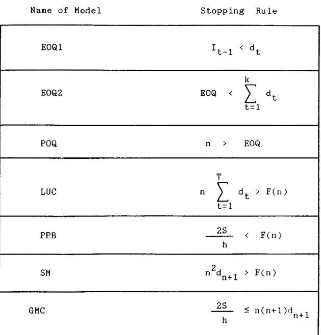
EOQl, E0Q2, POQ, LUC, PPB, SM and GMC heuristic models are

ÖZET

ENVANTER BÜYÜKLÜĞÜ TESBIT PROBLEMLERİNDE KULLANILABİLECEK TEK ÜRÜNLÜ, SINIRSIZ, SEZGİSEL ÇÖZÜM YÖNTEMLERİ

Demet Çapan

İŞ idaresi Yüksek Lisans

Tez Yönetmeni : Yrd. Doç. Dr. Erdal Erel

Ocak 1990, 79 sayfa.

Tek ürünlü, deterministik, periodik inceleme ve sı­

nırsız ürün/envanter modelleri malzeme ihtiyaç planlaması

sistemlerinde yaygın uygulama alanına sahip olmaları açı­

sından, özellikle önemlidirler. Bu tez çalışmasında, konu­

ya ilişkin literatür özetle gözden geçirilmiş, E0Q1, E0Q2,

P0Q, LUC, PPB, SM and GMC isimli sezgisel yöntemlerin

PAGE

ABSTRACT... iv

ÖZET... V LIST OF TABLES... viii

LIST OF FIGURES... ix

CHAPTERS I. 1 .1 . INTRODUCTION... 1

1 .2. CLASSIFICATION OF PRODUCTION/INVENTORY MODELS. . . 1

1.3. MODEL CONSTRUCTION... 2

1.3.1. THE ASSUMPTIONS OF THE MODEL... 3

1.3.2. IMPLICATIONS OF THE ASSUMPTIONS... 5

1.4. PURPOSE OF THE THESIS... 6

1.5. THESIS OUTLINE... 6

II. HEURISTIC SOLUTION MODELS... 7

2.1. ECONOMIC ORDER QUANTITY MODEL... 9

2.1.1. ECONOMIC ORDER QUANTITY 1 MODEL... 11

2.1 .1 .1 . EOQl PROCEDURE... 13

2.1.2. ECONOMIC ORDER QUANTITY 2 MODEL... 14

2.1.2.1. EOQ2 PROCEDURE... 16

2.2. PERIODIC ORDER QUANTITY MODEL... 17

2.2.1. POQ PROCEDURE... 19

2.3. LEAST UNIT COST MODEL... 20

2.3.1. LUC PROCEDURE... 23

2.4. PART PERIOD BALANCING MODEL... 24

2.4.1. PPB PROCEDURE... 28

2.5. SILVER AND MEAL HEURISTIC MODEL... 29

2.6. GROFF MARGINAL COST MODEL... 33

2.6.1. GMC PROCEDURE... 36

III. COMPUTATIONAL DATA SETS FOR COMPARISON OF THE HEURISTIC MODELS... 37

3.1. THE RESULT OF EXPERIMENTATION... 38

3.2. DISCUSSION OF HEURISTIC MODELS WITH RESPECT TO THEIR PROCEDURES... . 3.3. ANALYSIS OF RESULTS... 42

IV. CONCLUSIONS... 45

REFERENCES...48

APPENDIX A. (TABLES)...50

APPENDIX B (LISTING OF THE COMPUTER)... 66

VARIABLES DESCRIPTION ... 67

PROCEDURES DESCRIPTION ... 68

LIST OF TABLES

TABLE NO PAGE NO

2.1 DATA SET FOR THE EXAMPLE... 10

2.2 EOQl EXAMPLE...12

2.3 E0Q2 EXAMPLE...15

2.4 PERIOD ORDER QUANTITY EXAMPLE... 18

2.5 LEAST UNIT COST EXAMPLE... 22

2.6 PART PERIOD BALANCING EXAMPLE... 27

2.7 SILVER AND MEAL EXAMPLE... 31

2 . 8 GROFF MARGINAL COST EXAMPLE... 35

3.1 DEMAND DATA SETS... 51

3.2 COST DATA...52

3.3 SUMMARY OF THE STOPPING RULES OF THE HEURISTICS.... 55

3.4 COST PERFORMANCE OF THE LOT-SIZING MODELS...56

3.5 SUMMARY OF COST PERFORMANCE OF THE LOT-SIZING MODEL.61 3.6 ANOTHER ASPECT OF COST PERFORMANCE OF THE MODELS--- 62

3.7 ANALYSIS OF VARIANCE... 64

3 . 8 THE COMPARISON OF DIFFERENCE BETWEEN ANY TWO GROUP MEANS...65

FIGURE NO PAGE NO

3.1. SCHEMATIC REPRESENTATION OF THE DEMAND PATTERNS....53

CHAPTER I

1 .1 . INTRODUCTION

The production/inventory process can be characterized

by the flow of items into and out of storage points. The

inflow of items is governed by the production or purchase

acquisition, whereas the outflow of items is induced by

demand associated with either customer orders or production

orders. It may be impossible or uneconomical to balance

exactly the inflow with the outflow, and consequently

inventory is created at the storage points.

The production/inventory models which represent this process can be defined in terms of variables and their

interactions. Some of the variables such as demand, cost

and technology are uncontrollable, i.e., they are the

parameters of the model. On the other hand, other variables

such as production and inventory levels are controllable

variables. Interactions can be represented in various forms

such as, inventory balance equations and capacity

constraints.

1.2. CLASSIFICATION OF PRODUCTION/INVENTORY MODELS

The production/inventory models can be classified into

two groups Continuous review refers to the case where

production (or purchase) decisions can be made at any point

in time. In Periodic Review, decisions are made at

If the parameters of the model are known exactly, then the model is said to be a deterministic one, but if the

parameters are random variables with known probability

distributions, then the model is said to be stochastic.

Multi-item models are characterized by the fact that there exist cost, demand and resource interactions among the

items. If there are no such interactions, then it becomes a

single-item model.

If there exists a restriction on resources then the

model is called capacitated, otherwise the model is

considered as uncapacitated.

The models discussed in this study belongs to the

class of single item, deterministic, uncapacitated, periodic

review lot-sizing models. The choice is due to the wide,

spread use of this class of models in MRP setting.

1.3. MODEL CONSTRUCTION

Following are the list of variables used in the

model:

T = Planning horizon.

X^= Production (purchase) quantity at period t, t=l,2,..., T

d^= Demand at period t, t=l, 2, , T

I^= Inventory level at the end of period t, t=l, 2 I = Inventory level at the beginning of the period,

o

The following is the mathematical programming formulation of the model:

Min 2 = ^ [ ( S.y^ + c.X^ ) + h.I^ J

t=l Subject to ^t ^t-1 ^t ■ *^t ^t- « ^t It ^ 0 Xt ^ 0 , y

J ‘

Where M is a large number.

1.2.1. The assumptions of the model:

The model has some important assumptions. These

assumptions simplify the model and allow for mathematical

manipulation and computational feasibility. They are listed

below:

i) Demand is deterministic, i.e., demand quantities are

known for all periods with certainty.

ii) The ordering, unit variable production and unit

inventory carrying costs are deterministic and constant. iii) No shortages are allowed; i.e., for any period, the

iv) Production (or purchase) decisions are made at the beginning of the periods.

v) The unit inventory carrying cost is a linear function

of the inventory level. Also the unit variable production

cost is a linear function of the production level; i.e., any other function is not allowed, because linearity feature of the objective function must be satisfied.

vi) Items are treated as independent items, i.e., there are

no resource, demand or cost interactions among the items.

Solution of the problem above is usually

computationally infeasible for a realistic T, since the

number of constraints and variables are mostly affected by

the size of the problem under consideration. On the other

hand, the problem can be solved with a dynamic programming

approach with much less computational requirements. Such a

formulation was first given by Wagner and Whitin (12).

Although Wagner and Whitin (WW) model gives optimal

solution, it requires relatively high computational effort

in MRP environment; i.e., the WW model searches T(T+l)/2

alternative solution procedures. For that reason, several

lot-sizing heuristic models are proposed in the literature. Their computational requirements are relatively less but

they do not ensure optimality. In this study, it is

examined seven heuristic models and apply them to 35 test data(developed by Kaimann [5]) to find out which of these

1.3.2. IMPLICATIONS OF THE ASSUMPTIONS

The meaning and importance of the assumptions and the implications of relaxing them are briefly discussed below:

(i) If the demands were not deterministic, then it

would necessitate the use of probabilistic distribution

functions for expressing the demand set, in which case a

linear model could not be used, nor could such a model be

deterministic.

(ii) In the heuristic models, variables such as

set-up costs, inventory carrying costs, production costs,

etc. are assumed to be constants. Relaxing this assumption,

would invalidate the use of heuristic models and would

necessitate the use of an optimum finding algorithm such as WW model.

(iii) The assumption of "no shortages" : This

assumption can be relaxed easily, because if it were to be

relaxed then we would have to introduce another cost term

into our objective function and make our evaluations

accordingly, in which case the extra term is the product

of number of shortages and unit shortages cost.

(iv) Production (purchase) decisions are made at the

beginning of the periods. In other words, this is the

"periodic review assumption".

(v) The unit inventory carrying cost is a linear

(vi) The assumption of ” single-item Otherwise,

the problem is multi-item lot-sizing problem. But,

multi-item, uncapacitated problems are also solved for each item by using this model.

1.4. PURPOSE OF THE THESIS

"The single item, deterministic, periodic review and

uncapacitated production/inventory model" is chosen as a

subject for the thesis mainly because of applications in MRP systems, since the production planning environments are generally affected by the decisions to be made on MRP

systems. This thesis is based on comparison of seven

heuristic models to solve lot-sizing problems.

1.5. THESIS OUTLINE

In the introduction chapter, a classification of the

production/inventory models is considered. Chapter I states

variables which are used in the model considered and the mathematical programming formulation of the model is given. The assumptions of the model and their implications are also presented in Chapter I .

The analysis of the available heuristic models with

their assumptions and other structural properties are

presented in Chapter II.

In Chapter III, properties of data sets for

computational comparison of heuristic models are described.

CHAPTER II HEURISTIC MODELS

In the literature, several heuristic models for

determining lot sizes in single item, deterministic and

periodic review models, have been outlined. The optimal

solution to the problem can be obtained by the Wagner and Whitin model(12).

The W/W model is a dynamic programming approach

which uses several theorems to simplify the computations. The algorithm proceeds in a forward direction to determine

the minimum cost policy. Although it finds an optimal

solution, heuristic models are generally used in practice

since computational requirements are quite large. Such

that, the computation time of WW algorithm increases

explonantially relative to heuristic models' computation

times when the size of parameters increases. Thus, various

heuristic models have been developed since 1968. These

heuristic models are computationally more attractive, but

they do not ensure optimality.

The following heuristic models are frequently

referred to in the literature:

1- Economic Order Quantity (EOQ) (1,6,8,9)

2- Period Order Quantity (POQ) (9,10)

3- Least Unit Cost (LUC) (3,8)

4- Part Period Balancing (PPB) (2,7,8,11)

5- Silver and Meal Heuristic (SM) (9,10,11)

The first one is demand-rate oriented and the rest are

discrete lot-sizing procedures. Since the discrete

lot-sizing procedures generate order quantities which equal the sum of demands in an integral number of consecutive

planning periods, they do not create "remnant" stock;

i.e., quantities that would be carried in the inventory

for a length of time without being sufficient to cover

a future period's demands in full.

In some of these models, the order quantity is

fixed while the ordering interval varies; EOQ belongs to

this class. In POQ, on the other hand, the ordering

interval is fixed and the order quantity varies. The

rest, including LUC, PPB, SM and GMC allow both ordering

interval and order quantity to vary. Thus, they have the

capability of coping with the seasonal variability or

lumpiness of the demand. For this reason, the last four

heuristic models are widely used in practice.

In the literature, there are two inventory carrying

cost criteria: " Average inventory carrying cost (AICC)

criterion " and " End of period (EOP) criterion ". The

basic difference between the two criteria can also be

demonstrated in the following manner:

Let H(n) denote the inventory carrying cost for n periods

using the end of period criterion. And let H'(n) denote

the inventory carrying cost for n periods using the average

n H'(n) = h ^ t = l t -n H'(n) = h t=i (t-l) + h n t=i (2. 1) Whereas n H(n) = h ^ (t-l) t=l

As it can be observed, the end of period criterion differs from the average inventory carrying cost criterion

by the second term of E q . (2.1). This term has no effect on

the optimal solution of W/W model since it would

be added identically to all ordering alternatives for

each period. Since optimal solution does not change with

changing the inventory cost criterion, in all heuristic

models end of period criterion is used.

In the rest of this chapter, the basic concepts of

each of the seven heuristic models will be summarized; the

solution procedures will be developed and stated and they

will be applied to a simple set of demand data in lieu of

an example.

2.1. ECONOMIC ORDER QUANTITY MODEL

This model is widely used because of its simplicity.

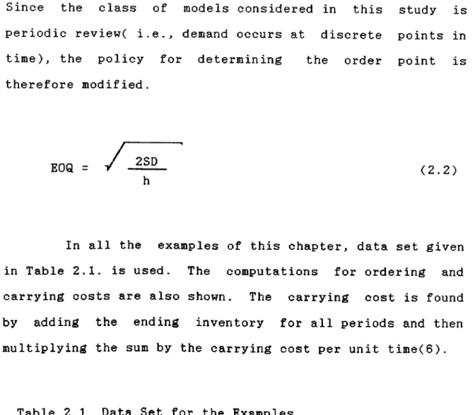
Since the class of models considered in this study is periodic review( i.e., demand occurs at discrete points in

time), the policy for determining the order point is

therefore modified.

EOQ =

/

In all the examples of this chapter, data set given

in Table 2.1. is used. The computations for ordering and

carrying costs are also shown. The carrying cost is found

by adding the ending inventory for all periods and then

multiplying the sum by the carrying cost per unit time(6).

Table 2.1. Data Set for the Examples

period no 1 2 3 4 5 6 7 8 9 10 1 1 1 2

Demand 10 10 15 ₂₀ 70 180 250 270 230 40 0 10

S ::TL 300.

There are two variations of the EOQ heuristic model:E0Q1 and E0Q2.

2.1.1 ECONOMIC ORDER QUANTITY 1 MODEL

This heuristic model places an order whenever the

quantity on hand is less than current demand. A check

is made to see if EOQ equals or exceeds current demand.

If so, the order quantity is the EOQ. If EOQ is less

than the current demand, then the order quantity is

increased to meet the current demand. In brief, production

quantity is set equal to the maximum of EOQ or the

difference between demand at current period and inventory

level at previous period(6).

If

otherwise, = max { ^0« ■ - ^t- 1 }

stopping rule ^

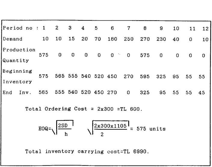
An example illustrating this heuristic model is given Table 2.2. by using EOQl procedure.

Table 2.2 EOQl Example Period no 1 2 3 4 5 6 7 8 9 10 1 1 12 Demand 10 10 15 20 70 180 250 270 230 40 0 10 Production Quantity 575 0 0 0 0 0 ' 0 575 0 0 0 0 Beginn ing Inventory 575 565 555 540 520 450 270 595 325 95 55 55 End Inv. 565 555 540 520 450 270 0 325 95 55 55 45

Total Ordering Cost =: 2x300 =TL 600.

E0Q=> 2SD ' 2x300x1105 L 575 units

h \ ₂

2.1.1.1 EOQl PROCEDURE 1) Initialization, t = 1 , I^= 0, X^= 0, Vt go to 2) X^= max

J

I

/

I

2.1.2 ECONOMIC ORDER QUANTITY 2 MODEL

The EOQ2 model is almost the same as the EOQl. The

only difference is that the E0Q2 is a discrete lot sizing

model. That is, the order quantity is equal to the

cumulative sum of the demand of consecutive periods. But

it is not necessarily equal to the EOQ. In this model,

the ^lot-size is determined by comparing the EOQ with the

cumulative demands at the consecutive periods. The one

which is closer to the EOQ is chosen as the lot size (1). The stopping rule of this heuristic model is as follows:

k EOQ ^ ^ t=l

< I

rule above holds, the order k quantity is taken to be

z

closer to the EOQ.

The following are the definition of symbols used in the E0Q2 procedure :

— p is the current period at which we are making

decision.

— k is the period at which sum of cumulative demand from period p to k just exceeds EOQ.

let,

'pk

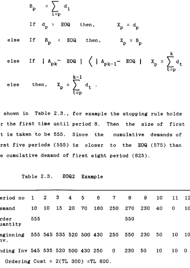
else else else B T = V d. P _{L · 1} If i=p d > EOQ then, X = d P P P If B < EOQ then, X = B P P

If _{1 Ap^- EOQ} 1 ( 1 EOQ

k- 1

then,

t=p

t=p

As shown in Table 2.3., for example the stopping rule holds

for the first time until period 8.Then the size of first

lot is taken to be 555. Since the cumulative demands of

first five periods (555) is closer to the EOQ (575) than the cumulative demand of first eight period (825).

Table 2.3, E0Q2 Example

Period no 1 2 3 4 5 6 7 8 9 10 1 1 1 2 Demand 10 10 15 20 70 180 250 270 230 40 0 10 Order Quantity 555 550 Beginning Inv. 555 545 535 520 500 430 250 550 230 50 10 10 Ending Inv 545 535 520 500 430 250 0 230 50 10 10 0 Ordering Cost = 2(TL 300) =TL 600. Inv. carrying cost =TL 6280

2.1.2.1 E0Q2 PROCEDURE 1) let, p=l, k=l, X =0^ Vt 2) If k ) T then go to else go to 3) If d ) EOQ then, X = d go to P P P else go to 4) Find ^pk’ 5) If / EOQ then, X = B go to P \ P P else go to

6) If I Apj^ - EOQ I ^ I - EOQ | then.

= I

2.2. PERIOD ORDER QUANTITY MODEL

Period order quantity model is based on the

principles of the classic E0Q(9)model. In POQ procedure

the economic ordering interval (EOI) is computed rather

than the economic order quantity. Once the EOI is computed,

the lot-size is taken as the sum of demands during the

economic ordering interval. This heuristic model is

equivalent to the simple rule of ordering *’x months'supply",

but X is computed rather than determined exogenously.

OPH (Orders per horizon) =

EOQ

which is T

^ = I "t

t=i

EOI( economic order interval) =

=min t+EOQ-1, T |· OPH h --i=t If >0) or (d^ =0) Otherwise

I a I = b, b is the largest integer which is greater than

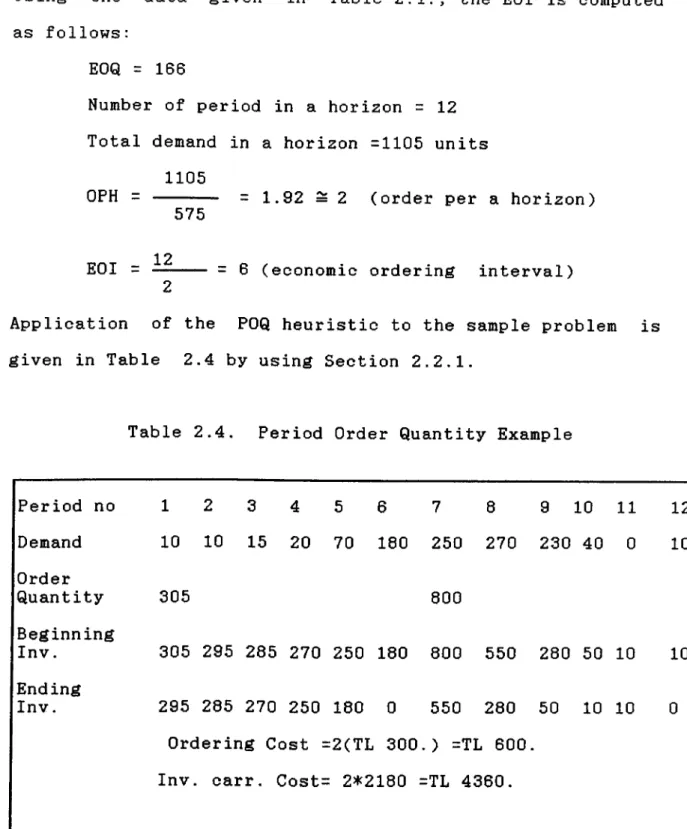
Using the data given in Table 2.1., the EOI is computed as follows:

EOQ = 166

Number of period in a horizon = 12 Total demand in a horizon =1105 units

1105 OPH =

EOI =

575

= 1.92 = 2 (order per a horizon)

12

= 6 (economic ordering interval)

Application of the POQ heuristic to the sample problem is given in Table 2.4 by using Section 2.2.1.

Table 2.4. Period Order Quantity Example

Period no 1 2 3 4 5 6 7 8 9 10 1 1 12 Demand 10 10 15 20 70 180 250 270 230 40 0 10 Order Quantity 305 800 Beginning Inv. 305 295 285 270 250 180 800 550 280 50 10 10 Ending Inv. 295 285 270 250 180 0 550 280 50 10 10 0 Ordering Cost =2(TL 300.) =TL 600, Inv. carr. Cost= 2*2180 =TL 4360.

2 .2 .1 . POQ PROCEDURE

1) Initialization, t=l, X^=0 Vt , Find EOQ, EOI

2) If d^=0 then, t=t+l else compute k^, go to 3) Set ^“^^t 4) Set t=K , t=t+l 5) If t=T go to else go to 6) End

2.3. LEAST UNIT COST MODEL

Least Unit Cost model is based on the minimization

of the "unit cost". In determining the lot-size the LUC

model probes whether the lot-size should be equal to the

first period's demand or whether it should be increased to

cover the demand of the next period and/or the one after

that, etc. The decision is based on the "unit cost" ( i.e.,

set up plus inventory carrying cost per unit) computed

for each of the successive order quantities. The one

with the least unit cost is chosen to be the lot—size.

Derivation of the stopping rule of the LUC heuristic

is as follows (3): UC(n) is defined as the unit cost of

replenishment which covers n period's demand.

UC(n) = n t=i n S + h ^ d^( t-1) t = l (2.3)

The basic idea of the LUC heuristic is to evaluate

Eq.(2.3) for increasing values of n, until the following

condition is satisfied:

UC(n+l) > UC(n) (2.4)

that is, until unit cost starts to increase.

Using Eq.(2.3) and Eq.(2.4), we can obtain

r ^“*"1_{■ ^} 1 _{\ 1} r n n

S + h ) d.( t-1)

)

Last inequality can be expressed as: S n+1 — * Z u t = l

>

I

Z

by defining a counter F(n) as:

F(n) = F(n-l) + (n-l).d^ n= 2,3,...

where

F(l) = and

by substituting F(n) into Eq.(2.5), we can obtain

n+ 1

Z

The equation (2.7) is the stopping rule of the LUC

In summary, the LUC heuristic determines the lot size by evaluating expression Eq.(2.7) for the increasing values of n and adding the future demands to the current lot until

the stopping criterion is satisfied. The same procedure is

repeated for the remaining periods. Application of this

heuristic to the sample problem is given in Table 2.5

by using Section 2.3.1.

Table 2.5. Least Unit Cost Example

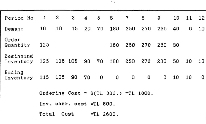
Period No. 1 2 3 4 5 6 7 8 9 10 11 12 Demand 10 10 15 20 70 180 250 270 230 40 0 10 Order Quantity 125 180 250 270 230 50 Beginn ing Inventory 125 115 105 90 70 180 250 270 230 50 10 10 Ending Inventory 115 105 90 70 0 0 0 0 0 10 10 0 Ordering Cost = 6(TL 300. ) =TL 1800.

Inv. carr . cost =TL 800.

2.3.1 LUC PROCEDURE 1) let, p=l, F(0) =0, X^=0 Vt 2) n = l. Since, F(l) =-If p=T then go to else go to 3) If dp < F(l) then, go to else go to 4) Set Xp = dp and p = p+1 go to I 2 5) If p+n-1 = T then, else n=n+l go to X t=P go to P+n-1 6 ) Compute cost = n ^ d^ , F(n) = F(n-l) + (n-l)dp^^ j^ t=p 7) If Cost i F(n) go to else go to p+n-1 8 ) Set, Xp = ^ dt , t=p P = n+1 go to 9) End

2.4. PART PERIOD BALANCING MODEL

PPB heuristic has the objective of minimizing the

sum of set up and inventory carrying cost. It attempts to

reach this objective by trying to equate the total cost

of ordering to the total cost of carrying inventory. This

can be written as follows: n

S ^ h \ ( t~l)

t^i t=i

dividing both sides by h, we obtain

n

t = l ^

(t-1) (2.8)

In the literature(7), S/h is called "The Derived Part Period Value” and some authors call it" The Economic Part

Period (EPP)". It is the inventory quantity which, if

carried in the inventory for one period, would result in

a carrying cost equal to the set up cost. The RHS term,

n

I'

t = l

or as some authors call it, "The Part Period Cost". It is

the number of items held in the inventory for a certain

period of time.

The PPB heuristic selects the order quantity such that The Part Period Cost ( Generated Part Period Value) is

n

< Y . d (t-1)

t = l ^

(2.9)

that is, when the generated part period value is first

greater than derived part period value, new order should

be placed. To determine reorder period and the order

quantity, the generated part period values of the current

and the previous periods are compared with derived part

period value. Reorder period is the successor of the

period at which the derived and the generated part period

values are the closest. Then, the order quantity equals the

cumulative demands up to the preceding period This can be presented as follows:

c When the stopping rule holds ( i.e.,

n h y d,(t-l> -n

1

1

)

then, the first lot—size will be

= n

I

and the reorder period ( or period at which new order is placed) will be :

J

J =

To put the stopping rule in a form which is compatible with that of LUC, the following algebraic manipulation can be made: 2S h n t = l ^ (

2

1 0

and substituting these into Eq.(2.10), we can obtain the stopping rule of PPB heuristic in the following form:

2S

< F(n) (

2

11

Application of the PPB heuristic to the sample problem is illustrated in Table 2.6 by using Section 2.4.1.

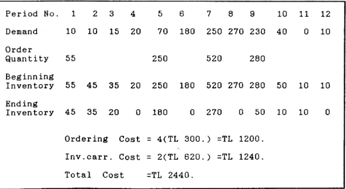
Table 2.6. Part Period Balancing Example Period No. 1 2 3 4 5 6 7 8 9 10 11 12 Demand 10 10 15 20 70 180 250 270 230 40 0 10 Order Quantity 55 250 520 280 Beginning Inventory 55 45 35 20 250 180 520 270 280 50 10 10 Ending Inventory 45 35 20 0 180 0 270 0 50 10 10 0 Ordering Cost = 4(TL 300.) =TL 1200. Inv.carr. Cost = 2(TL 620.) =TL 1240. Total Cost =TL 2440.

2.4.1. PPB PROCEDURE 1) Let, j = l, t = l, X = 0 Vt, F(l) = - ^ , CST = h h 2S 2) If t=T or j=T then, X . = d go to J / . P P=j else t=t+l go to 3) Set k=t-j+l F(k) = F(k-l) + (k-l)d, 4) If F(k) < CST then, go to else go to 5) DIF^ dp (p-j) - F(l) P=J t-1 DIF^_^ = F(l) - ^ dp (p-j) P=j

6 ) If DIF^ < DIF^_j^ then, X. =

t-1 else Xj= ^ dp , j=t P=j go to 7) End

y

2.5. SILVER AND MEAL HEURISTIC MODEL

The basic idea of the heuristic is based on the

minimization of the total cost per unit time. It selects

the order quantity in such a way that the total cost per

unit time is minimized (9). Total cost per unit time can be

expressed as: TCUT(n) ( S + h n 11

I

1

2

1 2

where TCUT(n) is total cost per unit time, n=l,2,3...etc.

is the decision variable duration that replenishment

quantity is to last.

The model of the heuristic evaluates TCUT(n) for

increasing values of n until the following condition is

satisf ied:

TCUT(n+l) > TCUT(n) (2.13)

that is, until total cost per unit time starts to increase.

When this happens, n is selected as the number of periods

that the replenishment will cover. The stopping rule of the

SM heuristic is obtained as follows:

From Eq.(2.12) and Eq.(2.13), we can write

n+1 n

n+1

( S + h (t - D ) > (S + h

t=l n t=i

(t-D)

By dividing both sides of above inequality by h and

I

>

inequality Eq.(2.14) becomes

F(n+1) or F(n) n+1 F(n) + nd n+1 F(n)

>

By rearranging the terms of Eq.(2.15), we can obtain the

stopping rule in the following form (10):

> F<n) (2.16)

The application of this heuristic to the sample problem

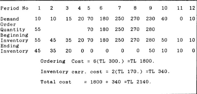
Table 2.7. Silver and Meal Example Period No 1 2 3 4 5 6 7 8 9 10 11 12 Demand 10 10 15 20 70 180 250 270 230 40 0 10 Order Quantity 55 70 180 250 270 280 Beginn ing Inventory 55 45 35 20 70 180 250 270 280 50 10 10 End ing Inventory 45 35 20 0 0 0 0 0 50 10 10 0 Ordering 1Cost = 6(TL 300. ) =TL 1800.

Inventory carr. cost = 2(TL 170. ) =TL 340.

2.5.1. SM PROCEDURE 1) Let, j = l, t = l, X,- = 0 Vt, F(l) = 2) Set k=t-j+l F(k) = F(k-l) + (k-l)d^ go to 3) If t=T then, ^ dp go to P=j else go to 4) If F(k) ^ k d^^j^ then, go to else go to 5) If t=T or j=T then, ^ P=j d go to 8 P __ else t=t+l go to 6 ) Set X.= У d , j=t+l, t=t+l go to J P p=j 7 ) If t=T or j=T then, X.=

V

8 ) End.

2.6. GROFF MARGINAL COST MODEL

This heuristic is based on the marginal costs rather

than the total costs. The traditional EOQ rule is

established by increasing the lot-size as long as the

marginal savings in the ordering cost is greater than the

marginal cost increase in the inventory holding cost. Thus,

the optimal lot-size is reached when the marginal

increase in ordering cost equals to the marginal increase

in inventory holding cost. By using the same analogy,

this heuristic adds the future demands to the lot-size as

long as the marginal increase in inventory holding cost

for the period is less than the marginal decrease in

ordering cost (11).

The marginal cost decrease for adding n+lst. period's

demand to the lot is the decrease in ordering cost per

period, or

n n+1 n(n+l)

(2.17)

Groff's model approximates the discrete inventory depletion

to the uniform inventory depletion. Inventory holding

cost for a horizon of n periods and n+1 periods can be determined as follows:

H(

n n

" ' 7 ' h.n h

and n+1 H(n+1)= — ( — (n+1) n+1 2 • ' I ''t t=i n+1 t=i

then, the marginal cost increase from adding n+lst. period's demand to the lot is

n+1 n

H(n+1) - H(n) = — h ( ^ d^ - ^ d^) = ~

2 t^l t^l ^

h (2.18)

Therefore, the stopping rule of Groff's model will be

(n+l)n

h d

n+1 (2.19)

i.e., the marginal decrease in ordering cost is less than or equal to the marginal increase in inventory holding cost(4). The inequality (2.19) can be simplified and presented in the following form:

2S

i n(n+l)d

n+1 ( 2 . 2 0 )

Application of the heuristic to the example problem is given in Table 2.8 by using GMC procedure.

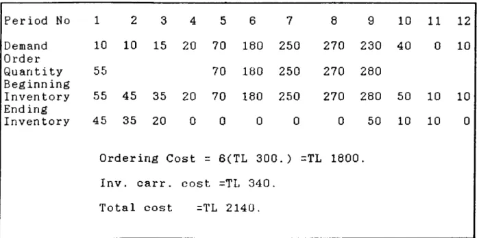
Table 2.8. Groff Marginal Cost Model Example Period No 1 2 3 4 5 6 7 8 9 10 11 12 Demand Order 10 10 15 20 70 180 250 270 230 40 0 10 Quantity Beginning 55 70 180 250 270 280 Inventory End ing 55 45 35 20 70 180 250 270 280 50 10 10 Inventory 45 35 20 0 0 0 0 0 50 10 10 0 Ordering Cost = 6(TL 300.) =TL 1800. Inv. carr. cost =TL 340.

2.6.1. GMC PROCEDURE 1) Let, j=l , t=l , T 2) If t=T then, =

Σ

1

CHAPTER III

3.1. COMPUTATIONAL DATA SETS FOR COMPARISON OF THE HEURISTIC MODELS

In general, there are two criteria to compare these

heuristic models:(1) total cost of set-up and carrying

inventory. (2) Computation time of heuristic model

procedure. The second measure is a measure of the effort to

find solutions. For the first criterion, the comparison

is made in order to find the deviation of their total costs

from the optimal solution. In other words, W/W model is

used as a benchmark to measure the cost performance of the

heuristic models. As the performances of the heuristic

models are different under different data sets, it is

hard to measure their performances exactly. The difficulty

lies in the fact that the performances of the heuristic

models vary, depending upon the variability of demand.

However, Kaimann (5) has prepared data sets which

reduce this difficulty. These data sets which are given in

Table 3.1 and 3.2 (in the Appendix A) have been prepared by

using five different sets of cost data and seven different

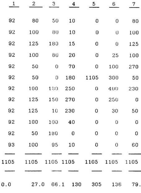
sets of demand data. As it can be seen from Figure

3 .1., the demand data represents a variety of possible demand patterns that will encompass a wide range of the

possible demand situations. Each of these demand patterns

have the same total demand for the year, namely 1105 units.

There are 35 examples, all derived from the seven

demand patterns and the five ordering costs. Totally 35

test problems are solved for each heuristic model.

The performances of all the heuristics are measured by using these data sets, and by comparing their results with those yielded by W W .

3.2. THE RESULT OF EXPERIMENTATION

Several heuristic models for determining the lot-size in single— item, deterministic and periodic review models

have been outlined. These find extensive use in Material

Requirements Planning systems.

Each of them starts with the current period and

scans successive periods until the stopping rule is

satisfied. Then an order is placed to satisfy the total

requirements up to the stopping period, except for EOQl in

which the order quantity is equal to EOQ. Then the same

procedure is repeated for the remaining periods. Although

the basic idea is the same, the stopping rules which

characterize the heuristics are different. In this study,

Almost all of the lot-sizing heuristics are based on

the rationale underlying the EOQ, that is, they are

developed by using one of the properties of the optimal

solution of the EOQ. These properties may be summarized as

follows:

- minimization of total costs per unit which is the objective of the LUC heuristic.

- minimization of total costs per unit time which is the objective of the SM heuristic.

- adding to inventory lot until the marginal

increase in inventory holding costs is equated to the

marginal decrease in ordering costs, which is the basic

idea of GMC model.

- equating the total cost of ordering and the total

inventory carrying cost which is the basic idea of PPB

heuristic.

It is possible to conclude that all heuristics are developed based on the EOQ, each of them is approximated different approach to problems of cost minimization.

In this study, heuristic models for the single item, periodic review and deterministic model are compared and solutions are obtained in each case using the standard data

sets available in the literature. In addition, all the

heuristic models are analyzed with respect to structural

Moreover, an interactive package program which

contains all the lot-sizing models are prepared. If the

problem is solved by using computer, the user can use the interactive package program which is written in TURBO PASCAL

language. The test problems are solved on a CORONA

PC / XT-40 personal computer (in the Appendix B).

The results of 35 examples are given in Table 3.4.and

Table 3.5.(Appendix A): The former exhibits the cost

performance of the lot-sizing models, and the latter Table

summarizes cost performance for each heuristic models.

As the Tables clearly indicate, since the WW model provides optimal results, it can be used as a yardstick to measure the comparative cost performance of the other lot sizing models.

The results indicate that the solution yielded by WW is best approximated by the by SM and by the GMC models.

By using these heuristics, processing time can be

decreased approximately twice. While the average percentage

deviation of the results of SMH and GMC from the optimal solution is about .028%, the average of the said deviation

for the other five heuristics are 1.523% .

3.2. DISCUSSION OF HEURISTIC MODELS WITH RESPECT TO

THEIR PROCEDURE

According to the result of 35 test problems,

V It- 1 = 0

It is known that for these type of problems, WW

model gives the optimal solution, the most important result

of which can be expressed as below:

(3.1) The expression (3.1) is stated that if the quantity of inventory carried to the next period is positive then the

production at that period must be zero. Or, if the

production quantity is greater than zero at any period then

the carried inventory to this period must be zero. This is

not the case in other discrete heuristic models. The SM

heuristic is discrete lot-sizing model. For that reason,

SM heuristic does not create remnant stock.

One of the features of EOQl and E0Q2 models is

its consideration of total demand, which can be considered

a weakness, because in lot-size determination problems the

crucial variable is not total demand, but rather demand variation over the periods.

POQ has the similar property and weakness of

considering total demand rather than demand variation over

periods, but it determines an ordering interval.

However, it makes a simple division without taking into

consideration demand variation period by period as is the case in SM and GMC models, and therefore the former yields

higher cost results as compared to the latter. And its

ordering interval can cause the increase in total cost by

LUC, PPB, GMC and SM heuristics allow both ordering

interval and order quantity to vary. Thus they have the

capability of coping with the seasonal variability

or lumpiness of the demand. Although the basic approach of

them is same, SM heuristic has a better stopping rule:

It considers the minimization of total costper unit time.

3.3. ANALYSIS OF RESULTS

The seven heuristics (i.e., EOQl, E0Q2, POQ, LUC,

PPB, SM and GMC) are tested by solving 35 test problems for

each. As a result, totally 245 problems are solved by

using an interactive package program which is written in

Turbo Pascal Language and the results are depicted in Table

3.4. To facilitate a nalysis of these results. Table 3.6 is

constructed. This Table presents the ratio of the total

costs of set-up and inventory carrying found for each

heuristic model for test problems when compared with WW algorithm.

These results are statistically analyzed via the

one-way analysis of variance(ANOVA) technique. ANOVA method

is used to examine if there are any significant differences

between these heuristic models. Thus, the equivalence of

the seven heuristics' total costs of set-up and inventory

^2 ^ 3" ^ 4" ^ 5“ ^ 6“ ^7

: At least one of the heuristics' total costs set-up

and inventory carrying means differs from the rest.

The result of ANOVA output can be seen Table 3.7 in

Appendix. As it can be observed from Table 3.7 the

p-value^ for corresponding to F-ratio = 36.282 and is

approximately equal to zero. From the Table, we can reject or accept the null hypothesis either by looking at the F

statistic or by looking at p-value. The observed F-test

ratio is so big and p-value is so small that we can

conclude that there is sufficient evidence to reject the

null hypothesis. Thus, it can be concluded that means of

the heuristics' total costs of set-up and inventory carrying significantly differ from each other.

It should also be concluded which heuristic models

have shown better performances than the others. Then,

the equivalence of the any two pair heuristics' total costs

of set-up and inventory carrying them is set as an

alternative hypothesis. That is.

H : iJ,=

0 1 J

«A ^ ''j

The results of t-test computations for any two

heuristic-model pairs are given on Table 3.8 , results

^The p-value for a test of hypothesis is the probability

indicate that there are statistically significant differences between SM, GMC on one hand,and the other five

2

heuristic on the other . It can be concluded that the

performances of SM and GMC are better than other heuristics and a similar conclusion is indicated by confidence interval figures which are closer to l(on Table 3.6.) for SM and GMC.

CHAPTER IV.

CONCLUSIONS

In this thesis, performances of heuristic models for

single-item, deterministic, periodic-review lot-sizing

problems are compared with the application to the Material

Requirement Systems, since the production planning

environments are generally affected by the decision to be made on MRP systems.

The mathematical programming formulation of

lot-sizing problems are indicated and their assumptions

are shown. Then the nature, meaning and importance of these

assumptions and the implications of them are briefly

d iscussed.

The method which yields an optimal solution for

single-item, deterministic, periodic review and

uncapacitated lot-sizing problems was developed by Wagner

and Whitin in 1958, who developed a procedure that

guarantees an optimal solution in terms of minimizing the

total cost of replenishment and carrying inventory. However

the procedure are received exteremely limited acceptance in

practice, because of the relatively complex nature of its

algorithm, the considerable computational effort required

for its use and the possible need for a well-defined ending point for the demand pattern.

Instead, simpler heuristic models are resorted which result in reduced control costs that more than offset

any extra replenishment or carrying costs that their use

may incur. A scan is made of the relevant literature

and seven of the heuristic models which yield best

results are selected for a test of their performance:

These are EOQl, E0Q2, POQ, LUC, PPB, SM and G MC.

The basic concepts of each of these heuristic models are briefly summarized and a sample problem is solved for each.

Since the performances of heuristic models are

different under different data sets, it is difficult to

measure their performance exactly, because of the fact that

the performances of the heuristic models vary depending

upon the variability of demand. However, Kaimann (5) had

prepared data sets( Table 3.1 and 3.2 ) which reduced

this difficulty; and these data sets are used in our study

for evaluating and comparing the performance of the

heuristics selected.

A total of 35 test problems are made for each

heuristic model, they are compared by using the standard

Kaimann data sets. An interactive package programme

written in TURBO PASCAL language which contains all the

lot-sizing procedures are prepared. The results of the 35

examples (tests) are given in Table 3.4 and Table 3.5,

According to the Table 3.7., for F-ratio=36.282 and

p-value is approximately equal to zero. Thus, the observed

F-test ratio is so big and p-value is so small. Thus, we

can conclude that there is sufficient evidence to reject the

null hypothesis. It can be concluded that the performance

of the each heuristic differs from each other.

Having shown that the mean of the results obtained

from 35 test cases are differed for each heuristic,

t-tests are made for each pair of the seven heuristic

models examined.

The results of t-tests for any two heuristic-model

pairs ( Table 3.8) indicate that there are significant

differences between SM and GMC on the one hand, and the other five heuristics on the other.

When the mean of the results obtained from the

former four heuristics and EOQl ( expressed in terms of

their ratio to the results obtained from WW algorithm ) are compared to the analogue figures yielded by SM and GMC,

extremely small p-values were obtained, the largest being

about 0.00015.

Thus this study reconfirms that the performances of

SM and GMC are better than those the other heuristics

tested

Finally, for further research, a better solution

model can be found by applying a more realistic stopping

rule to the SM and GMC models, which have approximated the

REFERENCES

1) Berry, W.L. "Lot Sizing Model for Requirement Planning

Systems : Framework for Analysic " Production and Inventory

Management, 2nd Qtr, p p . 19-34, 1972.

2) Dematteis, J.J., " An Economical Lot Sizing Tecnique:Part

Period Algorithm " IBM System Journal, Vol.7, p p . 30-38,

1968

3) Gorhom,J., " Dynamic Order Quantities ", Production and

Invetory Management, Vol.9, p p . 75-59,1981.

4) Groff, G.K., "A lot sizing Rule for Time-Phosed Component

Demand ", Production and Inventory Management, Vol.20, p p .

47-53,1976.

5) Kaimann, R.A, " EOQ vs Dynamic Programming which one to

use for Inventory Ordering ". Production and Inventory

Management, 4th Qtr., 1969.

6 ) Mitra, A, Cox, J.F. Blackstone, J-H., and Jesse, R.R., "A Reexamination of Lot sizing Procedures for Requirement

Planning Systems: Some Modified Rules ", Int.J.Prod. Res.

1983, Vol. 21, No:4, P P . 471-478.

7) More, S-M, " MRP and Least total Cost Method of Lot

sizing ", Production and Inventory Management, Vol. 15,

pp. 57-71, 1974.