A re-examination of the effectiveness of priority rules in a dynamic job shop environment

(1)

к Ш '- І І і М І Щ Щ і i f - Î İ I Ш ' : r i Â i î î ^ Ш Ш - 1 i:' S ü t ; : В ІѴ ІІѲ ІЙ Ш Т 41% . , ·4 . - j iw . w ’ i ' ^ Ж Ш ЕЕШ Ш ■ : . : ^•·· ; wfiiJi W ···

/ 5 ? -J*

(2)

A RE-EXAMINATION OI< THE EIPECTIVENESS OF

PRIORITY RULES IN A DYNAMIC JOB SHOP

ENVIRONMENT

A I I I BS IS

SUBMITTED TO THi;<: d e p a r t m e n t o f i n d u s ir i a l

ENGINEERING

AND THE INSTHTHE OF ENGINEERING AND SCIENCE OF BILKEN r UNIVERSITY

IN PARTIAL FULFILI.MENT OF THE REQUIREMENTS FOR n IE DEGREE OF

MAS I'liR OF SCIENCE

'I'ahar lxjini ,,, , ,

>"':)iiiy,n9'97

(3)

T S

í::

• Lii5

^ Q (Ti, ÍJ

(4)

I certif}' that I have read this thesis and that in iny opinion it is fully adequate, in scope and in quality, as a thesis for the degree of Master of Science.

Assoc. Prof. İhsan Sabuncuoğlu (Advisor)

I certify that I have read this thesis and that in my opinion it is fully adequate, in scope and in quality, as a thesis for the degree of Master of Science.

z i M .

Assoc. Prof. Erdal Erel

1 certify t!:at I have read this thesis and that in my opinion it is fully adequate, in scope a;·.:' in quaiity, as a thesis for the degree of Master of Science.

Asst. Prof. Selim Aktiirk

Approved by the Institute of Engineering and Sciences:

Prof. Mehmet Bai%vy

(5)

ABSTRACT

A RE-EXAMINATION OF 'H IE EFFECTIVENESS OF PRIORITY RULES IN A DYNAMIC JOB SHOP ENVIRONMENT

lahar Lejmi

M.S. in Industrial Engineering

Supervisor; Assoc. Prof. İhsan Sabuncuoğlu July, 1997

III dyiiaiuic job .shop .sdiccliiliiig li(cra(urc, an cxicnsivc research clioil lias been spent to study the performance of priority rules, wliich play an important role to manage scheduling tasks in real life manufacturing systems. This study extends the previous research on priority rules by investigating the effect of due date, processing time, and load variation on the pei (drmance of some well used priority rules in a Job shop environment. Furthermore, tliis study will analyze the performance of the rules under the due window approach. The performance of the rules will be measured in terms of two regular criteria: mean flow time and mean tardiness. In addition, with the incieasing emphasis on using non regular measures, we further study the performance of the rules with respect to the mean absolute deviation (MAD) criterion. Finally, we propose two new rules that perform quiet effectively for the MAD criterion.

Keywords; Job Shop Scheduling, Priority rules. Due Window, MAD.

(6)

ÖZET

DİNAMİK ATELYE T l V İ ÜRETİM ORTAMINDA ÖNCELİK KURALLARININ ETKİNLİĞİNİN TEKRAR İNCELENMESİ

Fallar lejmi

Endüstri Mühendisliği Bölümü Yüksek Lisans Tez Yöneticisi: Doç. Dr. İhsan Sabııncııoğlıı

'Feınmuz, 1997

Dinamik atelye tipi üretim sistemleri çizelgeleme literatüründe, üretim sistemlerinin çizelgelenmesinde önemli bir rol oynayan öncelik kurallarının performansı üzerine yoğun araştırmalar yapılmıştır. Bu çalışma teslim tarihi, işleme süresi ve yük çeşitliliğinin atelye tipi üretim ortamında çok kullanılan bazı öncelik kurallarının performansına etkisini araştırarak bu konudaki çalışmaları genişletmiştir. Ayrıca bu çalışmada öncelik kurallarının performansı "ürün teslim zaman aralığı" yaklaşımı kullanılarak analiz edilmiştir. Bu kurallarının performansı ortalama akış süresi ve ortalama gecikme "düzenli" kriterleri kullanılarak ölçülmüştür. Buna ek olarak "düzenli olmayan" ölçümlere önemin artması göz önüne alınarak, öncelik kurallarının performansı ortalama mutlak sapma kriterine göre de araştırılmıştır. Son olarak, ortalama mutlak sapma kriteri için iyi performansı gösteren iki öncelik kuralı geliştirilmiştir.

A nahtar Sözcükler; Atelye Tipi Üretim Sistemi, Çizelgeleme Öncelik Kuralı, Ürün Teslim Zaman Aralığı, Ortalama Mutlak Sapma.

(7)

(8)

ACKNOWLEDGMENT

T would like to express my gratitude to Assoc. Prof. İhsan Sabuncuoğlu due to his supervision, assistance and understanding throughout tlie development of this thesis.

1 would like also to expiess my thanks to Assist. Prof. Selim Aktiirk and Assoc. Prof. Erdal Erel for their keen interest to the subject matter and accepting to read and review this thesis.

My special thanks to all my friends and specially to Didem Kuşaksızoğlu for their morale support and encouragement.

Finally, I would like to express my endless love to my family and specially to my mother, who came to attend the presentation of this thesis.

(9)

List of Figures

FIGURE 4-1: ILLUSTRATION OF TYPH-I, TYPE-II AND OVERALL DV EFFECTS... 25

FIGURE 4-2: MF VERSUS DUE DATE VARIATION/ EXP. COND. 1... 28

FIGURE 4-3: MF VERSUS DUE DATE VARIATION/EXP. COND. 2 ...28

FIGURE 4-4: MF VERSUS DUE DATE VARIATION/ EXP. COND. 3 ...29

FIGURE 4-5: MF VERSUS DUE DATE VARIATION/ EXP. COND. 4 ...29

FIGURE 4-6: MT VERSUS DDV TYPE I EFFECT/ EXP. COND. 1... 31

FIGURE 4-7: MT VERSUS DDV TYPE-l EFFECT/ EXP. COND. 2... 31

FIGURE 4-8: MT VERSUS DDV TYPE-I EFFECT/ EXP. COND. 3...32

FIGURE 4-9: MT VERSUS DDV TYPE-I EFFECT/ EXP. COND. 4 ...32

FIGURE 4-10: MT VERSUS DDV TYPE-I EFFECT/ EXP. COND. 5 ... 33

FIGURE 4-11: MT VERSUS DDV TYPE-1 EFFECT/ EXP. COND. 6... 33

FIGURE 4-12: MT VERSUS DDV TYPE-I EFFECT/ EXP. COND. 7 ... 34

FIGURE 4-13: MT VERSUS DDV TYPli-I EFFECT/ EXP. COND. 8...34

FIGURE 4-14: MT VERSUS DDV OVERALL EFFECT/ EXP. COND. 1 ... 38

FIGURE 4-17: MT VERSUS DDV OVERALL EFFECT/ EXP. COND. 4 ... .39

FIGURE 4-20: MT VERSUS DDV OVERALL EFFECT/ EXP. COND. 7 ...41

FIGURE 4-21: MT VERSUS DDV OVERALL EFFECT/ EXP. COND. 8 ...41

(15)

LIST OF FIGURES xm

FIGURE 5-1: MF VERSUS PROCESSING TIME VARIATION/ EXP. CONU. I ...52

FIGURE 5-2: MF VERSUS PROCESSING TIME VARIATION/ EXP. COND. 2 ...52

FIGURE 5-3: MF VERSUS PROCESSING TIME VARIATION/ EXP. COND. 3 ...53

FIGURE 5-4: MF VERSUS PROCESSING TIME VARIATION/ EXP. COND, 4 ...53

FIGURE 5-5: MT VERSUS PROCESSING TIME VARIATION/ EXP. COND. I ...54

FIGURE 5-6: MT VERSUS PROCESSING I'lME VARIATION/ EXP. COND. 2 ...54

FIGURE 5-7: MT VERSUS PROCESSING TIME VARIATION/ EXP. COND. 3 ...55

FIGURE 5-8: MT VERSUS PROCESSING TIME VARIATION/ EXP. COND. 4 ...55

FIGURE 6-1: ILLUSTRATION OF RANDOM ARRIVAL RATE... 60

FIGURE 6-2: ILLUSTRATION OF SEASONAL ARRIVAL RATE...60

FIGURE 6-3: ILLUSTRATION OF INCREASING ARRIVAL RATE...62

FIGURE 6-4: ILLUSTRATION OF DECREASING ARRIVAL R A 7E ...62

FIGURE 6-5: MF VERSUS LV/ APPROACH I / TIGHT DUE DATES (K =2.6)... 72

FIGURE 6-6: MF VERSUS LV / APPROACH I / LOOSE DUE DATES (K =4.5)...72

FIGURE 6-7: MF VERSUS LV / APPROACH 2 / TIGHT DUE DATES (K =2.6)...73

FIGURE 6-8: MF VERSUS LV / APPROACH 2 / LOOSE DUE DATES (K =4.5)...73

FIGURE 6-9: MT VERSUS LV / APPROACH 1 / TIGHT DUE DATES (K=2.6)...74

FIGURE 6-10: MT VERSUS LV / APPROACH I / LOOSE DUE DATES (K =4.5)...74

FIGURE 6 -1 1: MT VERSUS LV / APPROACH 2 / TIGHT DUE DATES (K=2.6)...75

FIGURE 6-12: MT VERSUS LV / APPROACH 2 / LOOSE DUE DATES (K =4.5)... 75

FIGURE 7-1: MT VERSUS DUE DATE INFORMATION CATEGORIES/ EXP. COND 1...80

FIGURE 7-2: MT VERSUS DUE DATE INFORMAllONS CATEGORIES/ EXP. COND. 2... 80

FIGURE 7-3: MT VERSUS DUE DATE INFORMATION CATEGORIES/ EXIF COND. 3...81

FIGURE7-4: MT VERSUS DUE DATE INFORMATION CATEGORIES/ EXP. COND. 4 ...81 FIGURE 8-1: ILLUSTRATION OF EARUNESS AND TARDINESS UNDER THE DUE

(16)

LIST OF FIGURES XIV

WINDOW APPROACH...85

FIGURE 8-2: MAD VERSUS DUE DA'l E INFORMATION/ EXP. COND. 1 ... 94

FIGURE 8-3: MAD VERSUS DUE DAH· INFORMATION/ EXP. COND. 2 ...94

FIGURE 8-4: MAD VERSUS DUE DA1 li INFORMATION/ EXP. COND. 3 ...95

(17)

List of Tables

TABLE 2-1: MATHEMATICAL DESCRIPTION OF PRIORITY RULES USED IN THE

STUDY... 13

TABLE 3-1: DUE DATE TIGHTNE-SS PARAME'IER K VALUES...19

TABLE 4-1: CORRESPONDING T, EQUATIONS TO DUE DATE VARIATION EFFECT TYPES... 25

TABLE 4-2: TYPE-I EFFECT / SUMMARY OF RLtSULTS... . 36

TABLE 5-1; PROCESSING TIME VARIATION SIMULATION RESULTS FOR M F...48

TABLE 5-2: PROCESSING TIME VARIATION SIMULATION RESULTS FOR MT...49

TABLE 6-1: MF SIMULATION RESULTS FOR APPROACH 1...65

TABLE 6-2: MF SIMULATION RESULTS FOR APPROACH 2...66

TABLE 6-3: MF SIMUt-ATION RESUI . PS FOR APPROACHES 3 AND 4 ... 67

TABLE 6-4: MT SIMULATION RESULfS FOR APPROACH 1 ... 68

TABLE 6-5: MT SIMULATION RESUL'l’S FOR APPROACH 2 ... 69

TABLE 6-6: MT SIMULATION RESULTS FOR APPROACHES 3 AND 4 ... 70

TABLE 8-1: ME, MT AND MAD SIMULATION RESULTS UNDER DUE WINDOW APPROACH... 88

TABLE 8-2 : STANDARD DEVIATION OF EARLINESS (SE), TARDINESS(ST) AND ABSOLUTE DEVIATION (SAD) SIMULATION RESULTS... 90

TABLE A -I: MF SUMMARY OF RESULTS... 116

TABLE A-2: MF SUMMARY OF RESULTS (CONTINUED)...117

TABLE A-3: MF SUMMARY OF RESULTS (CONTINUED)... 118

(18)

LIST OF TABLES XVI

TABLE A-4; MF SUMMARY OF RESULTS (CONTINUED)... 119

TABLE A-5: TYPE I EFFECT / MT SUMMARY OF RESULTS... 120

TABLE A-6: TYPE I EFFECT / MT SUMMARY OF RESULTS (CONTINUED)... 121

TABLE A-7: TYPE I EFFECT/ MT SUMMARY OF RESULTS (CONTINUED)... 122

TABLE A-8: TYPE I EFFECT/ MT SUMMARY OF RESULTS (CONTINUED)... 123

TABLE A-9: DV OVERALL EFFECT / MT SUMMARY OF RESULTS... 124

TABLE A-10; DV OVERALL EFFEC IV MT SUMMARY OF RESULTS (CONTINUED)... 125

TABLE A -11: DV OVERALL EFFECT / MT SUMMARY OF RESULTS (CONTINUED)... 126

TABLE A-! 2: DV OVERALL EFFECl' / MT SUMMARY OF RESULTS (CONTINUED)... 127

TABLE A -13: THE DUE WINDOW APPROACH / MT SUMMARY OF RESULTS... 128

(19)

Chapter 1 Introduction

The job shop scheduling problem may be characterized as one in which a number of jobs, each comprising one or moie operations to be performed in a specific sequence on specified machines and requiring certain amounts of time, are to be processed. The objective usually is to find a processing older or a scheduling rule on each machine for which a chosen measure of performance is optimal. In the common industrial setting, the scheduling problem is a dynamic one in that jobs arrive at random over time. Analytical solutions to this pioblem have been concerned with the derivation of the steady state joint probability distributions of the job queue sizes at the various machines in the shop, and the determination of the impact of different .scheduling rules on the behavior of the job shop viewed as a network of queues. The analytical approach has proved to be extremely difficult, even with several limiting assumptions, in the face of the difficulties associated with analytic techniques, researchers in this area have relied on computer simulation of real or repre.sentative job shops to study the dynamic .scheduling problem.

(20)

Research on the dynamic job sclieduling problems have been intensive during the last three decades. Due to the difficulty encountered in solving such problems, researchers and practitioners have used priority rules, which are essentially suboptimal, though nevertheless effective and simple in their application. Consequently, priority rules have been a source of interest to many researchers in this area. One of the questions that researchers try to find an answer to, is when and how priority rules are most effective? In order to find an answer, priority rules have been studied within a large variety of job shop environments. Due to the complexity of real job shops structures, researchers have resorted to simplify their job shop models by ignoring the variations that some job shop factors can undergo in i eal life situations. Since, such assumptions may not fit to all real situations, practitioners have been always suspicious to the claiiried best performing rules in those studies.

In this thesis, we relax some of these assumptions by considering the variation in some job shop factors. We focus on three factors: job due dates, processing times, and system work load. We expect that variation in these factors can liave considerable negative impact on the priority rules. Hence, we investigate the effect of the.se variations on the effectiveness ol some well known priority rules in terms of two common regular measures. Mean Flow time (MF) and Mean Tardiness (MT). The aim is to set higher confidence in the use of priority rules by practitioners, and open new directions of research in the study of priority rules.

CHAPTER 1. INTRODUCTION 2

In manufacturing industries, a due date is often considered as an interval in time rather than a point in time. Namely, for each job to be processed on the machine, there is an earliest due date and a latest due date. Any job finished after its latest due date is considered tardy, and any job finished before its earliest due date is considered early. The time between its earliest and latest due date is the due window. The use of due windows in practice seems more attiactive than using single point due date

(21)

estimates. Then, one questions whether priority rules would also be better performing under the due window approach. In this thesis we test some well known due date based rules using the due window approach. We aim to find out if there is some advantage of the due window over the single point due date from a priority rule perspective.

For many years, scheduling research focused on single pciibrmance measures, that are referred to as regular measures, that are nondecreasing in job completion times. Most of the literature deals with such measures as MF, M l’, mean lateness and proportion of tardy jobs, etc. However, the emphasis has changed with the current interest in Just-In-Time (JIT) pioduction, where an ideal schedule is one in which all jobs Finish exactly on their due dates. That is, both earliness and tardiness should be penalized. This can be translated in a non regular measure, such as the absolute deviation of job completion times, MAD. In this thesis, we further extend the work done under the due window approach by testing the rules with respect to MAD. Our objective is to investigate their performances in terms of a non regular measure. In addition, we develop two new rules and test for MAD.

CHAPTER]. INTRODUCTION 3

The rest of this thesis is oiganized as follows. In chaptei· 2, we present the relevant literature. In chapter 3, we introduce our model and the experimental conditions under which experiments are conducted. In Chapter 4, we present the results of our simulation experiments on the effect of due date variation on the effectiveness of priority rules. In chapters 5 and 6, we present the studies on the effect of processing time variation and load variation on the effectiveness of the rules. In chapter 7, we test the rules under the due window approach. In chapter 8, we analyze the due window approach for the non regular measure MAD. In addition, we introduce two new rules and show their supeiiority to other rules with respect to MAD. Finally, the concluding remarks and further research directions are outlined in the conclusion section.

(22)

Chapter 2

Literature Review

This chapter focuses primarily on the modeling and experimental considerations through previous dynamic job sliop scheduling studies. Initially, we state the basic assumptions that are followed by most of the researchers in the area. Then we give the relevant studies on some job shop factors. Finally, we present a brief survey of some well known rules considered in the dynamic job shop environments.

2.1 Assumptions

The following assumptions (R. Ramasesh (1990)) are generally made in most studies: 1. No rework of jobs on any machine.

2. Each job visits a machine only once.

3. No alternative routing of jobs, i.e. each job Vv'ill follow a unique but randomly chosen, machine visitation sequence.

(23)

5. Sequence independent setup limes. 6. Zero transit between niaclnnes. 7. No assembly operations. 8. Deterministic job due dates

9. Deterministic processing times, usually derived from a distribution function. 10. Uniform work load level ovei lime.

2.2 Arrival Process

Most of the studies assume that I he arrival of the jobs to the shop follow a Poisson process. There is some theoretical evidence to support this assumption besides its widespread use in queuing theory. Eissentially, Poisson distribution has been shown to be a good approximation to the ai l ival process if the different sources generating job arrivals to shop are statistically independent (Albin (1982)). Several other distributions such as Erlang (Will)iecht and Presscott (1969)), uniform, geometric, binomial (Elvers (1974)), and empirical (Rowe (I960)), have also been used. Elvers (1974) studied the sensitivity of Ihe relative effectiveness of the job shop scheduling rules with respect to 16 different ai rival disti ibutions and reported that the arrival rate distribution does not affect the relative performance of scheduling rules in the job shop.

2.3 Operation Times

CHAPTER 2. LITERA TV RE RE VIEW 5

Operation times, i.e. the times of sctiq) and for processing are set when the jobs arrive at the job shop. Most studies use an exponential distribution for the set up and processing times. Set up times aic usually assumed to be sequence independent and

(24)

thus combined with the processing times. Some studies have usctl other distributions such as the normal (Eilon and Cotteril (1968)), Poisson ( Conway, Johnson and Maxwell (I960)) and Erlang (Wilbrecht and Presscott (1969)). Jones (1973) (bund out that the performance of the ciilferent scheduling rules with res|)ccl to the idle time percentage measure would be cliiicrcnt if normal disti ibution was used instead of the exponential. Shannon’s (1979) expeiirnents with three different processing time distributions; exponential. Erlang and uniform, showed that the nature of processing time distribution significantly affect the performance of the scheduling rules. An interesting observation from both these studies is that the use of the exponential distribution tends to favor the SPT (Shortest Processing time) rule. This could be attributed to the fact that SPT rule avoids tying up the machines with one of the very long operations which is possible when draws are taken from an exponential distribution.

CHAPTER 2. LITERATURE REVIEW 6

2.4 Number of Machines Visited and Routing

In most simulation models of the hypothetical job shops, the number of machines visited by any job is small ranging from 4 to 9; although a study by Baker and Dzielinsky (1960) investigated shops with 9-30 machines. Simulation of the real world job shops typically have comprised a much larger number of machines, for example Rowe’s study (1960) included 85 machines. The central concern in the simulation research using simulation research using models of hypothetical job shops is whether the number of machines is adequate to capture the complexity associated with a multi machine job shop. Baker and Dzielinsky (1960) and Nanot (1963) investigated job shops with different number of machines and concluded that the size of the job shop did not significantly affect the relative performance of the scheduling

(25)

rules. Wilbrecht and Prescott (1969) demonstrated that 6 machines were adequate to represent the complex structure of a job shop.

2.5 Due date Setting

Due date setting is one of the most important aspects of job shop modeling since many of the criteria for the evaluation of the performance of a job shop concern delivery performance with respect to due dates set. Due dates may be either exogenously or endogenously set. 'I’he first case is rather straight forward and represents the situation in which the seller uniformly quotes a constant (CON) delivery period for the orders or the buyer establishes the time of delivery resulting in a random (RAN) due date. The second case, in which the due dates are internally set based on the characteristics of the job (total processing time, number of operations, etc.) and the shop (level of shop utilization, work load level, etc.), is more involved because the method of assigning tlie due dates will affect the performance of the job shop scheduling rule.

A variety of decision rules have been used of setting due dates in simulation studies. Most common used ones are CON, RAN, SLK (equal Slack foi· all jobs), NOP (Number of Operations), PPW (Processing Time + Waiting Time) and TWK ('I’otal Work Content) (Ramasesh (1990). Baker (1984) provides an overview of the simulation results on tardiness oriented dispatching and demonstrates that the simultaneous interaction of due date setting policies and scheduling rules is vitally important in job shop scheduling. Several studies conclude that the TWK is among the best simple approaches to set due dales internally. Conway (1965) tests CON, NOP and TWK with few priority rules and finds out that TWK results in belter tardiness performance. Kanet (1982) compares NOP, PPW and TWK at various

(26)

levels of clue date tightness and with several priority rules. He finds that TWK is superior in terms of MT performance. Baker and Bertrand (1981) use a single machine model and compare TWK with CON and SLK. The results show that TWK is the best rule except for very loose due dates, where SLK dominated.

Eilon and Chowdhury (1976) compare TWK with due date rules that consider shop congestion information: Jobs in Queue, (JJQ), Delay in Queue (DIQ), Modified Total Work in Content (MTWK). They find that the JIQ method outperforms all other methods. Another due date lule that combines job and shop information is proposed by Weeks (1979). He concludes that the rule is superior to the previously mentioned rules for mean lateness, mean earliness and mean missed due dates. Ragatz and Mabert (1984) compare eight different rules: TWK, NOP, TWK-NOP, JIQ, WIQ, Week’s method, JIS and RMR (Response Mapping Rule) with respect to mean tardiness, mean absolute lateness and standard deviation of lateness. The results basically indicate the poor performance of Week’s method with respect to most of the other rules and the relatively better performance of the RMR rule.

2.6 Review of Priority rules with respect to Completion

Times

CHAPTER 2. LITERA JURE REVIEW 8

The Shortest Processing Time (SP f) rule is superior to other simple priority rules for job completion times based and in process jobs-based criteria (Ali and Milton (1984)). However, some weighted priority rules are found slightly more effective than the SPT rule for mean flow time and avei age number of jobs in the shop; Conway (1967) report that a weighted priority rule consisting of SPT and AWINQ (Anticipated Work In Next Queue) give better results than SPT for mean flow time. Also some attempts have been done to combine SPT with FCFS to yield better performance of flow times

(27)

without increasing the average How lime criteria (Ali and Milton (1984)). In summary, almost all rules suggested to be better than SPT, are just derivations from the SPT rule itself; SPT stays most attractive rule for job completion times based criteria.

2.7 Review of Priority Rules with Respect to Tardiness

A study by Baker (1984) reveals that most appropriate priority rules for tardiness based criteria are due dale based rules. In this study, Baker identifies three main approaches that research lias employed in determining priorities using due date infortnation. These are allowance based priorities, slack based priorities and ratio based priorities.

A job’s flow allowance is tlie lime between its release date and its due date. Under allowance based priority rules, the urgency of a job is related to its remaining allowance. At time t, the remaining allowance a/i) of job / may be expressed as, aj(t)=dj - t, where dj is the job due date. Since t is the same for all jobs when we are making a dispatching decision, the job with the smallest a//) also have the smallest d j. Thus the simplest allowance ba.sed rule is the earliest due date (EDD) rule.

A job’s slack time is its remaining allowance adjusted for remaining work. The slack for job j at time t is, Sj(l)= tij(t) - P j, where Pj is the remaining processing time required for job j. The simplest slack based rule is the minimum slack time rule (SLACK), which gives priority to the smallest Sj(t).

The ratio based priorities are similar to slack and allowance based priorities but use ratio arithmetic for implementation. For instance, the critical ratio (CR) uses

(28)

aj(t)/Pj, so the urgency of the job is measured by the ratio of the remaining allowance to the remaining work. A similar l ule is the slack per remaining work (S/RPT) rule, which uses the ratio of the remaining slack lime to remaining work.

All these simple rules have been u.secl extensively in actual Jol) shops (Bulkin et al. (1966), Putnam et al. 1971). Good performance for individual rules however is limited to certain shop load conditions. For example the EDD, MST and S/RPT perform reasonably well with low load levels but deteriorate in congested shops, whereas SPT performs well in congested shops and with tight due dales but fails with light load levels and loose due date (Weeks (1979), Elvers (1973)).

The failure of simple rules to be effective over a wide range of due date tightness and shop utilization, have recognized for a long time. Consequently, several researchers have attempted to combine two oi' more simple rules into a single rule in order to harness their individual excellent performance characteristics, for instance, Carroll (1965) developed the complex COVERT priority rule which also conbines job slack and SPT. The COVERT rule prioritizes jobs according to the largest ratio of the expected incremental delay cost Ibr an operation to the imminent operation time. COVERT is compared with S/OPN and SPT and is found to be superior at reducing mean tardiness. Despite its reported good performance, COVERT was not favored by practitioners, mainly because of the difficulty involved in the estimation of the parameters required in its implementation (i.e., waiting lime in COVERT). As Baker (1984) notes that there is virtually no guidance in the literature for selecting the parameters based on such characteristics of the shop as utilization, due date tightness, shop size, etc.

Rachamadugu and Morton (1981) developed a look-ahead rule: the Apparent Tardiness Cost (АТС) rule for the weighted tardiness problem. They claim that АТС

(29)

is superior lo previously menlioitcd priority rules and close to optimal lor the weighted tardiness perlormance in the single machine problem. However, similai' to COVERT, one faces the difliculty o( estimating the look-ahead parameter rei|uircil by the АТС rule. This in turn makes Л ГС not favored by piactitioners.

Baker and Bertrand (1982) and Sliultz (1989) have developed non parametrized priority rule rules known as the modified due date (MDD) rule and the CEXPT rule, respectively. In the MDD l ule the modified due date o( a job waiting for service in a queue at a machine is defined as the maximum between a Job’s original due date and its earliest finish time, riuis a Job’s original due dale serves as the modified due date until a Job’s slack becomes zero when its earliest finish time acts as a modified due date. This means that a Job retains its EDD priority until its due date cannot be met, when priority is then assigned by the SPT rule. Ikiker and Kanet (1983) have extended the idea of the MDD rule to the general Job shop. They use an operation version of MDD known as the modified opeiation due date (MOD) rule which employs operation due dates lo pace the Jobs in the shop.

The modified operation dm,' date of an operation of a Job is defined as the maximum between its operation due date (ODD) and its earliest opei ation finish time. Baker and Kanet compare MOl) with the operation versions of COVERT, CR, S/RPT, MST and other rules including MDD rule. They find that MOD outperforms all the rules at reducing mean tardiness (MT) at both 80% and 90% levels of utilization and at all but very loose levels of due date tightness when S/RPT produces very small MT values. Russel et al (1987) have also shown that MOD is superior for all performance measures related to tardiness when due dates are loose.

(30)

2.8 Simple rules involving neither processing times

neither due dates

The most commonly used rule involving a shop characteristic is the first come first served (FCFS) rule. Its performance is moderate in many experiments, and it is somehow equivalent to the RANDOM rule, except that FCFS produces lower variances of the performance measures. Rochette and Sadowski (1976) have tested a variation of FCFS called first ari ived at system first served (FAFS). They found that FAFS is slighter better than FCFS on flow time and slightly worse on tardiness. In general, these kind of rules are easy to use and sometimes give satisfying results, but they are often outperformed by the other classes of rules.

2.9 Priority Rules Included in the Study

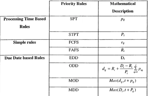
According to the previous studies, SPT and MOD rules are considered as the most effective rules for completion time and tardiness based criteria. Note that SPT and MOD are described as local rules. Conway and Maxwell (1962) define local priority rules as those that require infomiation only about those jobs that are waiting at a machine, while global rules require additional information about jobs or machine states or other machines. Shortest total processing time (STPT) and the modified job due date (MDD) rules can be considered as the global rules in this context. In this study we use these four rules. We believe that using local and global rules makes the results of the study more general and reliable. To seek more generality, we use two other local/global pairs of rules: ODD and FDD rules, which are again simple but effective rules. FCFS and FAFS lules are included as bench mark rules. Table 2.1 gives their mathematical definitions for the eight rules selected:

(31)

Table 2-1: Mathematical Description of Priority Rules Used in the Study

Priority Rules Mathematical

Description Processing Time Based

Rules

SPT P i j

SrPT P i

Simple rules FCFS _nj

FAFS R i

Due Date based Rules FDD D,

ODD

1 j v=i

MOD M a x ( d i j , t + Pij)

MDD M a x { D i , t + P i j )

Where:

i\ Index for job i j: Index for operation ,/

D ,: Due date of job i

dij: Due date of job i for operation / R i: Arrival time of job i at the system rij : Ready time of job i at operation / Pi'. Total operation time for job i

Pij·. Total remaining processing time for job i Pij‘. Processing time of job i at operation j

(32)

Chapter 3 System Considerations, Simulation model,

and Experimental Conditions

3.1 Suggested model

In a dynamic and stochastic manufacturing environment, testing scheduling rules under different experimental conditions becomes a more complex task than in the static case. It follows that we should be very careful on the model choice. The generality aspect of such a model tnust be kept at maximum in order to get potential benefits from the experiments.

Our model is similar to the one trsed by Vepsalainen and Morton (1987). It’s a reentrant dynamic job shop model with:

• Continuously available 10 machines

• Continuous arrival of jobs having a Poisson distribution

• Number of operations assigned to each job arrived is random having a uniform distribution U[l,10]

(33)

CHAPTER 3. System Considerations,... 15

• Each operation is equally likely to be performed on ten machines, where processing times are random having a uniform distribution U[1,30J.

3.2 Assumptions

The assumptions that would be considered in this model are typical ones found in most classical scheduling studies.

1. The model considered is a reenlrant job shop, (i.e. each job can get to the same machine twice a time if required).

2. Each operation can be performed by only one type of machines. 3. There is only one machine of each type in the shop

4. Processing times as well as due dates are known at the time of arrival of the job. 5. Set up times are sequence independent and can be included in the processing time. 6. Once an operation is begun on a maehine, it cannot be interrupted (i.e.,

preemption is not allowed).

7. An operation may not begin until its predecessors are complete 8. Each machine can process only one operation at a time.

9. Each machine is continuously available for production.

A point worth to note is tiuit the generality aspect of our model stems from the fact that we relax the assumption of deterministie job due dates. In this chapter, we assume that due dates can undergo variation during the job processing. In later chapters, we eonsider variation in the processing times and the system load level.

(34)

3.3 Experimental Conditions

3.3.1 Machine and Shop Utilization

The combined effects of job arrival distribution, Job routing and processing times determine the machine utilization. From the standpoint of job-shop simulation, machine utilization is important because it affects queue lengths. If the average queue length is too small, the scheduling rules used in the model may not be forced to make discriminating job selections; when this situation occurs, an evaluation of rule effectiveness is difficult or impossible. Adverse effects also result from machine utilization when it is too high. If the utilization is near 100%, transient conditions may extend over a long time period. Machine utilization commonly found in the literature ranges from 60% to 95%. This range of utilization permits scheduling rules to select a job from several in the queue but does not lead to very long queues.

In this paper, we will consider two levels of machine utilization: 60% (low) and 85% (high). We achieve the desiicd utilization level by adjusting the arrival rate.

3.3.2 Due Date Tightness

Due date performance of the rules are affected by due date tightness. In general, tighter due dates tend to produce larger values of MT (mean taidiness) and PT (proportion of tardy jobs), if othei conditions remain unchanged. Baker (1984). Beyond that there is also evidence (hat the relative performance of priority rules is also affected by due date tightness, at least for PT and for MT. This suggests the existence of so called cross over points, with one rule performing best for tighter due dates and another performing best for looser due dates. This cross over aspect is

(35)

CHAPTER 3. System Consideratious,... 17

somehow unwanted in tlie research area, that’s why we should be very careful in setting the tightness degree. In this study, based on the study done by Baker (1984), we propose an approach to determine the level of due date tightness in job shop systems. The approach assumes that if in two job shop systems, the assigned How allowances A/s to arriving jobs result in equal PT (proportion of tardy jobs) values, then the systems are undergoing similar due date tightness levels. Bakci' suggests that 10% and 40% PT values represent loose and relatively tight due dates respectively. These PT values are used as refeicnee values to apply due date tightness to the simulation experiments in this study.

3.3.3 Due Date Assignment Rule

Several different studies indicate thal shop performance and relative effectiveness of priority rules are affected by due dale assignment methods. In this study, we u.se the TWK approach in assigning the due dates. The reason is that TWK method is found to be the most efficient rule to reduce the cross over effect discussed in the previous section. According to TWK, job due dates are defined as follows:

Dj = Rj + Aj where,

Aj = k x Pj represents the original flow allowance, k is the due date tightness value,

and

Rj denotes the arrival time of job j.

In order to set tight due dales or loose due dates, the parameter k would be adjusted in order to achieve the required PT values mentioned previously (i.e. 10 % and 40% values). This depends on the priority rule used as well as on the machine

(36)

utilization level assigned. In fact, il’s worth noting that, a given value of k may achieve tight due dates in high machine utilization case but would lead to very loose due dates in low machine utilization ca.se. I hat’s why in this study, we use separate pilot runs to set values of k for diffeient machine utilization levels.

3.3.4 Performance Criteria

Several performance criteria have been u.sed to evaluate the scheduling rules. In the first part of this study we deal with two well known simple criteria, one is processing time based, the mean flow time (MF) and the other is due date based, the mean tardiness (MT). In a later stage, we introduce a non regular measure, the mean absolute deviation (MAD) criterion.

3.4 Model Implementation

The simulation models are developed using the SİMAN language (Pegden et al. 1995). The models are verified and validated with reference to the hypothetical model suggested previously. The validation process is done by checking that the outputs of the computer model are an accurate and valid representation of our hypothetical model. The common random number variance reduction technique (CRN) is implemented to compare the rules under identical conditions and to reduce the experimental error. Initially, some pilot runs are taken to find suitable values for the arrival rate to set the desired utilization levels. Two values are found for the arrival rate: 10.3 and 14.5 corresponding to 85% and 60% utilization levels, respectively. Furthermore, several other runs are also taken to estimate the warm up period using the Welch approach (Law and Kelton (1991)). As a result, 300 job completions are

(37)

deleted at the beginning of each run to reduce the effect of initial bias, hi order not to lose too much computer time, the batch means approach is used, ten batches are analyzed for each experiment run, with a batch size equals 900 for each one. Pilot runs are also taken to set the paramclcr k for each machine utilization level as shown in Table 3.1.

Note that the k values illusti aled in Table 3.1 are not appropriate with the due window approach, so other pilot runs are also taken to update k in the due window case. Results are illustrated in chapter 7.

Table 3-1: Due Date Tightness Parameter k Values

Tight due dates Loose due dates

High machine utilization (85%)

k = 4.5 k = 7

Low machine utilization (60%)

(38)

Chapter 4 Effect of Due Date Variation on the

Effectiveness of Priority Rules

4.1 Introduction

In real job shop environments, job due dates, though fixed before jobs go on process, may undergo changes after. This can be observed in real situations where due to some external or internal factors, manufacturers have to finish a job before or after its originally set due date. We expect that the variations that job due dates can undergo during the jobs processing, can have considerable negative impact on the performance of priority rules. Nevertheless, we are not aware of any study that considered tlie phenomenon. All studies in the literature assumed that due dates do not change once they are determined.

In this chapter, our objective is to investigate the effect of due date variation on the effectiveness of priority rules with MF and MT measure.

(39)

CHAPTER 4. Effect o f Due Date Variation ... 21

4.2 Modeling Due Date Variation

A job due date can be viewed in many dilTerent ways; it can be se( as a single point estimate that is determined by using some due date rule, or it can be set as an interval of time so-called due date window. In this chapter, we deal with the single point due dates approach. In chapter 7, we extend the study under the due window approach. The following describes the method of incorporating due date variation in our model.

As previously mentioned, 'I’WK method is used to set due dales in this study. In modeling this situation, each job is given a certain flow allowance once it enters the system. As the job moves from one machine to another, with a certain probability p, it will undergo a change in its actual due date. Practically, in real job shops, a job will have its due date either postponed or made more urgent. This will depend on two major factors or players, the first is the manufacturer side and the second is the customer side. Therefore, two scenarios can occur: First, if the job is expected to be late, or technically speaking, the job’s slack time is non positive, than the manufacturer may be obliged to ask the customer to agree on poslironing the job’s due date by a sufficient amount of time (at least equals its expected remaining manufacturing time). The next scenario occurs when the job is not to be late. In this case, the job’s slack time is positive. Consequently, the job due dale can be either postponed or made more urgent. This can occur in real situations wheie the customer needs the job to be finished eithei· less or more urgently. Consequently, the manufacturer may agree to change the job due date, within some limitations that the are set according to the actual status of the job. These two scenarios are defined as follows;

(40)

1) If its slack time at time t, Sf= clj -1 - Pj), where Pj is the remaining operation time) is positive then the actual due dale undergoes either a positive or negative change which equals DV*Sj, where DV is the due date variation coefficient (would range from 0.2 till 0.8 ).

2) Otherwise, the job due date is postponed by being added (1 + O.5*Z)V0*|*S'y|as a sufficient time to finish the job.

A point worth noting is that the experimental factors that would be controlled during the study are:

• The probability of undergoing due date change p: a small value 0.05 will initially be used and then this will be increased to 0.10 to see major effects of increasing the due date change rate.

• The due date variation coefficienl DV: this will range from 20%,40%,60% and 80%.

Of course, this approach could be more elaborated and improved, yet it will satisfy the goal of this study.

4.2.1 Due date variation analysis in terms of Mean Tardiness

The expression for MT performance measure is as follows: «

T-M T = 1 - ^

1=1 n

where.

Tj = Max{Cj - Dj,0) , Job,/ tardiness, Q: Completion time of job j

(41)

Once due date variation is included in the analysis, the M3’ perfonnancc of priority rules can change in teinis of two main components. The first is the completion time of each job, C/. Since the due date of some jobs change, their relative priority might change and consequently, completion times of jobs change. This effect due to changes in Q ’s is called Type-I ejfect. The second component is the due date

D j . Recall that the tardiness is a function of due dates. So, as the due dates of some

jobs change, their tardiness values in (urn change. 'I’liis effect is called Type-Il effect. The due date variation effect due (o suni of the.se two components determines the Overall effect on the M3’ performance of the priority rules.

In fact, it is important to differentiate between these three types of effects. Type-I effect measures the new pei lbrmance of the rule when it considers changes in due dates while assigning job prioi ilies during the dispatching process. That leads to new completion times of the jobs in (he process. But, the performance is measured in terms of the original due dates. In odier words, Type-I effect can l)c viewed as the net effect of due date variation on the dispatching policy perforniance. Note that non due date based rules are insensitive (o Type-1 effect as they do not consider any due date information.

On the other hand, 3’ype-ll effect gives the new performance of the rules when they disregard any change in job due dates during the dispatching process. But, their MT performance is measured in terms of the final due dates. A point to note is that non due date based rules are only sensitive to this type of effect, while due date based rules are affected by both effects. The overall effect is the conibination of the.se two effects and reflects the global effect of due date variation on the rule’s performance in terms of both changes in due date values and the dispatching policy performance.

(42)

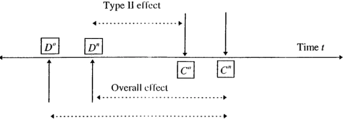
According to these three due date variation effects, Table 4.1 repre.sents the corresponding tardiness (7}) equations upon wliich the three elTects could be measured. We also present the rules .sensitive to such due date variation effects. A graphical illustration of these type elTccts is shown in Figure 4 .1.

Table 4-1; Corresponding 7} Equations to Due Date Variation Effect Types

Effect type Tj’s Equation Rules affected Rules not affected

Type I Tj=M ax{C; - Dj , 0 ) FDD, ODD, MOD, MDD

SPT, STPT, FCFS, FAFS

Type II Tj = Max(C; - D'! ,0) All rules None

Overall Tj = M ax(c; - d; ,o) All rules None

where,

CJ: Original (No due date variation) completion time of job./ D ": Original due date of job /

C" : New completion time of job ./ D'l: Final due date of job./

In fact, Type-II effect simply measures the due date variation .scheme that we adopt in terms due date value changes, which is not of much concern to the scope of the study. Consequently, only Type-1 and Overall effects will be measured throughout the simulation experiments.

(43)

Figure 4-1: Illustration of Type-I, 'I’ype-Il and Overall DV effects

Type 11 elTcct ■<... ► D' D" Time t C C" Overall cITect Type 1 effect

(44)

4.3 Analysis of the Simulation Results

The rules are tested under four levels of due date variation: 20%, 40%, 60% and 80%. Two performance measures, MF and MT are used to avoid bias. To seek generality, two system load levels 60% and 85% as well as two due date tightness levels (Tight and Loose) are considered. In order to investigate the effect of increasing the probability p of occurrence of due date changes, wc consider two p levels: 0.05 and 0.10. The simulalions results are illustrated in Tables A. 1-A. 12 (Appendix A). The pair t-tests are applied to compare the best rule with the next best rule at a significance level of 5%. The sign (*) indicates that the difference is significant. In addition, the pair /-tests are also used to compare the original performance (i.e. with no due date variation ) of a rule with its new performance when DV% level is increased. The sign (*·'■) indicates that the difference is significant. Furthermore, the rules performance versus due date variation graphs are plotted in Figures 4.2-4.19.

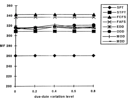
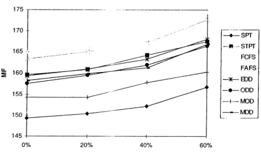
4.3.1 Mean Flow Time Criterion

Primarily, we should mention that non due date based rules such as SPT, STPT, FCFS and FAFS rules are insensitive to the due date variation factor. This is due to their primal nature that they do not consider any due date information. Consequently, as expected these rules produce the same MF performances with all five due date variation levels (Figure 4.2-4.5). According to these figures, we also observe that SPT always gives best MF values despite the DDV (due date variation) level, in all experimental conditions. This indicates that DDV do not affect the relative performance of SPT with other competing rules. Furthermore, we observe that FDD, ODD, MOD and MDD, although aie due date based rules, their performances are not

(45)

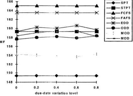
considerably affected by DDV in the liigli utilization case (Figures 4.2 and 4.3). In the low utilization case, we notice (hat their performance do not undergo regular deterioration, instead the performance of the rules fluctuates up and down (Figures 4.4 and 4.5). Nevertheless, the magnitude of up/down performance fluctuations is statistically insignificant (Table A.3 and A.4, Appendix A).

In summary, we conclude that the performances of priority rules are quite robust to DDV with respect to the MF measure. In addition, DDV do not have any significant impact on their relative performance. In particular, SPT is always the best performing rule despite any DDV level.

(46)

CHAPTER 4. Effect o f Due Date VaricUion ... 28

Figure 4-2: MF versus Due Date variation/ Exp. Coiul. 1

p = 0 .0 5 /H ig h u t ll iz a li on (l )5 % )/T lg h l d u c -d a te s (K = 4 . 5 )

Figure 4-3: MF versus Due Date variation/Exp. Concl. 2

(47)

Figure 4-4: MF versus Due Date variation/ Exp. Cond. 3

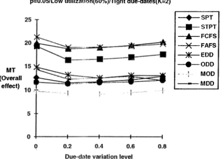
p = 0 . 0 5 / L o w u t ll lz a li o ? i (6 0 % )/ T ig h t d u e - d a t e s ( K = 2) --- S P T — STPT “A ---F C F S - X ---- FAF S - X — E DD - # ---O D D ! M O D --- M D D

Figure 4-5: MF versus Due Date variation/ Exp. Coiul. 4

(48)

4.3.2 Mean Tardiness Criterion

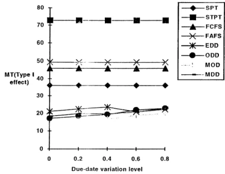
4.3.2.1 Analysis of Due Date Variation for 'rype-I Effect

The simulation results are tabulatetl in Tables A.4-A.8 in Appendix A. As expected, non due date based rules are insensitive to Type-I effect since these rules do not consider any due date information. On the other hand, due date ba.sed rules undergo an increasing deterioration pattern along the four DDV levels (Figures 4.6-4.13). This suggests that due date variation 'i’ypc-l effect can have negative impact on the MT performance of the rules.

As a matter of fact, the degree of this impact varies from one experimental condition to another. We observe (hat the slope of the deterioration curves is higher in the high machine utilization case (han in the low machine utilization case. This can be illustrated by comparing the slopes in Figures 4.6 and 4.10. Furthermore, if we compare the rules performances in (he p=0.05 case with the /7=0.10 case, we observe that the deterioration patterns become more severe for .almost all due date based rules (Figures 4.6 and 4.7). This indicates that DDV Type-I effect has more negative impact on the performance of the rules as either the probability at which due date changes occur or the machine utilization level is increased.

Furthermore, from Tables A.5-A.8 (Appendix A), we analyze the following behavior of some rules; global rules like MDD and FDD are more robust to Type-I effect than local rules like ODD and MOD. This is deduced by comparing the rates at which the rules performance is deteriorated as the DDV level is increased. For instance, according to Table A.5, we measure the magnitude of the MT performance

(49)

CHAPTER 4. Effect o f Due Dale Variation ... 31

Figure 4-6: M'l" ver.su.s l)I)V Type-I elTcc(/ Exp. Coiitl. I p=0.05/High utilizalion(85%)/Tight due-dates(K=4.5)

MT(Type effect) — FAFS e d d - # ----ODD : MOD MDD

Figure 4-7: MT versus DDV Type-I effeci/ Exp. Coiid. 2 p=0.10/Hlgh utllization(85%)/Tlght due-dates(K=4.5)

MT(Type effect)

(50)

Figure 4-8: MT versus l>I)V Type-I effect/ Exp. Cond. 3 p=0.05/High utilization(85%)/Loose due-dates(K=7)

SPT - B — STPT -j|r— FCFS FAFS - ^ E D D - ♦ — ODD -4 MOD MDD

Figure 4-9: MT versus l)I)V Type-1 effect/ Exp. Coiul. 4 p=0.10/High utilization(85%)/Loose due-dates(K=7)

(51)

CHAPTER 4. Effect o f Due Date Variation ... ₃₃

Figure 4-10: M F versus I)I)V Type-I effect/Exp. Coiid. 5 p=0.05/Low ulilizalion(60%)/Tighl due-dates(K=2)

- ♦ — SPT STPT - A — f c f s - X — FAFS - ^ E D D - ♦ — ODD ! MOD MDD

Figure 4-11: MT versus DDV Type-I effect/ Exp. Cond. 6 p=0.10/Low utilization(60%)/Tight due-dates(K=2)

(52)

Figure 4-12: MT versus DDV Type-1 effect/ Exp. Coiid. 7 p=0.05/low utilization(607o)/Loose due-dates(K=:3)

Figure 4-13: MT versus DDV Type-I effect/ Exp. Coiid. 8 p=0.10/Low utilization(607o)/Loose due-dates(K=3)

— EDO - ■ — ODD

MOD - X — MDD

(53)

deterioration from the DV=0% (o the DV=80% level. We find out that the performances of ODD and MOD’s performances worsens by 5.76 and 6.82 units respectively, whereas EDD and MDD’s performances worsens by only 1.14 and 4.46 units respectively. This suggests that a rule which utilizes global information (i.e., job due dates) instead of local information (i.e., operation due dates) arc more robust to the disturbances caused by the variation in due dates.

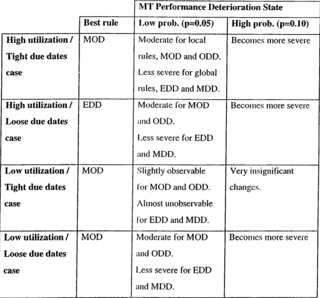
Based on the results obtained in this .section, we present a summary table (Table 4.2) which characterizes the effect of DDV on the priority rules for each experimental condition.

(54)

Table 4-2: Type-I effect / Summary of Results

MT Performance Deterioration State

Best rule 1 yow prob. (p=0.05) High prob. (p=0.10) High utilization /

Tight due dates case

MOD Moderate for local rules, MOD and ODD. Less severe for global rules, EDD and MDD.

Becomes more severe

High utilization / Loose due dates case

HDD Moderate for MOD and ODD.

Less severe for EDD and MDD.

Becomes more severe

Low utilization / Tight due dates case

MOD Slightly observable Ibr MOD and ODD. Almost unobservable Ibr EDD and MDD.

Very insignificant changes.

Low utilization / Loose due dates case

MOD Moderate for MOD and ODD.

Less severe for EDD and MDD.

(55)

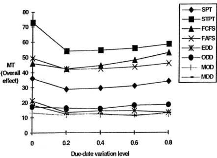
4.3.2.2 Analysis of Due Date Variation Overall Effect

The results of the simulation runs aic tabulated in Tables A.9-A.12 in Appendix A. After analyzing the performances ol the rules, we make the following observations:

Generally speaking, the performance of non due date based rules is negatively affected as we move from the DV=20% level to the DV=80% level. This can be observed in almost all experimental conditions (Figures 4.14-4.21), which concludes that the overall effect of DDV is to have a negative impact on the per formance of non due date based rules.

On the other hand, the performances of due date based rules, though impr ove at the DV=20% level, undergo almost no change as DDV increases beyond the 40% level (Figures 4.14-4.21). This indicates that due date based rules are quite robust to the overall effect of DDV. Note that MOD display best MT performance in almost all experimental conditions.

Even though the probability of DDV occurrence p is increased from 0.05 to 0.10, we observe no changes; due date based rules are still unaffected by DDV (see Figures 4.15,4.17,4.19,4.21)

In general, the relative pet formance of the priority rules is unaffected by DDV. Nevertheless, there are some exceptions. In the high utilization / loose due dates case, we observe a cross over between EDD and MDD (Table A. 10 Appendix A). At the DV=0% level, EDD displays best M'F performance, however, as we get beyond the 40% level, MDD displays the best MT values and outperforms EDD. Note that the differences between the performances of the two mles are statistically significant.

(56)

Figure 4-14: MT versus DDV Overall effect/ Exp. Coiid. 1 p=0.05/High utili2alioii(85%)night diie-dates(K=4.5)

- ♦ — SPT - a — STPT - A — FCFS - X — FAFS EDO - # — ODD I MOD — ^ M D D

Figure 4-15: MT versus DDV Overall effect/ Exp. Concl. 2 p=0.1cyH^i ulilizalioii(85yc)/TlÿTtKhje<la«es(IC=4.5)

(57)

Figure 4-16: MT versus ODV Overall effect/ Exp. Coiid. 3 p=0.05/High utilization(85%)/Loose due-dates(K=7)

Figure 4-17: MT versus DDV Overall efltct/ Exp. Coiid. 4 p=0.10/High utilizalion(857o)/l.oosc due-dates(K=7)

— SPT — B — STPT - A — f c f s — FAFS EDO - · — ODD [ MOD — — MDD

(58)

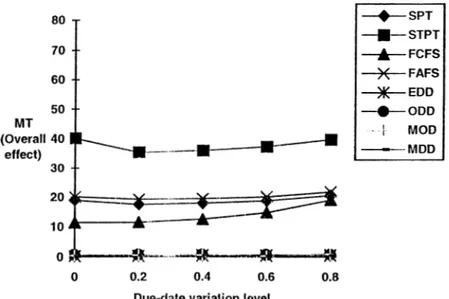
Figure 4-18: MT versus I)l)V Overall effect/ Exp. Coiul. 5 p=0.05/Low utilization(60%)/Tight due-dates(K=2)

MT (Overall effect) -SPT STPT — A — FCFS FAFS EDO ODD .... _MOD MDD

Figure 4-19: MT versus DDV Overall effect/ Exp. Cond. 6 p=0.10/Low utillzation(60%)/Tight due-dates(K=2)

MT (Overall effect) - 4 — SPT STPT - A — FCFS FAFS -^ E D D — ODD I MOD — — MDD

(59)

CHAPTER 4. Effect o f Due Date Variation ... ₄₁

Figure 4-20: MT versus DDV Overall effeci/ Exp. Coiul. 7 p=0.05/Low ulilization(60%)/Loose due-dates(K=3)

— SPT H i — STPT - A — f c f s - X — FAFS -^ E D D — ODD 4 MOD — MDD

Figure 4-21: MT versus DDV Overall effect/ Exp. Coiicl. 8 p=0.10/Low utilization(60%)/Loose due-dates(K=3)

— SPT - B — STPT - A — FCFS - X — FAFS ■^le— EDO - # — ODD I MOD — — MDD