Algorithms for 2 edge connectivity with fixed costs in telecommunications networks

(1)

ALGORITHMS FOR 2 EDGE

CONNECTIVITY WITH FIXED COSTS IN

TELECOMMUNICATIONS NETWORKS

a thesis

submitted to the department of industrial engineering

and the graduate school of engineering and science

of bilkent university

in partial fulfillment of the requirements

for the degree of

master of science

By

Umut G¨

uzel

(2)

I certify that I have read this thesis and that in my opinion it is fully adequate, in scope and in quality, as a thesis for the degree of Master of Science.

Assoc. Prof. Dr. Oya Kara¸san(Advisor)

Assoc. Prof. Dr. Hande Yaman

Assist. Prof. Ali Aydın Sel¸cuk

Approved for the Graduate School of Engineering and Science:

Prof. Dr. Levent Onural

Director of the Graduate School of Engineering and Science

(3)

ABSTRACT

ALGORITHMS FOR 2 EDGE CONNECTIVITY WITH

FIXED COSTS IN TELECOMMUNICATIONS

NETWORKS

Umut G¨uzel

M.S. in Industrial Engineering Supervisor: Assoc. Prof. Dr. Oya Kara¸san

July, 2011

In this thesis, several algorithms are developed in order to provide cost-effective and survivable communication in telecommunications networks. In its broadest sense, a survivable network is one which can maintain communication even in the presence of a physical breakdown. There are several ways of provid-ing survivable communication in a given network. Our choice is to hedge against single link failures and provide two edge disjoint paths for every source and desti-nation pair. Each edge in the network is assumed to have a variable unit routing cost and a fixed usage cost. Our objective is the minimization of the total routing cost of the traffic demand and the fixed cost of the utilized links. Several con-structive and improvement type heuristics are developed and tested extensively in an experimental design setting.

Keywords: 2 edge connectivity in telecommunications networks, Survivable net-woks, Primal and secondary paths .

(4)

¨

OZET

HABERLES

¸ME A ˘

GLARINDA SAB˙IT MAL˙IYETL˙I 2

AYRIT BA ˘

GLILIK ˙IC

¸ ˙IN ALGOR˙ITMALAR

Umut G¨uzel

Endüstri Mühendisli˘gi, Yüksek Lisans Tez Yöneticisi: Do¸c. Dr. Oya Kara¸san

Temmuz, 2011

Bu tez kapsamında, haberle¸sme a˘glarında uygun maliyetli ve güvenilir ileti¸sim sa˘glamak amacıyla ¸ce¸sitli algoritmalar tasarlanmı¸stır. En geni¸s tanım olarak güvenilir a˘glar, fiziksel bir arıza olu¸stu˘gunda bile ileti¸simi sürdürebilen a˘glardr. Haberle¸sme a˘glarında güvenilirli˘gi sa˘glamanın ¸ce¸sitli yolları vardır. Tek bir ayrıt arızasına kar¸sı önlem almak amacıyla her bir kaynak hedef ikilisi i¸cin 2-ayrıt yol buluyoruz. A˘gdaki her bir ayrıt rotalama maliyeti ve sabit maliyete sahip-tir. Amacımız kullanılan her bir ayrıtın sabit giderleri ve talep trafi¸gi rotalama maliyetleri toplamını enkü¸cültmektir. Ç e¸sitli sezgisel algoritmalar geli¸stirilmi¸s ve test edilmi¸stir.

Anahtar sözcükler : Haberle¸sme a˘glarında 2 ayrıt ba˘glılık, Güvenilir a˘g tasarımı, Birincil ve ikincil yollar.

(5)

v

(6)

Acknowledgement

I would like to express my sincere gratitude to both of my professors, Assoc. Prof. Dr. Oya Kara¸san and Assoc. Prof. Dr. Hande Yaman for their guidance, suggestions and supports during my graduate study.

I am indebted to Assist. Prof. Ali Aydın Sel¸cuk for accepting to read and review this thesis and also for his valuable time and comments.

I am grateful to T ÜB˙ITAK for their financial support during my research. I would like to thank to my family; my mother and father, Fatma Jale Güzel and Bahaddin Güzel and my brother Utku Güzel for their endless love and support throughout all my education life.

I would like to express my deepest gratitude to my beloved boyfriend Emre ˙Ilbars for giving me encouragement and motivation and also for his amazing patience and support.

I am most thankful to Aslı Deniz G¨uven and Utku C¸ ulha for their morale support and making this whole process endurable by their presence in the uni-versity.

Finally, I would like to thank to all my colleagues from Bilkent and friends for their support and friendship.

(7)

List of Figures

4.1 An example to show how Suurballe’s algorithm work . . . 20

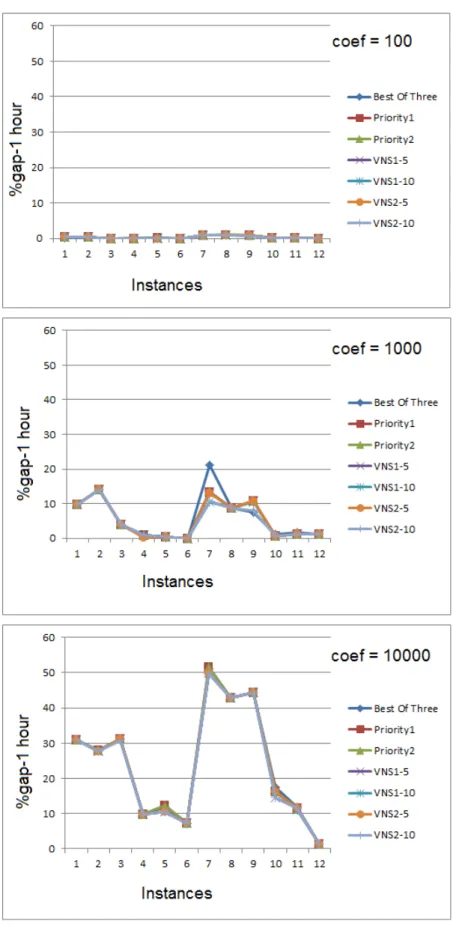
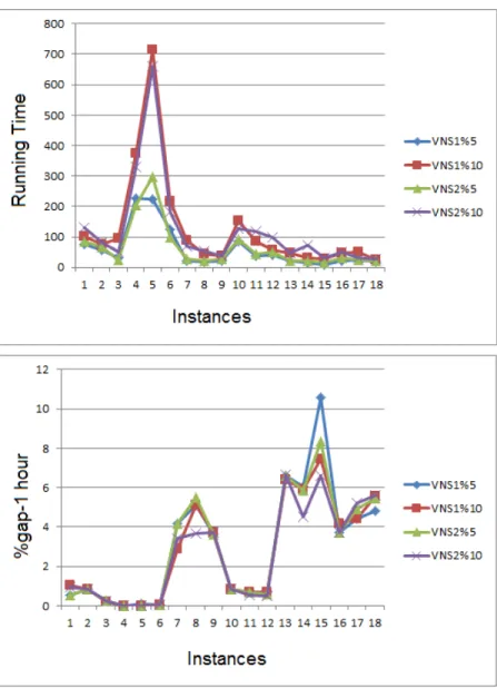
5.1 Instance-Gap Graphs for SPND Problem . . . 44 5.2 Instance-Gap Graphs for 2EDPND Problem . . . 47 5.3 Results of VNS algorithms for 2EDPND Problem for instances

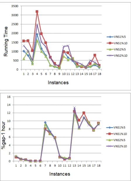
with |V | = 30 . . . 49 5.4 Results of VNS algorithms for 2EDPND Problem for instances

with |V | = 40 . . . 50

(11)

List of Tables

3.1 Notation . . . 13

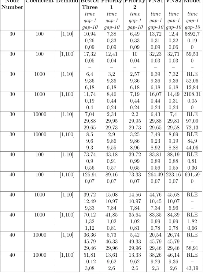
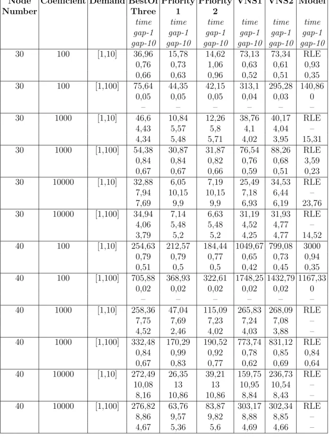
5.1 Average results for SPND Problem . . . 43 5.2 Average results for 2EDPND Problem . . . 46

A.1 Computational Results for SPND Problem with Node Number = 30 , Coefficient= 100, Demand ∈ {1,10} . . . 56 A.2 Computational Results for SPND Problem with Node Number =

30 , Coefficient= 100, Demand ∈ {1,100} . . . 57 A.3 Computational Results for SPND Problem with Node Number =

40 , Coefficient= 100, Demand ∈ {1,10} . . . 62 xi

(12)

LIST OF TABLES xii

A.8 Computational Results for SPND Problem with Node Number = 40 , Coefficient= 100, Demand ∈ {1,100} . . . 63 A.9 Computational Results for SPND Problem with Node Number =

40 , Coefficient= 10000, Demand ∈ {1,100} . . . 67 A.13 Computational Results for 2EDPND Problem with Node Number

= 30 , Coefficient= 100, Demand ∈ {1,10} . . . 68 A.14 Computational Results for 2EDPND Problem with Node Number

(13)

LIST OF TABLES xiii

A.20 Computational Results for 2EDPND Problem with Node Number = 40 , Coefficient= 100, Demand ∈ {1,100} . . . 75 A.21 Computational Results for 2EDPND Problem with Node Number

(14)

Chapter 1 Introduction

Networks are being used in many fields today. With the fast development of the Internet and broadened scope of communication, usage of networks has become wide spread and the requirements of the networks increased. A telecommunica-tions network consists of links and nodes. Links enable transferring data or signal between the nodes of the networks. Nodes can represent several different devices in a network such as switches or electrical devices. Links may represent wires, electrical cables, radio waves or optical fibers. There exist many different types of telecommunications networks and each one of them has different purposes. Tele-phone networks communicate in the form of sound, optical networks transfer data in the form of light, electrical networks transfer data in the form of electricity etc. Within the scope of this thesis is any one of these telecommunications networks where a survivable communication is essential.

Efficiency and reliability are the basic requirements in a network. In order to provide reliability, a network has to be capable of recovering failures and accidents that occur in nodes or links or any other device in the network. Networks have to be survivable to continue communication or data transfer in case of a failure. In a survivable network design there should exist more than one alternative way to provide communication; for example, there could be more than one path between a source and a destination pair. These additional paths are referred to as the recovery paths (secondary paths) for each communicating pair. Under normal

(15)

CHAPTER 1. INTRODUCTION 2

circumstances the primary or the initially designated path is used, but when a node or link failure occurs in the primary path of a pair, then the secondary path of this pair is used until the failure in the primary path is repaired. These paths need to be link or node disjoint. In this thesis, as is commonly done in the literature, it is assumed that only one failure can typically occur at a time in a network. Thus choosing edge or node disjoint paths between communication pairs will hedge against such breakdowns. In our thesis, edge disjointness will be adopted.

In the literature, survivability problem in networks is studied with different objectives like minimizing the total routing costs, minimizing the cost of the shorter path, minimizing the cost of the longer path or setting bounds for the costs of the paths. The objective of the problem might render the problem to be NP-hard. Furthermore, cost structure for the networks can also vary. In a network, cost for the primary path cp and the secondary path cs could be either

identical or different. If these two costs are different, there may be a relation between them as cs = αcp such that 0< α <1 or conversely these costs may be

arbitrary.

We are given a network G = (N, E, C, f ), in which N is the node set, E is the set of edges, C is the cost vector and f is the fixed cost vector. When an edge in E is used for the first time, a fixed cost is charged for installing that edge. However, if the same edge is used after it is installed, then only the routing cost for that edge is charged. Throughout the thesis, it is assumed that every possible node pair will communicate.

In this thesis we study two different problems; Fixed Charge Single Path Net-work Design Problem (SPND) and Fixed Charge 2 Edge-Disjoint Paths NetNet-work Design Problem (2EDPND). The first problem is to find a path for each com-municating pair, while minimizing the total cost. Total cost includes the fixed costs for the installed edges and the routing costs of the paths. This problem is studied by many different researches through the literature. It is known to be NP-hard. The second problem is to find 2 edge-disjoint paths for each source and target node pair, while minimizing the total cost. The first path is called as the

(16)

CHAPTER 1. INTRODUCTION 3

primary path and the second path is called as the secondary path. We consider different cost structures for the unit routing costs of the paths. Unit routing cost of an edge for the primary path is equal to the original cost of this edge. Since the secondary paths are less frequently used, only in case of failures, we assume that the unit routing cost of an edge is halved if it is used on secondary path. In our problem, the relationship between the path costs is cs = 1/2cp. This

prob-lem, which considers different cost structures, has been studied in the literature. However, most of these problems do not consider fixed costs. This problem is also NP-hard.

In order to solve the latter problem, we construct heuristic algorithms. First of all, we use a construction algorithm to find an initial solution for our problem. Then, we construct improvement heuristics to enhance the initial solution. Dif-ferent approaches are used while designing these improvement algorithms such as local search, variable neighborhood descent and variable neighborhood search. We also modified these algorithms to solve the former problem. Finally, these algorithms are tested and compared for both of the problems.

The remaining chapters of this thesis are organized as follows. Chapter 2 re-views the literature for the explained problems. Chapter 3 gives the mathematical models for the studied problems. In Chapter 4, construction and improvement heuristics are explained in detail. Chapter 5 states the computational analysis for the heuristics and mathematical models. In Chapter 6, thesis is summarized. In Appendix, tables of the numerical results can be found.

(17)

Chapter 2 Literature Review

Survivability has become a basic necessity for the network problems arising in telecommunications applications. In a survivable network, backup or recovery path must be available in addition to the primary path for each pair in case of a failure. If a failure occurs in a survivable network, that network will be able to recover itself. In normal circumstances primary path is used, but if a link or node failure happens in the primary path of a pair, then that pair will establish connection using the backup path. Since the backup path is used when the primary path becomes unserviced, these two paths must be edge or node disjoint.

We first focus on the problem of finding a single path for every possible node pair in a given network. If a single routing cost is used for each edge in the problem, then the problem is easy. It is enough to find the shortest paths to solve this problem. However, when fixed costs for each edge are considered the problem becomes more complicated. This problem is referred as the uncapaci-tated fixed charge network design problem in the literature. Literature review for uncapacitated fixed charge network design can be found in the first section.

Secondly, we work on the problem of finding two edge-disjoint paths for every potential source and target node pair in a given network G considering the routing costs and fixed costs, while minimizing the total cost. For this problem, unit

(18)

CHAPTER 2. LITERATURE REVIEW 5

routing cost of an edge for primary path is equal to the original cost of the edge and unit routing cost of the same edge for secondary path is equal to the half of the original cost of that edge. In both of the problems total cost includes routing cost of the paths for each commodity and sum of the fixed costs of utilized edges. When the literature is searched, it is seen that most of the problems in disjoint paths literature do not consider fixed costs. Literature review for disjoint paths can be found in the second section.

Both of the explained problems are NP-hard. Even though both problems are NP-hard, designing heuristic algorithms is more challenging for the second one. We have written a construction heuristic to find an initial feasible solution. But , finding an initial solution is not enough. In order to find better solutions, we construct several improvement algorithms which are applied to the initial solution. In the last section, literature review for heuristics can be found.

2.1 Uncapacitated Fixed Charge Network

De-sign Literature

Holmberg et al. [11] propose an exact algorithm to solve the problem of unca-pacitated fixed charge network design (UFCND). This algorithm uses Lagrangian heuristic with a branch and bound framework as a basis. This heuristic consists of three main parts; a construction heuristic to find a good initial solution, a subgradient search procedure and the Lagrangian relaxation of the problem.

Cruz et al. [5] also illustrates an exact algorithm which combines the branch and bound method and Lagrangian relaxation. They suggest a new technique to choose the branching variables for the branch and bound method.

Duhamel [7] states that UFCND is NP-hard. Duhamel illustrates two meta-heuristics to solve this problem. These metameta-heuristics are tested on the instances with up to 400 nodes and fixed cost of an edge is calculated as ten times the rout-ing cost. For smaller instances, optimal value is found. However as the instances

(19)

become larger running time increases, as a result the algorithm cannot approach to the optimal solution.

2.2 Disjoint Paths Literature

Through the literature, there exists several different versions of the problem of finding disjoint paths. Mainly, the objective functions of the problems are dif-ferent. Some problems aim to minimize the total cost whereas others aim to minimize the cost of a specific path. Furthermore, some problems search for edge disjointness, whereas the others search for node disjointness.

Damci [6] studies the problem of finding 2 edge disjoint paths between every possible source and target node in a given network. Additional to the routing costs, fixed costs for the edges are considered in this thesis. Objective is to mini-mize the total cost. Two construction algorithms and four different improvement methods are illustrated and tested for large number of instances. This problem is the same as our second problem, namely 2EDPND. We use the One-Step version 2 algorithm of Damci and we use the proposed improvement methods while we are constructing our improvement heuristics to solve our problem.

Suurballe [17] describes an algorithm to find k node-disjoint paths between a single pair of source and sink nodes, with minimum total length. The given algorithm finds the desired k paths at k iterations, at each iteration a single shortest path algorithm is used. As it is stated in [18], this algorithm can also be modified to find the k edge-disjoint paths. This modification of the algorithm is an O(m log_1+m/nn)-time algorithm and it uses O(m) space, where m is the number of edges and n is the number of nodes. For each pair, Suurballe and Tarjan [18] uses two iterations of Dijkstra’s single source algorithm. This algorithm solves the explained problem with optimality. In Suurballe’s problem, each edge is assigned only one cost whereas in our problem three different cost values are assigned to a single edge. For each edge {i, j}: unit routing cost for primary path is c1

ij, unit

(20)

Lee et al. [12] state an algorithm for the problem of finding k-best paths. It is the problem of finding k paths which are as different as possible and have the minimum cost in total. The algorithm described finds k paths which are both node-disjoint and edge-disjoint if there exist such paths, if not it finds k paths such that they are edge-disjoint and have minimum number of nodes in common. On the contrary, in our problem we want to find edge-disjoint paths between pairs. These paths can have common nodes since we have no restriction for node sharing.

Li et al. [13] consider the problem of finding k disjoint paths on a given graph G between s and t while minimizing the total cost of paths. This problem is different than those existing in the literature in that each edge has k different edge costs, where jth cost of an edge is related to the jth path. Four different versions of the stated problem are analyzed. Disjoint paths may be node or edge disjoint and the given graph may be directed or undirected. Li et al. show that all four variants of the problem is NP-complete even when k=2. They construct a polynomial time algorithm for the acyclic directed case and give heuristics for the proposed problem. In the heuristic algorithm, they average the costs on each edge and then solve a Minimum Cost Network Problem (MCNF). This study seems similar to our study, since they consider different edge costs for different paths. However, their costs have no relation, whereas we have a relation as: c2 _{= c}1_/2.

In addition, they do not consider fixed costs for the active edges.

Xu et al. [19] work on the problem of finding two disjoint paths such that the cost of the cheaper path is minimized. It is called the Min-Min problem. They proved that this problem is NP-complete. A heuristic is given for the Min-Min problem in which a divide-and-conquer technique is used. Different from the Min-Min problem, Min-Min-Max problem is also studied in [14] . Min-Min-Max problem aims to minimize the cost of the path which is more expensive than the other. Both of these problems are different from our problem in the sense of their objectives; our objective is to minimize the total cost which includes the costs of the primary and secondary paths for each commodity and plus the sum of the fixed costs of active edges.

(21)

Zheng et al. [20] discuss the problem of finding minimum-cost k paths sub-ject to defined minimum link/node sharibility constraints. Large node or link sharibility on a set of paths means, paths in this set have more nodes or links in common. If link/node sharibility for a path set is 0, then the paths in this set are link/node disjoint. The authors define five main sharibility constraints: min-sum node sharibility, min-min-sum link sharibility, min-max node sharibility, min-max link sharibility and the last one is having no restriction for the sharibility. They describe sixty five different constraints which are composite of the five main con-straints defined. An algorithm is given for the general problem. They proved that this problem for twenty five of the composite constraints are polynomially solv-able. This study is fundamentally different from ours, we want two paths to be only link-disjoint and we do not impose any restrictions on the node disjointness. Bhatia et al. [2] focus on the problem of finding a pair of disjoint paths of minimum total cost where cost of an edge for primary path is cij and cost of the

same edge for backup path is αcij, where α < 1. As a result, the contribution

of the cost of the backup path is smaller than the contribution of the cost of the primary path. They give an algorithm for the stated problem having an approximation ratio of O(1/α). This problem is very similar to ours, since in our problem α=1/2. However, as it is commonly done in the literature, the authors do not consider fixed costs for the activated edges. They state that if α is fixed, like in our study, NP-hardness of the problem is still an open question.

Gomes et al. [8] study the problem of finding k disjoint paths from a specified source node to target node, in a network such that each edge has k different cost values. Their objective is to minimize the total cost. They prove that, the proposed problem is NP-complete even when k=2. The authors give an exact algorithm to the problem of finding two arc disjoint paths for every node pair in a given network. This algorithm can be modified to find two node disjoint paths if desired. Similarly, with slight changes path lengths can also be bounded. The authors, work on the instances with at most 1000 nodes. Since each edge has k different cost values, this study is very similar to the problem discussed by Li et al. [13], which is previously stated. Our problem seems to be a special case of this problem for k=2, however each edge has two different costs in both problems, in

(22)

our problem these two costs have a relation between them whereas their costs are arbitrary. In addition, like the previous papers fixed costs of the edges are not considered.

Perl et al. [16] work on the problem of finding two disjoint paths P1 and P2

such that P1 is from s1to t1and P2is from s2 to t2. They consider four variants of

the problem; the given network can be directed or undirected, paths can be edge or node disjoint. They provide relations among these four different versions and construct efficient algorithms for some of the cases. This study is fundamentally different from our study, we find a pair of disjoint paths between a source and a target node whereas they find a pair of disjoint paths between two different pairs of nodes.

2.3 Heuristics Literature

Heuristic algorithms find good feasible solutions in reasonable computation times. We are interested in two different types of heuristics: construction heuristic and improvement heuristic. For a given problem, a construction heuristic finds an ini-tial feasible solution and an improvement heuristic starts from an iniini-tial solution and searches for a better solution. An example of an improvement heuristic is a local search algorithm. It starts with an initial solution and searches among a subset of solutions in a given neighborhood until the local optimum is found.

Sometimes local optima can be far away from the global optimal solution. In these cases meta-heuristics are needed. Metaheuristics are used when classic heuristics and combinatorial methods fail to solve complex optimization problems [15] . Metaheuristics have become an important application area through the last two decades. Metaheuristics aim to escape from the local optima found by local searches by for instance letting worsening solutions [3] .

Variable neighborhood search (VNS) basically uses the idea of the systemati-cal change of the neighborhoods as it is stated in [9] by Hansen et al. By the help of the neighborhood change VNS finds the local optima and then escapes from

(23)

the valleys that include these local optima. Hansen et al. explains the basic com-ponents of the Variable Neighborhood Search (VNS) and present some extensions of the VNS in their paper. Variable Neighborhood Descent (VND) is the basic version of VNS. VND algorithm starts with an initial solution as the current so-lution, assigns the first neighborhood as the current neighborhood and finds the best neighbor of the current solution in the current neighborhood. If the new solution is better than the current solution, current solution is updated and first neighborhood is assigned to the current neighborhood. If not, the next neighbor-hood is assigned as the current neighborneighbor-hood and the algorithm continues. VND terminates when no improvement exist.

Extensions of VNS are given such that: Reduced Variable Neighborhood Search (RVNS), Basic Variable Neighborhood Search (BVNS) and General Vari-able Neighborhood Search (GVNS). RVNS is very similar to the VND algorithm. The only difference is that, VND selects the best neighbor in the current neighbor-hood, whereas RVNS selects a random neighbor from the current neighborhood. BVNS, like RVNS generates a random neighbor in the current neighborhood but instead of comparing this point with the current solution, it applies a local search to the randomized point compare the new solution obtained from the local search with the current solution. GVNS starts with an existing solution x which is found by applying a local search to an initial solution found by a construction heuristic. After that, starting from the first neighborhood , a random solution is generated in the current neighborhood and VND is applied to this solution and obtain x0. If the cost of x0 is better than the cost of x, then x is updated as: x ← x0 and the algorithm continues with the first neighborhood. If not the next neighborhood is selected.

Variable neighborhood search algorithm is used to solve several different prob-lems in the literature. Br¨aysy [4] modifies the variable neighborhood descent algorithm to solve the problem of vehicle routing with time windows. Instead of using the original algorithm, a few changes are done. First of all, instead of finding the best neighbor, first neighbor in the current neighborhood is found. Furthermore, they changed the parameter values and objective function. The

(24)

algorithm changes the objective function to escape from the local optima. Hem-melmayer et al. [10] gives a new heuristic to solve the periodic routing problems without time windows. The authors use VNS as the underlying method of their heuristic.

In our improvement algorithms, we first use the idea of local search. Then we implement two different variants of Variable Neighborhood Search; Variable Neighborhood Descent and General Variable Neighborhood Search.

In the next chapter, our problems will be formalized and mathematical models will be provided.

(25)

Chapter 3 Mathematical Model

Development

In this chapter integer programs for the studied problems are given. We study two problems, the first one is the Fixed Charge Single Path Network Design Problem (SPND) and the second one is the Fixed Charge 2 Edge-Disjoint Paths Network Design Problem (2EDPND).

We are given a network G = (N, E, C, f ), where N is the node set, E is the edge set, C is the cost vector and f is the fixed cost vector. Both directions of a link can be utilized for communication. Thus, for the given network we create an arc set A as: {(i, j) ∪ (j, i) : {i, j} ∈ E}. Additionally, a commodity set K corresponding to a set of pairs of nodes in N is given. For each commodity k ∈ K, sk ∈ N is the source node, tk ∈ N is the destination node and dk ∈ Z+ is the

demand between source and destination. Each edge {i, j} ∈ E has two assigned costs, one is the unit routing cost Cij and the second one is the fixed cost fij,

which will be paid when an edge is used for the first time only. Notation can be seen at Table 3.1.

In the first problem, namely SPND, our aim is to find a single path for each commodity, while minimizing the total cost. Total cost consists of the fixed costs of active edges and the routing costs on the paths found for each commodity

(26)

CHAPTER 3. MATHEMATICAL MODEL DEVELOPMENT 13 Table 3.1: Notation G = (N, E, C, f ) : Given network N : Set of nodes in G E : Set of edges in G C : Cost vector of G f : Fixed cost vector of G K : Set of commodities in G

c1_ij : Unit routing cost for primary path of edge {i, j} ∈ E c2_ij : Unit routing cost for secondary path of edge {i, j} ∈ E sk: Source node of commodity k ∈ K

tk: Target node of commodity k ∈ K

dk : Demand of commodity k ∈ K

k ∈ K. Let Pk correspond to the single path for commodity k. For ease of

notation, we shall sometimes view Pk as the collection of edges or arcs on this

path. Cost of this path is calculated as follows, cost(Pk) =

P

{i,j}∈E∩PkdkCij.

Total cost is defined as: P

{i,j}∈E:(i,j) or (j,i) appears on some Pkfij +

P

k∈Kcost(Pk).

In the second problem, namely 2EDPND, our aim is to find two edge-disjoint paths for every commodity, while minimizing the total cost. Each edge in our network has two different routing costs; c1_ij is the unit routing cost for the pri-mary path c1

ij = Cij and c2ij is the unit routing cost for the secondary path c2ij =

Cij/2. Let Pk, Sk be the primary and secondary path for commodity k. cost(Pk)

= P

{i,j}∈E∩Pkdkc

1

ij and cost(Sk) = P{i,j}∈E∩Skdkc

2

ij. In this problem, the

to-tal cost consists of the fixed costs of active edges and the sum of routing costs of the two paths found for each commodity k ∈ K. Total cost is defined as: P

{i,j}∈E:(i,j) or (j,i) appears on some Pk or Skfij +

P

k∈Kcost(Pk) + cost(Sk).

3.1 Fixed Charge Single Path Network Design

Problem (SPND)

In this section mathematical model of the first problem will be provided. In the model two decision variables are used. Variables are as follows: binary variable xijk indicates the arcs utilized on the path of commodity k and binary variable

(27)

CHAPTER 3. MATHEMATICAL MODEL DEVELOPMENT 14

yij indicates the set of active edges.

xijk =         

1 if edge {i, j} ∈ E is used on the path of commodity k ∈ K in the direction from i to j

0 otherwise

yij =

 



1 if edge {i, j} is open 0 otherwise Model for SPND: min X {i,j}∈E fijyij + X k∈K X {i,j}∈E Cij(xijk+ xjik)dk (3.1.1) s.t. X j:(i,j)∈A xijk− X j:(j,i)∈A xjik =          1, if i = sk −1, if i = tk 0, otherwise ∀i ∈ N, ∀k ∈ K (3.1.2)

xijk+ xjik ≤ yij ∀{i, j} ∈ E, ∀k ∈ K

(3.1.3)

xijk ∈ {0, 1} ∀(i, j) ∈ E, ∀k ∈ K

(3.1.4)

yij ∈ {0, 1} ∀{i, j} ∈ E (3.1.5)

The objective function (3.1.1) consists of two parts; the first part is the sum-mation of the fixed costs of the activated edges and the second one is the summa-tion of the routing costs of a single path for each commodity k ∈ K. Constraint (3.1.2) is the flow balance constraint required for each commodity. Constraint (3.1.3) guarantees that if an edge {i, j} ∈ E is used on the path of a commodity, that edge is activated.

(28)

CHAPTER 3. MATHEMATICAL MODEL DEVELOPMENT 15

3.2 Fixed Charge 2 Edge-Disjoint Paths

Net-work Design Problem (2EDPND)

In this section mathematical model of the second problem will be provided. In the model three decision variables are used. Variables are as follows: binary variable xpijk indicates the arcs utilized on the primary path of commodity k, binary

variable xsijk indicates the arcs utilized on the secondary path of commodity k

and binary variable yij keeps track of active edges.

xpijk =         

1 if edge {i, j} ∈ E is used on the primary path of commodity k ∈ K in the direction from i to j

0 otherwise xsijk =         

1 if edge {i, j} ∈ E is used on the secondary path of commodity k ∈ K in the direction from i to j

0 otherwise

yij =

 



1 if edge {i, j} is open 0 otherwise

(29)

CHAPTER 3. MATHEMATICAL MODEL DEVELOPMENT 16 min X {i,j}∈E fijyij + X k∈K X {i,j}∈E

(c1_ij(xpijk+ xpjik) + c2ij(xsijk+ xsjik))dk (3.2.1)

s.t. X j:(i,j)∈A xpijk− X j:(j,i)∈A xpjik =          1, if i = sk −1, if i = tk 0, otherwise ∀i ∈ N, ∀k ∈ K (3.2.2) X j:(i,j)∈A xsijk− X j:(j,i)∈A xsjik =          1, if i = sk −1, if i = tk 0, otherwise ∀i ∈ N, ∀k ∈ K (3.2.3)

xpijk+ xsijk+ xpjik+ xsjik ≤ yij ∀{i, j} ∈ E, ∀k ∈ K

(3.2.4)

xpijk, xsijk∈ {0, 1} ∀(i, j) ∈ A, ∀k ∈ K

(3.2.5)

yij ∈ {0, 1} ∀{i, j} ∈ E

(3.2.6)

The objective function of the model (3.2.1) consists of two parts; the first part is the summation of the fixed costs of the active edges and the second one is the summation of the routing costs of both paths for each commodity k ∈ K. In the model there are two flow balance constraints (3.2.2) and (3.2.3). The first one is for the primary path and the second one is used for the secondary path for each commodity k ∈ K. Constraint (3.2.4) forces that an edge {i, j} ∈ E is used on at most one path;either primary or secondary for each commodity k ∈ K. It also ensures that if an edge {i, j} ∈ E is used on a path of a commodity, that edge is activated.

(30)

Chapter 4 Heuristic Algorithms

In this chapter, we detail our heuristic algorithms. These heuristics are designed to solve the problem of Fixed Charge 2 Edge-Disjoint Paths Network Design (2EDPND). Later on we modify these heuristics to be able to solve Fixed Charge Single Path Network Design(SPND) problem.

We use heuristics to get close to the optimal solution as much as we can. First of all, we obtain an initial feasible solution by a construction heuristic. Starting from this initial solution, several improvement heuristics using different methods are used to search and find better solutions. Improvement heuristics depend on three main heuristics, two of which are metaheuristics. As we know local search gets stuck at a local optimum. However, metaheuristics let algorithm to escape from the local optima. The first part of the improvement heuristics use the method of local search, the second part of the heuristics use the basic variable neighborhood descent and the last part of the heuristics use the general variable neighborhood search.

In our study, we have a network G=(N, E, C, f ) in which N denotes the node set, E denotes the edge set, C denotes the cost vector and f denotes the fixed cost vector. Each edge {i, j} ∈ E has a fixed cost fij in addition to a unit

routing cost Cij. The aim of our problem is to find, two edge disjoint paths for

every possible node pair, while minimizing the cost in total. A commodity set 17

(31)

CHAPTER 4. HEURISTIC ALGORITHMS 18

K is also given, which includes all possible node pairs as commodities. For each commodity k ∈ K, sk denotes the source node, tk denotes the destination node

and dk denotes the demand requested between source and destination nodes. We

shall use P as a path as well as the collection of edges or arcs present in P . As we have seen in the disjoint paths literature, for the problem of finding two edge disjoint paths between a single pair of source node s and destination node t, Suurballe’s algorithm [18] is a well known algorithm which solves the problem with optimality. This algorithm constitutes the basic idea of our heuristics.

In the first section, Route algorithm is illustrated. Route algorithm mainly uses Suurballe’s algorithm to find two edge-disjoint paths between the source and destination nodes of a given commodity k ∈ K. In the second section, RouteAll algorithm is given. RouteAll finds two edge disjoint paths for all commodities in K. Whenever the active edge set of a solution is updated, all commodities are rerouted using the RouteAll algorithm. In the third section, a construction algorithm is described which finds an initial feasible solution for the problem. Our construction algorithm is named as One-Step Algorithm. In the fourth section, our three main moves which are used in the improvement algorithms; adding an edge, deleting an edge and cycling an edge are defined. In the fifth section, improvement algorithms using the idea of local search are described. In the sixth section, improvement algorithms using the idea of basic variable neighborhood descent are illustrated. Finally in the last section, improvement algorithms using the idea of general variable neighborhood are explained.

4.1 Route Algorithm

Route algorithm finds two edge disjoint paths between two nodes of the given network, using the algorithm of Suurballe [18]. In Suurballe’s problem, each edge {i, j} ∈ E has only one routing cost Cij. The objective is to minimize the

total routing cost of these two paths. This algorithm is an O(m log_1+m/nn) -time algorithm and it uses O(m) space, where n is the number of nodes and m is the

(32)

number of edges. This algorithm is a modification of the algorithm given in [17], which finds two node-disjoint paths between a single pair.

Suurballe’s algorithm aims to find two edge disjoint paths between a source node s and a target node t. First of all, it finds the shortest path tree rooted at source node s using the Dijkstra’s algorithm [1], then constructs the first path to node t from this shortest path tree. Original cost for an edge {i, j} ∈ E is Cij

and shortest path distance from s to u ∈ N is denoted as dsu. Updated cost of

an edge {i, j} ∈ E is C_ij0 = Cij + dsi − dsj. Directions of the edges on the first

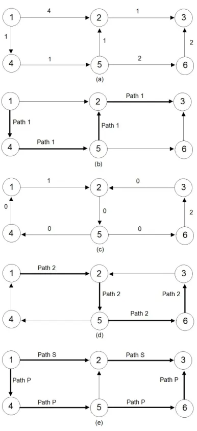
shortest path are reversed. The second shortest path is found between s and t using the updated costs and edge directions. Finally, the common edges in the first and second paths are discarded and two edge-disjoint paths from s to t are constructed. For a deeper understanding of this algorithm, Figure 4.1 can be analyzed. In this example our aim is to find 2 edge-disjoint paths between node 1 and node 3. Number on the edges are the edge costs. Part (a) of the figure shows the original network. In part (b), first path is constructed using the Dijkstra’ algorithm. Part (c) shows the transformed network. In part (d) using Dijkstra for the second time, the second path is constructed. Finally, after discarding the common edges, 2 edge disjoint paths are found between nodes 1 and 3. Path P represents the primary path and Path S represents the secondary path.

Route algorithm takes a network G0=(N0, E0, C0), in which N0 denotes the node set, E0 denotes the edge set, C0 denotes the cost vector and a commodity k as an input and finds two edge-disjoint paths from sk to tk in G

0

. First of all, a directed graph has been constructed from G0. An arc set −→E is defined for the directed graph. For each edge {i, j} ∈ E0, arcs (i, j) and (j, i) ∈ −→E . Costs of arcs (i, j) and (j, i) are equal to C_ij0 . It finds the paths using the Suurballe’s algorithm and assigns the path with the smaller cost as the primary path and the path with the larger cost as the secondary path and calculates the total cost for the commodity k. This algorithm outputs the primary and secondary path and the cost for the given commodity k: Pk, Sk and costk. The pseudo code of Route

(33)

(34)

Algorithm 1 Route

INPUT: a network G0=(N0,E0,C0, f ) , a commodity k OUTPUT: primary path P, secondary path S, cost Let −→E = {(i, j) ∪ (j, i) : {i, j} ∈ E0} , −→Cij ₌

−→ Cij _{= C}0 ij ∀{i, j} ∈ E 0 and − → G =(N ,−→E ,−→C )

Compute a shortest path tree rooted at node sk in graph

− →

G using Dijkstra’s algorithm.

Let P denote a shortest path from node sk to node tk.

Let dsku denote the shortest path distance from node sk to node u.

Let G−→0 = ( N0, −E→0 ,C−→0 ) where −→E0 is the same as −→E except that the directions of arcs on path P are reversed and ∀ (i,j) in −E→0: −→C0ij =

− →

Cij + dski - dskj

Compute a shortest path P0 from node sk to node tk in

− →

G0 using Dijkstra’s algorithm.

if one or more links appear in both P and P0 (in opposite direction) then Discard these links.

Construct 2 edge disjoint paths from sk to tk using remaining links.

Let P ← path with the smaller cost Let S ← path with the larger cost cost = (P

(35)

4.2 RouteAll Algorithm

RouteAll algorithm constructs two edge-disjoint paths for each commodity k ∈ K. This algorithm takes a network G0 as an input and using the Route algorithm k times, it finds two edge-disjoint paths between sk and tk for every commodity

k ∈ K in G0. It returns the solution found as an output. For a solution X, X_A− denotes the set of active edges, X_R denotes the routing set, which includes

two paths Pk and Sk for all k ∈ K, Xw denotes the weight matrix which keeps

track of the demand carried by each edge {i, j} ∈ E and Xtotalcost denotes the

total cost. In order to know the amount of demand that is carried by a single edge, weight of that edge is calculated for every edge {i, j} ∈ E. Weight of an edge {i, j} in a solution X is denoted as Xw

ij and equals to

P

k∈K:{i,j}∈Pkdk +

P

k∈K:{i,j}∈Skdk/2. Weight of an edge is used in two different steps; in one step

algorithm to distribute fixed cost of the edges and in cycle move. T otalcost of a solution X is calculated as: P

k∈Kcostk +

P

{i,j}∈X_A−fij. The first part is the

sum of the costs of the commodities, and the second part is the sum of the fixed costs of the active edges. Pseudo code of the given algorithm can be seen in Algorithm 2. Algorithm 2 RouteAll INPUT: a network G0=(N0,E0,C0, f ) OUTPUT: a solution X XA− ← ∅ XR← ∅ for all k in K do

Route(G0, k ) and get Pk, Sk, costk

Add paths Pk and Sk to set XR

XA− ← X_A−∪ P_k∪ S_k

X_ijw=P

k∈K:{i,j}∈Pkdk+

P

k∈K:{i,j}∈Skdk/2 for all {i, j} ∈ XA−

Xtotalcost =

P

k∈Kcostk +

P

(36)

4.3 One-Step Algorithm

One-Step algorithm is a construction heuristic, which is used to find an initial feasible solution for our problem. In One-Step algorithm, all commodities in K are routed three different times using Suurballe’s algorithm. Since Suurballe uses a single routing cost for each edge {i, j} ∈ E, while solving our problem it is important to decide which cost structure to use for edges.

As an initial step, a routing is done with only using the original routing costs of the edges C, without considering the fixed costs. Each commodity k ∈ K is considered separately in this case. Then, the set K is sorted in the descending order of costs of commodities and second application of the routing is done in this order. Assume, solution X is obtained from the first routing.

In the second application, we use the fixed costs of the edges additional to their original unit routing costs. We force algorithm to consider fixed costs of the edges when assigning the paths. For the solution X, which is found at the end of first application, we calculate a weight X_ijw for each edge {i, j} ∈ E. We use weight to distribute the fixed costs of the edges. Before applying RouteAll, we update cost of each edge {i, j} ∈ E as Cij + fij/Xijw. During the second

application, after each commodity is routed, cost of {i, j} ∈ E which have been activated is updated as Cij. At the end of this application, we obtain a new

solution X.

In the third and last application of RouteAll, original unit routing costs are used. This time we use only the activate edges in XA−. The logic behind applying

the RouteAll algorithm for the third time is to close the unused edges. At the end of this algorithm, an initial feasible solution X is returned. Pseudo code of One-Step algorithm can be found in Algorithm 3.

(37)

Algorithm 3 One-Step

INPUT: original network G=(N ,E,C,f ) OUTPUT: an initial solution X

RouteAll(G) and get solution X

Sort the set K in descending order of costk

C_ij0 ← Cij + fij/Xijw for all {i, j} ∈ E

Let G0 = ( N ,E ,C0 ) Define a new solution X0 X_A0− ← ∅

for all k ∈ K do

Route(G0, k ) and get Pk, Sk, costk

X_A0− ← X 0

A−∪ Pk∪ Sk

C_i,j0 ← Ci,j for all {i, j} ∈ (Pk∪ Sk)

Let G− = ( N ,X_A0− ,C )

RouteAll(G−) and get solution X

4.4 Moves

Until now, we only focused on constructing an initial feasible solution. From this point on we are interested in improving the initial solution. Our aim is to find a better solution than the initial one. As we explained before, each solution has a set of active edges. Two main modifications can be done in the active edge set. The first one is activating an inactive edge; rerouting with the new active edge set leads us to a new solution. Since, we activate a new edge, some previous edges can become unused and as a result of this, the new solution can have a smaller total cost than the previous one. On the other hand, if none of the previous edges becomes inactive, total cost can be larger than the previous one. The second one is inactivating an active edge in this set; rerouting with the new active edge set leads us to a new solution. This solution may be infeasible. If the new solution is feasible, then the cost of the new solution is compared with the current one. It can be either smaller or larger.

We define three different moves considering these two main modifications. These moves are as follows: Add Edge, Delete Edge and Cycle Edge. They will be used inside the improvement algorithms. Cycle Edge uses the idea of both Add

(38)

Edge and Delete Edge. For a solution X, for each move, an edge set is defined as XM ovename which includes the potential edges which lead feasible solutions when

this move is applied to X.

4.4.1 Add Edge

For every solution X, XAddis defined. XAdd includes all the inactive edges in the

solution X. Add Edge move takes an inactive edge {i, j} ∈ XAdd and a solution

X as input. The given edge is activated and added to the set of active edges of the given solution. All commodities are rerouted using the new set of active edges and original routing costs, at the end a new solution is found. Pseudo code of Add move can be seen in Algorithm 4.

Algorithm 4 Add Edge

INPUT: {i, j} and a solution X OUTPUT: a solution X

Let G− = ( N , (XA−∪ {i, j}), C )

RouteAll (G−) and get solution X

4.4.2 Delete Edge

This move is the opposite of the previous one. For every solution X, XDelete

is defined. XDelete includes all the active edges in the solution X such that

inactivation of that edge leads to a feasible solution. Delete Edge move takes an active edge {i, j} ∈ XDelete and a solution X as input. The given edge is

inactivated, i.e., removed from the set of active edges of the given solution. All commodities are rerouted using the new set of active edges and original routing costs, at the end a new solution is found. Pseudo code of this move can be seen in Algorithm 5.

(39)

Algorithm 5 Delete Edge

INPUT: {i, j} and a solution X OUTPUT: a solution X

Let G− = ( N , (XA−\ {i, j}), C )

4.4.3 Cycle Edge

We construct a move which includes the two main modifications: adding an edge and deleting an edge. This move is the composition of the previous two moves. In this move an edge is inactivated while several edges are being activated. This move also takes an active edge and a solution X as input. This move has a main difference from the previous ones, it considers the fixed costs. Assume we are cycling the edge {i, j} ∈ E. First of all, cost vector is updated such that if an edge {k, l} ∈ E is in the set of active edges of X its cost is Ckl, if not its cost

is Ckl+ (fkl/Xijw). For the given edge, a third path which has no common edges

with the primary path and the secondary path is found using Dijkstra with the updated cost vector, if it exists. For every solution X, XCycle is defined. XCycle

includes all the active edges in the solution X such that a third path can be found as it is described. The given active edge is inactivated, while the edges on the third path are activated and added to the set of active edges. All commodities are rerouted using the new set of active edges and original routing costs, at the end a new solution is found. Pseudo code of this move can be seen in Algorithm 6.

4.5 Improvement Heuristics: Local Search

In this part, improvement algorithms, which use the idea of local search, are presented. All of these algorithms are applied after running the One-Step con-struction heuristic. An initial feasible solution is found at the end of One-Step algorithm. These algorithms start from this initial solution as a current solu-tion and search for new solusolu-tions. When new solusolu-tions are found with improved

(40)

Algorithm 6 Cycle Edge

INPUT: {i, j} and a solution X OUTPUT: a solution X for all {k, l} ∈ E do if {k, l} ∈ A− then C_kl0 ← Ckl else C_kl0 ← Ckl+ fkl/Xijw

Temporarily delete the edges used in primary and secondary paths of {i, j} pair and find a new shortest path P= from i to j using Dijkstra’s algorithm with the cost vector C0

Let G− = ( N , (XA−\ {i, j} ∪ P=), C )

costs, the current solution is updated. All improvement algorithms take the ini-tial solution found by One Step algorithm as an input and output the current solution when the algorithm terminates. Local search heuristic, searches a given neighborhood of the initial solution. It stops at a local optima.

4.5.1 First Selection Algorithms

There exist three different versions of this algorithm, corresponding to the three different moves described above. These algorithms assign the initial so-lution as the current soso-lution. In these algorithms, for the selected move M ∈ {Add, Delete, Cycle} each edge {i, j} ∈ XM is selected one by one, move

M is applied to X and new solutions are obtained. Among these new solutions, the first improving solution is selected and assigned as the current solution. This algorithm continues until none of the possible edges improve the current solu-tion. Pseudo codes of the three different versions of the algorithm can be seen in Algorithms 7,8 and 9.

(41)

Algorithm 7 Add First

INPUT: a solution X obtained from One-Step Algorithm OUTPUT: a solution X0

Let X0 be the current solution X0 ← X

repeat

Find an edge {i, j} ∈ X_Add0 that Add Edge ({i, j}, X0) returns a solution X such that Xtotalcost < X

0

totalcost

Update X0: X0 ← X

until there does not exist such an edge {i, j}

Algorithm 8 Delete First

repeat

Find an edge {i, j} ∈ X_Delete0 that Delete Edge ({i, j}, X0) returns a solution X such that Xtotalcost < X

0

totalcost

Update X0: X0 ← X

until there does not exist such an edge {i, j}

Algorithm 9 Cycle First

repeat

Find an edge {i, j} ∈ X_Cycle0 that Cycle Edge ({i, j}, X0) returns a solution X such that Xtotalcost < X

0

totalcost

Update X0: X0 ← X

(42)

4.5.2 Best Selection Algorithms

There exist also three different versions of this algorithm, corresponding to the three different moves described above. In these algorithms, for the selected move M ∈ {Add, Delete, Cycle} each edge {i, j} ∈ XM is selected, move M is

ap-plied one by one to X and new solutions are obtained. The solution for the edge {i, j} ∈ XM, that has the smallest total cost is selected and if it improves the

current solution, it is assigned as the current solution, if not the algorithm termi-nates. Pseudo codes of the three different versions of the algorithm can be seen in Algorithms 10,11 and 12.

Algorithm 10 Add Best

repeat

Find an edge {i, j} ∈ X_Add0 such that Add Edge ({i, j}, X0) returns a solution X with the smallest cost

if cost is improved then Update X0: X0 ← X until cost is not improved Algorithm 11 Delete Best

repeat

Find an edge {i, j} ∈ X_Delete0 such that Delete Edge ({i, j}, X0) returns a solution X with the smallest cost

if cost is improved then Update X0: X0 ← X until cost is not improved

(43)

Algorithm 12 Cycle Best

repeat

Find an edge {i, j} ∈ X_Cycle0 such that Cycle Edge ({i, j}, X0) returns a solution X with the smallest cost

if cost is improved then Update X0: X0 ← X until cost is not improved

4.5.3 Best Of Three

In this algorithm our aim is to select the most improving solution found among the best selections of the three moves: Add, Cycle and Delete for a current solution. As an initial step, Best Of Three takes the initial solution as the current solution X. Then for the current solution checks for the edge {i, j} ∈ XAddwhich has the

solution X with the smallest total cost, checks for the edge {i, j} ∈ XDelete which

has the solution X with the smallest total cost and lastly checks for the edge {i, j} ∈ XCycle which has the solution X with the smallest total cost. Among

these three edges, the one finds the solution with the smallest total cost is selected and if it improves the current cost, then the current solution is updated. If not, the algorithm terminates. Pseudo code of this algorithm can be seen in Algorithm 13.

4.6 Improvement Heuristics:

Basic Variable

Neighborhood Descent(VND)

In this section, improvement algorithms, which use the idea of the basic variable neighborhood search, are described. All of these algorithms are applied after running the One-Step construction heuristic. Both of these algorithms take the initial solution found by One Step algorithm as an input and output the current

(44)

Algorithm 13 Best Of Three

f lag ← true f ound ← f alse

Let X0 be the current solution and X” be the temporary solution X0 ← X

while flag do X0 ← X

Find an edge {i, j} ∈ X_Add0 that Add Edge ({i, j}, X0) returns a solution X with the smallest cost

if Xtotalcost < Xtotalcost” then

Update X”_{: X}” _{← X}

f ound ← true

Find an edge {i, j} ∈ X_Delete0 that Delete Edge ({i, j}, X0) returns a solution X with the smallest cost

Update X”: X” ← X f ound ← true

Find an edge {i, j} ∈ X_Cycle0 that Cycle Edge ({i, j}, X0) returns a solution X with the smallest cost

Update X”_{: X}” _{← X} f ound ← true if found then Update X0: X0 ← X else f lag ← f alse

(45)

solution when the algorithm terminates. Variable neighborhood descent assigns the first neighborhood as the current neighborhood and finds the best neighbor of the current solution in the current neighborhood. If the new solution is better than the current solution, current solution is updated and first neighborhood is assigned as the current neighborhood. If not, the next neighborhood is assigned as the current neighborhood and the algorithm continues. VND terminates when no improvement exist. We have to order the three moves as the neighborhoods. Since Cycle Edge move includes the other two moves, we assigned it as the first neighborhood.

4.6.1 Priority1

The neighborhoods are ordered as: Cycle Edge, Delete Edge, Add Edge. As an initial step, Priority1 takes the initial solution as the current solution X. As the first step, for the solution X it finds the edge {i, j} ∈ XCycle which returns the

solution X0 with the smallest total cost. If it improves the current cost, then algorithm updates the current solution and repeats previous step until the cost is not improved. If current cost is not improved, finds the edge {i, j} ∈ XDelete

which returns the solution X0 with the smallest total cost. If it improves the current cost, the algorithm updates the current solution and goes back to the first step. If cost is not improved, finds the edge {i, j} ∈ XAdd which returns

the solution X0 with the smallest total cost. If it improves the current cost, the algorithm updates the current solution and goes back to the first step. If cost is not improved, the algorithm terminates. Pseudo code of this algorithm can be found in Algorithm 14.

4.6.2 Priority2

This algorithm is very similar to the previous one. The only difference is the order of the neighborhoods. The new order of the neighborhoods is: Cycle Edge, Add Edge, Delete Edge. Pseudo code of this algorithm can be found in Algorithm 15.

(46)

Algorithm 14 Priority1

f lag ← true

while flag do

if cost is improved then Update X0: X0 ← X else

(47)

Algorithm 15 Priority2

f lag ← true

while flag do

(48)

4.7 Improvement Heuristics: General Variable

Neighborhood Descent

In this section, improvement algorithms, which use the idea of the general variable neighborhood search, are explained. All of these algorithms are applied after running the One-Step construction heuristic. Both of these algorithms take the initial solution found by One Step algorithm as an input and output the current solution when the algorithm terminates. General VNS starts with a current solution X which is found by applying a local search to an initial solution After that, starting from the first neighborhood , a random solution is generated in the current neighborhood and VND is applied to this solution and obtain X0. If the cost of X0 is better than the cost of X, then X is updated as: X ← X0 and the algorithm continues with the first neighborhood. If not the next neighborhood is selected. Priority1 is used as the VND algorithm that is used in GVNS. We define a limitation for the number of edges randomly selected at each step of the algorithm, which is denoted as N I, to have a termination condition. This limitation is calculated as a percentage of the number of active edges for the solution X found by the algorithm Priority1. N I is equal to |XA−|α. We assign

two different values to α: 0,05 and 0,1. The following two algorithms have only one difference, it is the logic of the neighborhood change.

4.7.1 VNS1

One Step algorithm is performed and an initial solution is obtained. Then, the algorithm Priority1 is applied to the initial solution and solution X is obtained. In this algorithm, there exists three main phases. In the first phase our neigh-borhood is the cycle move. The algorithm selects an edge randomly from the set of XCycle. Cycle that edge and get a new solution, then apply Priority1 to the

new solution. If the current solution is improved, update the current solution and try N I random edges for the new solution. If not, select a new random edge from the set XCycle. When N I random edges are tried and current solution is not

(49)

neighborhood is the add move. The algorithm selects an edge randomly from the set of XAdd. Add that edge and get a new solution, then apply Priority1 to the

new solution. If the current solution is improved, update the current solution and go back to the first phase. If not, select a new random edge from the set XAdd.

When N I random edges are tried and current solution is not improved, then the algorithm passes to the third phase. In the third phase our neighborhood is the delete move. The algorithm selects an edge randomly from the set of XDelete.

Delete that edge and get a new solution, then apply Priority1 to the new solu-tion. If the current solution is improved, update the current solution and go back to the first phase. If not, select a new random edge from the set XDelete. When

N I random edges are tried and current solution is not improved, the algorithm terminates. Pseudo code of this algorithm can be seen in Algorithm 16.

4.7.2 VNS2

VNS2 is very similar to the previous algorithm. The only difference is the logic behind the neighborhood change. The neighborhood for the first phase is the same; cycle. But when we pass to the second phase this time we enlarge the neighborhood set. Neighborhood set includes both cycle and add. The algorithm selects one of them randomly. When the algorithm starts to third phase, the neighborhood set is enlarged one more time. This time neighborhood set includes cycle, add and delete. The algorithm selects one of them randomly. Pseudo code of this algorithm is given in Algorithm 17.

(50)

Algorithm 16 VNS1

Let X00 be the current solution,

Priority v1(X) and get the solution X0, X00 ← X0 N I ← d| (X_A00−) | ∗αe

f lag ← true while flag do

index ← 0, f ound ← f alse while index < N I do

Randomly select an edge {i, j} ∈ X_Cycle00 ,Cycle Edge({i, j}, X00) and get X Priority v1(X) and get the solution X0

if X_totalcost0 < X_totalcost00 then X00 ← X0

index ← 0 else

index ← index+1 index ← 0

while (f ound == f alse AND index < N I) do

Randomly select an edge {i, j} ∈ X_Add00 ,Add Edge({i, j}, X00) and get X Priority v1(X) and get the solution X0

if X_totalcost0 < X_totalcost00 then X00 ← X0

f ound ← true else

Randomly select an edge {i, j} ∈ X_Delete00 ,Delete Edge({i, j}, X00) and get X

Priority v1(X) and get the solution X0 if X_totalcost0 < X_totalcost00 then

X00 ← X0 f ound ← true else index ← index+1 if index==NI then f lag ← f alse

(51)

Algorithm 17 VNS2

Let X00 be the current solution, X00 ← X

Priority v1(X) and get the solution X0, X00 ← X0 N I ← d| (X_A00−) | ∗αe

f lag ← true while flag do

index ← 0, f ound ← f alse while index < N I do

Randomly select an edge {i, j} ∈ X_Cycle00 ,Cycle Edge({i, j}, X00) and get X Priority v1(X) and get the solution X0

if X_totalcost0 < X_totalcost00 then X00 ← X0, index ← 0 else

while (f ound == f alse AND index < N I) do Randomly select an edge {i, j} ∈ (X_Cycle00 ∪ X_Add00 ) if {i, j} ∈ X_Cycle00 then

Cycle Edge({i, j}, X00) and get the solution X else

Add Edge({i, j}, X00) and get the solution X Priority v1(X) and get the solution X0

if X_totalcost0 < X_totalcost00 then X00 ← X0, f ound ← true else

Randomly select an edge {i, j} ∈ (X_Cycle00 ∪ X_Add00 ∪ X_Delete00 ) if {i, j} ∈ X_Cycle00 then

Cycle Edge({i, j}, X00) and get the solution X else

if {i, j} ∈ X_Add00 then

Add Edge({i, j}, X00) and get the solution X else

Delete Edge({i, j}, X00) and get the solution X Priority v1(X) and get the solution X0

if X_totalcost0 < X_totalcost00 then X00 ← X0, f ound ← true else

index ← index+1 if index==NI then

(52)

Chapter 5 Computational Results

In this chapter, construction and improvement algorithms, which are explained in the previous chapter are tested in a computer with 1.73 GHz Core i7 740 processor and 4 GB of RAM. In order to find the optimal solution for the instances, the mathematical model described in Chapter 4 are solved using GAMS 22.3 and CPLEX 10.1.0.

5.1 Test Instances

In this section construction of the test instances are explained.

The number of nodes (|N |) for the test instances is either 30 or 40. We could not take node number larger, because even when |N | = 40 in some instances our mathematical model runs out of memory. In such cases, when we do not have the optimal solution at hand, we use the lower bound obtained from the model to calculate %gap.

We have three different probability values p= 1, 0.75, 0.5. Edges in the network are generated randomly with a probability p. When p = 1, the network is complete.

Algorithms for 2 edge connectivity with fixed costs in telecommunications networks

ALGORITHMS FOR 2 EDGE

CONNECTIVITY WITH FIXED COSTS IN

TELECOMMUNICATIONS NETWORKS

a thesis

submitted to the department of industrial engineering

and the graduate school of engineering and science

of bilkent university

in partial fulfillment of the requirements

for the degree of

master of science

By

Umut G¨

uzel

ABSTRACT

ALGORITHMS FOR 2 EDGE CONNECTIVITY WITH

FIXED COSTS IN TELECOMMUNICATIONS

NETWORKS

¨

OZET

HABERLES

¸ME A ˘

GLARINDA SAB˙IT MAL˙IYETL˙I 2

AYRIT BA ˘

GLILIK ˙IC

¸ ˙IN ALGOR˙ITMALAR

Acknowledgement

Contents

List of Figures

List of Tables

Chapter 1

Introduction

Chapter 2

Literature Review

2.1

Uncapacitated Fixed Charge Network

De-sign Literature

2.2

Disjoint Paths Literature

2.3

Heuristics Literature

Chapter 3

Mathematical Model

Development

3.1

Fixed Charge Single Path Network Design

Problem (SPND)

3.2

Fixed Charge 2 Edge-Disjoint Paths

Net-work Design Problem (2EDPND)

Chapter 4

Heuristic Algorithms

4.1

Route Algorithm

4.2

RouteAll Algorithm

4.3

One-Step Algorithm

4.4

Moves

4.4.1

Add Edge

4.4.2

Delete Edge

4.4.3

Cycle Edge

4.5

Improvement Heuristics: Local Search

4.5.1

First Selection Algorithms

4.5.2

Best Selection Algorithms

4.5.3

Best Of Three

4.6

Improvement Heuristics:

Basic Variable

Neighborhood Descent(VND)

4.6.1

Priority1