Auto-Parallelizing Stateful
Distributed Streaming Applications
Scott Schneider
†, Martin Hirzel
†, Bu˘gra Gedik
⇧and Kun-Lung Wu
††IBM Thomas J. Watson Research Center, IBM Research, Hawthorne, New York, 10532, USA
⇧Department of Computer Engineering, Bilkent University, Bilkent, Ankara, 06800, Turkey
{scott.a.s,hirzel,klwu}@us.ibm.com, [email protected]
ABSTRACT
Streaming applications transform possibly infinite streams of data and often have both high throughput and low la-tency requirements. They are comprised of operator graphs that produce and consume data tuples. The streaming pro-gramming model naturally exposes task and pipeline paral-lelism, enabling it to exploit parallel systems of all kinds, including large clusters. However, it does not naturally ex-pose data parallelism, which must instead be extracted from streaming applications. This paper presents a compiler and runtime system that automatically extract data parallelism for distributed stream processing. Our approach guarantees safety, even in the presence of stateful, selective, and user-defined operators. When constructing parallel regions, the compiler ensures safety by considering an operator’s selec-tivity, state, partitioning, and dependencies on other oper-ators in the graph. The distributed runtime system ensures that tuples always exit parallel regions in the same order they would without data parallelism, using the most efficient strategy as identified by the compiler. Our experiments us-ing 100 cores across 14 machines show linear scalability for standard parallel regions, and near linear scalability when tuples are shu✏ed across parallel regions.
Categories and Subject Descriptors
D.1.3 [Programming Techniques]: Concurrent
Programming–Parallel programming; D.3.4 [Programming Languages]: Language Classifications–Concurrent, distributed, and parallel languages
Keywords
distributed stream processing; automatic parallelization
1. INTRODUCTION
Stream processing is a programming paradigm that nat-urally exposes task and pipeline parallelism. Streaming ap-plications are directed graphs where vertices are operators
Permission to make digital or hard copies of all or part of this work for personal or classroom use is granted without fee provided that copies are not made or distributed for profit or commercial advantage and that copies bear this notice and the full citation on the first page. To copy otherwise, to republish, to post on servers or to redistribute to lists, requires prior specific permission and/or a fee.
PACT’12, September 19–23, 2012, Minneapolis, Minnesota, USA. Copyright 2012 ACM 978-1-4503-1182-3/12/09 ...$15.00.
and edges are data streams. Because the operators are inde-pendent of each other, and they are fed continuous streams of tuples, they can naturally execute in parallel. The only communication between operators is through the streams that connect them. When operators are connected in chains, they expose inherent pipeline parallelism. When the same streams are fed to multiple operators that perform distinct tasks, they expose inherent task parallelism.
Being able to easily exploit both task and pipeline par-allelism makes the streaming paradigm popular in domains such as telecommunications, financial trading, web-scale data analysis, and social media analytics. These domains re-quire high throughput, low latency applications that can scale with both the number of cores in a machine, and with the number of machines in a cluster. Such applications con-tain user-defined operators (for domain-specific algorithms), operator-local state (e.g., for aggregation or enrichment), and dynamic selectivity1 (e.g., for data-dependent filtering,
compression, or time-based windows).
While pipeline and task parallelism occur naturally in stream graphs, data parallelism requires intervention. In the streaming context, data parallelism involves splitting data streams and replicating operators. The parallelism ob-tained through replication can be more well-balanced than the inherent parallelism in a particular stream graph, and is easier to scale to the resources at hand. Such data paral-lelism allows operators to take advantage of additional cores and hosts that the task and pipeline parallelism are unable to exploit.
Extracting data parallelism by hand is possible, but is usu-ally cumbersome. Developers must identify where potential data parallelism exists, while at the same time considering if applying data parallelism is safe. The difficulty of devel-opers doing this optimization by hand grows quickly with the size of the application and the interaction of the sub-graphs that comprise it. After identifying where parallelism is both possible and legal, developers may have to enforce ordering on their own. All of these tasks are tedious and error-prone—exactly the kind of tasks that compiler opti-mizations should handle for developers. As hardware grows increasingly parallel, automatic exploitation of parallelism will become an expected compiler optimization.
Prior work on auto-parallelizing streaming applications is either unsafe [17, 22], or safe but restricted to stateless op-erators and static selectivity [10, 21]. Our work is the first to automatically exploit data parallelism in streaming
ap-1Selectivity is the number of tuples produced per tuples consumed;
plications with stateful and dynamic operators. Our com-piler analyzes the code to determine which subgraphs can be parallelized with which technique. The runtime system implements the various techniques (round-robin or hashing, with sequence numbers as needed) to back the compiler’s de-cisions. We implemented our automatic data parallelization in SPL [13], the stream processing language for System S [1]. System S is a high-performance streaming platform running on a cluster of commodity machines. The compiler is obliv-ious to the actual size and configuration of the cluster, and only decides which operators belong to which parallel re-gion, but not the degree of parallelism. The actual degree of parallelism in each region is decided at job submission time, which can adapt to system conditions at that moment. This decoupling increases performance portability of streaming applications.
This paper makes the following contributions:
• Language and compiler support for automatically discov-ering safe parallelization opportunities in the presence of stateful and user-defined operators.
• Runtime support for enforcing safety while exploiting the concrete number of cores and hosts of a given distributed, shared-nothing cluster.
• A side-by-side comparison of the fundamental techniques used to maintain safety in the design space of streaming optimizations.
2. DATA PARALLELISM IN STREAMING
This paper is concerned with extracting data parallelism by replicating operators. In a streaming context, replica-tion of operators is data parallelism because each replica of an operator performs the same task on a di↵erent por-tion of the data. Data parallelism has the advantage that it is not limited by the number of operators in the original stream graph. Our auto-parallelizer is automatic, safe, and system independent. It is automatic, since the source code of the application does not indicate parallel regions. It is safe, since the observable behavior of the application is un-changed. And it is system independent, since the compiler forms parallel regions without hard-coding their degree of parallelism.
Our programming model is asynchronous, which is in di-rect contrast to synchronous data flow languages [16] such as StreamIt [10]. In synchronous data flow, the selectivity of each operator is known statically, at compile time. Compil-ers can create a static schedule for the entire stream graph, which specifies exactly how many tuples each operator will consume and produce every time it fires. Such static sched-ules enable aggressive compile-time optimizations, making synchronous data flow languages well suited for digital sig-nal processors and embedded devices.
As our programming model is asynchronous, operators can have dynamic selectivity. We can still use static analysis to classify an operator’s selectivity, but unlike synchronous languages, the classification may be a range of values rather than a constant. Such dynamic selectivity means that the number of tuples produced per tuples consumed can depend on runtime information. As a result, we cannot always pro-duce static schedules for our stream graphs. Our operators consume one tuple at a time, and determine at runtime how many (if any) tuples to produce. This dynamic behavior is often required for big-data stream processing.
composite Main { type
Entry = tuple<uint32 uid, rstring server, rstring msg>; Summary = tuple<uint32 uid, int32 total>; graph
stream<Entry> Messages = ParSrc() { param servers: "logs.*.com";
partitionBy: server; }
stream<Summary> Summaries = Aggregate(Messages) { window Messages: tumbling, time(5), partitioned; param partitionBy: uid;
output Summaries: uid = Any(uid), total = Count(); }
stream<Summary> Suspects = Filter(Summaries) { param filter: total > 100;
}
() as Sink = FileSink(Suspects) { param file: "suspects.csv";
format: csv; } } ParSrc Aggr Filter Sink ParSrc Aggr Filter ParSrc Aggr Filter Sink ≤1 ≤1 ≤1 ≤1 ≤1 ≤1
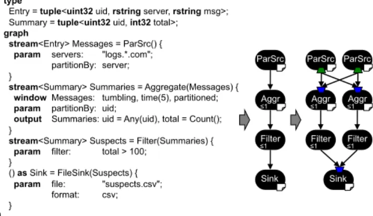
Figure 1: Example SPL program (left), its stream graph (mid-dle), and the parallel transformation of that graph (right). The paper icons in the lower right of an operator indicate that that operator has state, and the numbers in the lower left indicate that operator’s selectivity.
Another way of thinking about selectivity is the consump-tion to producconsump-tion ratio. In synchronous data flow, the ratio is m : n, where m and n can be any integers, but they must be known statically. In our model, the general ratio is 1 :⇤. When an operator fires, it always consumes a single tuple, but it can produce any number of output tuples, including none. This number can be di↵erent at each firing, hence we call this dynamic selectivity.
Figure 1 presents a sample SPL program [13] on the left. The program is a simplified version of a common streaming application: network monitoring. The application continu-ally reads server logs, aggregates the logs based on user IDs, looks for unusual behavior, and writes the results to a file.
The types Entry and Summary describe the structure of the tuples in this application. A tuple is a data item consisting of attributes, where each attribute has a type (such as uint32) and a name (such as uid). The stream graph consists of operator invocations, where operators transform streams of a particular tuple type.
The first operator invocation, ParSrc, is a source, so it does not consume any streams. It produces an output stream called Messages, and all tuples on that stream are of type Entry. The ParSrc operator takes two parameters. The par-titionBy parameter indicates that the data is partitioned on the server attribute that is a part of tuple type Entry. We consider{server} to be the partitioning key for this operator. The Aggregate operator invocation consumes the Messages stream, indicated by being “passed in” to the Aggregate op-erator. The window clause specifies the tuples to operate on, and the output clause describes how to aggregate input tuples (of type Entry) into output tuples (of type Summary). This operator is also partitioned, but this time the key is the uid attribute of the Entry tuples. Because the Aggregate operator is stateful, we consider this operator invocation to have partitioned state. The Aggregate operator maintains separate aggregations for each instance of the partitioning key ({uid} in this case). In general, programmers can pro-vide multiple attributes to partitionBy, and each attribute is used in combination to create the partitioning key. The operator maintains separate state for each partitioning key.2
The Filter operator invocation drops all tuples from the aggregation that have no more than 100 entries. Finally, the FileSink operator invocation writes all of the tuples that represent anomalous behavior to a file.
The middle of Figure 1 shows the stream graph that pro-grammers reason about. In general, SPL programs can spec-ify arbitrary graphs, but the example consists of just a sim-ple pipeline of operators. We consider the stream graph from the SPL source code the sequential semantics, and our work seeks to preserve such semantics. The right of Fig-ure 1 shows the stream graph that our runtime will actually execute. First, the compiler determines that the first three operators have data parallelism, and it allows the runtime to replicate those operators. The operator instances ParSrc and Aggregate are partitioned on di↵erent keys. Because the keys are incompatible, the compiler instructs the runtime to perform a shu✏e between them, so the correct tuples are routed to the correct operator replica. The Filter operator instances are stateless and can accept any tuple. Hence, tuples can flow directly from the Aggregate replicas to the Filter replicas, without another shu✏e. Finally, the FileSink operator instance is not parallelizable, which implies that there must be a merge before it to ensure it sees tuples in the same order as in the sequential semantics.
Note that there are no programmer annotations in the SPL code to enable the extraction of data parallelism. Our compiler inspects the SPL code, performs the allowable trans-formations to the graph, and informs the runtime how to safely execute the application. The operators themselves are written in C++ or Java and have operator models de-scribing their behavior. Our compiler uses these operator models in conjunction with SPL code inspection to extract data parallelism. While this program is entirely declarative, SPL allows programmers to embed custom, imperative logic in operator invocations. Our static analysis includes such custom logic that is expressed in SPL. Many applications do not implement their own operators, and instead only use existing operators. In our example, operators Aggregate, Fil-ter and FileSink come from the SPL Standard Toolkit, and operator ParSrc is user-defined.
Processing element (PE) Unexpanded parallel region Operator instance
Stream
Figure 2: Stream graph, from the compiler’s perspective.
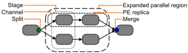
Parts of the stream graph that the compiler determines are safe to parallelize are called parallel regions. To be sys-tem independent, the compiler produces unexpanded parallel regions as shown in Figure 2. Besides auto-parallelization, another important streaming optimization is fusion [10, 15]. Fusion combines multiple operators into a single operating-system process to reduce communication overhead. We refer to fused operators as PE s (processing elements). Our com-piler ensures that PEs never span parallel region boundaries. The runtime expands parallel regions by replicating their PEs as shown in Figure 3. A port is the point where a PE and a stream connect. The runtime implements split as a special form of output port, and merge as a special form
state. Operators obtain keys by hashing the values of the attributes from the partitioning set. So, given a state map, a current tuple and the set of partitioning attributes{a1–an}, each operator firing accesses state[partition(tuple.a1, tuple.a2, ..., tuple.an)].
Stage Channel Split
Expanded parallel region PE replica
Merge
Figure 3: Stream graph, from the runtime’s perspective.
of input port. We refer to each path through an expanded parallel region as a channel. The set of replicas of the same PE is called a stage.
Finally, our runtime is distributed. Each PE can run on a separate host machine, which means that we must carefully consider what information to communicate across PEs.
3. COMPILER
The compiler’s task is to decide which operator instances belong to which parallel regions. Furthermore, the compiler picks implementation strategies for each parallel region, but not the degree of parallelism. One can think of the com-piler as being in charge of safety while avoiding platform-dependent profitability decisions.
3.1 Safety Conditions
This section lists sufficient pre-conditions for auto-parallel-ization. As usual in compiler optimization, our approach is conservative: the conditions may not always be necessary, but they imply safety. The conditions for parallelizing an individual operator instance are:
• No state or partitioned state: The operator instance must be either stateless, or its state must be a map where the key is a set of attributes from the input tuple. Each time the operator instance fires, it only updates its state for the given key. This makes it safe to parallelize by giving each operator replica a disjoint partition of the key domain.
• Selectivity of at most one: As mentioned before, se-lectivity is the number of output tuples per input tuple. Requiring selectivity 1 enables the runtime to imple-ment ordering with a simple sequence number scheme. Note that unlike synchronous data flow [16], SPL sup-ports dynamic selectivity. For example, a filtering oper-ator can have data-dependent predicates where it drops some tuples, but forwards others. Such an operator has a selectivity of 1, as the consumption to production ratio is 1 : [0, 1].
• At most one predecessor and successor: The operator instance must have fan-in and fan-out 1. This means parallel regions have a single entry and exit where the runtime can implement ordering.
The conditions for forming larger parallel regions with mul-tiple operator instances are:
• Compatible keys: If there are multiple stateful operator instances in the region, their keys must be compatible. A key is a set of attributes, and keys are compatible if their intersection is non-empty. Parallel regions are not required to have the exact same partitioning as the oper-ators they contain so long as the region’s partitioning key is formed from attributes that all operators in the region are also partitioned on. In other words, the partitioning
cannot degenerate to the empty key, where there is only a single partition. It is safe to use a coarser partition-ing at the parallel region level because it acts as first-level routing. The operators themselves can still be partitioned on a finer grained key, and that finer grained routing will happen inside the operator itself.
• Forwarded keys: Care must be taken that the region key as seen by a stateful operator instance o indeed has the same value as at the start of the parallel region. This is because the split at the start of the region uses the key to route tuples, whereas o uses the key to access its partitioned state map. All operator instances along the way from the split to o must forward the key unchanged. In other words, they must copy the attributes of the region key unmodified from input tuples to output tuples. • Region-local fusion dependencies: SPL programmers
can influence fusion decisions with pragmas. If the prag-mas require two operator instances to be fused into the same PE, and one of them is in a parallel region, the other one must be in the same parallel region. This ensures that the PE replicas after expansion can be placed on di↵erent hosts of the cluster.
3.2 Compiler Analysis
This section describes how the compiler establishes the safety conditions from the previous section. We must first distinguish an operator definition from an operator invoca-tion. The operator definition is a template, such as an Ag-gregate operator. It provides di↵erent configuration options, such as what window to aggregate over or which function (Count, Avg, etc.) to use. Since users have domain-specific code written in C++ or Java, we support user-defined oper-ators that encapsulate such code. Each operator definition comes with an operator model describing its configuration options to the compiler. The operator invocation is written in SPL and configures a specific instance of the operator, as shown in Figure 1. The operator instance is a vertex in the stream graph.
We take a two-pronged approach to establishing safety conditions: program analysis for operator invocations in SPL, and properties in the operator model for operator definitions. This is a pragmatic approach, and requires some trust: if the author of the operator deceives the compiler by using the wrong properties in the operator model, then our optimiza-tion may be unsafe. This situaoptimiza-tion is analogous to what happens in other multi-lingual systems. For instance, the Java keyword final is a property that makes a field of an ob-ject immutable. However, the author of the Java code may be lying, and actually modify the field through C++ code. The Java compiler cannot detect this. By correctly model-ing standard library operators, and choosmodel-ing safe defaults for new operators that can then be overridden by their authors, we discharge our part of the responsibility for safety.
The following flags in the operator model support auto-parallelization. The default for each is Unknown.
• state 2 {Stateless, ParameterPartitionBy, Unknown}. In the ParameterPartitionBy case, the partitionBy parame-ter in the operator invocation specifies the key.
• selectivity 2 {ExactlyOne, NoParamFilter, AtMostOne, Unknown}. In the NoParamFilter case, the selectivity is = 1 if the op-erator invocation specifies no filter parameter, and 1
otherwise. (In SPL, filter parameters are optional predi-cates which determine if the operator will drop a tuple, or send it downstream.) Using consumption to production ratios, a selectivity of = 1 is 1 : 1, 1 is 1 : [0, 1] and Unknown is 1 : [0,1).
• forwarding 2 {Always, FunctionAny, Unknown}.
In the Always case, all attributes are forwarded unless the operator invocation explicitly changes or drops them. The FunctionAny case is used for aggregate operators, which forward only attributes that use an Any function in the operator invocation.
In most cases, analyzing an SPL operator invocation is straightforward given its operator model. However, oper-ator invocations can also contain imperative code, which may a↵ect safety conditions. State can be a↵ected by mu-tating expressions such as n++ or foo(n), if function foo modifies its parameter or is otherwise stateful. SPL’s type system supports the analysis by making parameter muta-bility and statefulness of functions explicit [13]. Selectivity can be a↵ected if the operator invocation calls submit to send tuples to output streams. Our compiler uses data-flow analysis to count submit-calls. If submit-calls appear inside of if -statements, the analysis computes the minimum and maximum selectivity along each path. If submit-calls appear in loops, the analysis assumes that selectivity is Unknown.
3.3 Parallel Region Formation
After the compiler analyzes all operator instances to de-termine the properties that a↵ect safety, it forms parallel regions. In general, there is an exponential number of pos-sible choices, so we employ a simple heuristic to pick one. This leads to a faster algorithm and more predictable results for users.
Our heuristic is to always form regions left-to-right. In other words, the compiler starts parallel regions as close to sources as possible, and keeps adding operator instances as long as all safety conditions are satisfied. This is motivated by the observation that in practice, more operators are se-lective than prolific, since streaming applications tend to re-duce the data volume early to rere-duce overall cost [26]. Fur-thermore, our policy of only parallelizing operator instances with selectivity 1 ensures that the number of tuples in a region shrinks from left to right. Therefore, our left-to-right heuristic minimizes the number of tuples traveling across region boundaries, where they incur split or merge costs.
o8 o7 n.p. o3 n.p. o4 o12 l o13 o14 o1 o9 k o10 k,l o2 o11 l o5 o6 k
Figure 5: Parallel region formation example. Operator instances labeled “n.p.” are not parallelizable, for example, due to unknown state or selectivity > 1. The letters k and l indicate key attributes. The dotted line from o12 to o14 indicates a fusion dependency. Dashed ovals indicate unexpanded parallel regions as in Figure 2. The paper icons in the lower right of an operator indicate the operator is stateful.
The example stream graph in Figure 5 illustrates our al-gorithm. The first parallel region contains just o1, since its
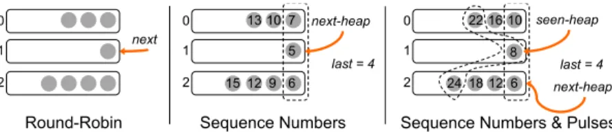
next 0 1 2 next-heap 0 1 2 7 10 13 6 9 12 15 last = 4 next-heap 0 1 2 10 16 22 6 12 18 24 last = 4 5 8 seen-heap
Round-Robin Sequence Numbers Sequence Numbers & Pulses
Figure 4: Merge ordering mechanisms after receiving a new tuple.
next region contains just o2, since its successor o3 is “n.p.”
(not parallelizable). Operator instances o5 and o6 are
com-bined in a single region, since o5is stateless and o6has state
partitioned by key{k}. The region with o9and o10ends
be-fore o11, because adding o11would lead to an empty region
key. This illustrates our left-to-right heuristic: another safe alternative would have been to combine o10with o11instead
of o9. Finally, o12is not in a parallel region, because it has a
fusion dependency with o14. (Recall that programmers can
request that multiple operators be fused together into one PE.) That means they would have to be in the same paral-lel region, but o13is in the way and violates the fan-in = 1
condition.
3.4 Implementation Strategy Selection
Besides deciding which operator instances belong to which parallel region, the compiler also decides the implementation strategy for each parallel region. We refer to the single entry and single exit of a region as the first joint and last joint, respectively. The first joint can be a parallel source, split, or shu✏e. Likewise, the last joint can be a parallel sink, merge, or shu✏e. The compiler decides the joint types, as well as their implementation strategies. Later, the runtime picks up these decisions and enforces them.
Our region formation algorithm keeps track of the region key and overall selectivity as it incrementally adds operator instances to the region. When it is done forming a region, the compiler uses the key to pick a tuple-routing strategy (for example, hashing), and it uses the selectivity to pick an ordering strategy (for example, round-robin). After region formation, the compiler inserts shu✏es between each pair of adjacent parallel regions, and adjusts their joint types and ordering strategies accordingly.
4. RUNTIME
The runtime has two primary tasks: route tuples to par-allel channels, and enforce tuple ordering. Parpar-allel regions should be semantically equivalent to their sequential coun-terparts. In a streaming context, that equivalence is main-tained by ensuring that the same tuples leave parallel re-gions in the same order regardless of the number of parallel channels.
The distributed nature of our runtime—PEs can run on separate hosts—has influenced every design decision. We favored a design which does not add out-of-band commu-nication between PEs. Instead, we either attach the extra information the runtime needs for parallelization to the tu-ples themselves, or add it to the stream.
4.1 Splitters and Mergers
Routing and ordering are achieved through the same mech-anisms: splitters and mergers in the PEs at the edges of par-allel regions (as shown in Figure 3). Splitters exist on the output ports of the last PE before the parallel region. Their
= 1 1 unknown
no state round-robin seqno & pulses n/a partitioned state seqno seqno & pulses n/a
unknown state n/a n/a n/a
Table 1: Ordering strategies determined by state and selectivity. Entries marked n/a are not parallelized.
job is to route tuples to the appropriate parallel channel, and add any information needed to maintain proper tuple ordering. Mergers exist on the input ports of the first PE after the parallel region. Their job is to take all of the dif-ferent streams from each parallel channel and merge those tuples into one, well-ordered output stream. The splitter and merger must perform their jobs invisibly to the opera-tors both inside and outside the parallel region.
4.2 Routing
When parallel regions only have stateless operators, the splitters route tuples in round-robin fashion, regardless of the ordering strategy. When parallel regions have parti-tioned state, the splitter uses all of the attributes that define the partition key to compute a hash value. That hash value is then used to route the tuple, ensuring that the same at-tribute values are always routed to the same operators.
4.3 Ordering
There are three di↵erent ordering strategies: round-robin, sequence numbers, and sequence numbers and pulses. The situations in which the three strategies must be employed depend on the presence of state and the region’s selectivity, as shown in Table 1.
Internally, all kinds of mergers maintain queues for each channel. PEs work on a push, not a pull basis. So a PE will likely receive many tuples from a channel, even though the merger is probably not yet ready to send those tuples downstream. The queues exist so that the merger can accept tuples from the transport layer, and then later pop them o↵ of the queues as dictated by their ordering strategy.
In fact, all of the merging strategies follow the same al-gorithm when they receive a tuple. Upon receiving a tuple from the transport layer, the merge places that tuple into the appropriate queue. It then attempts to drain the queues as much as possible based on the status of the queues and its ordering strategy. All of the tuples in each queue are ordered. If a tuple appears ahead of another tuple in the same channel queue, then we know that it must be submit-ted downstream first. Mergers, then, are actually perform-ing a merge across ordered sources. Several of the orderperform-ing strategies take advantage of this fact.
4.3.1 Round-Robin
The simplest ordering strategy is round-robin, and it can only be employed with parallel regions that have stateless operators with a selectivity of 1. Because there is no state,
the splitter has the freedom to route any tuple to any parallel channel. On the other end, the merger can exploit the fact that there will always be an output tuple for every input tuple. Tuple ordering can be preserved by enforcing that the merger pops tuples from the channel queues in the same order that the splitter sends them.
The left side of Figure 4 shows an example of a round-robin merge. The merger has just received a tuple on chan-nel 1. Chanchan-nel 1 is next in the round-robin order, so the merger will submit the tuple on channel 1. It will also sub-mit the front tuples on 2 and 0, and will once again wait on 1.
4.3.2 Sequence Numbers
The second ordering strategy is sequence numbers, where the splitter adds a sequence number to each outgoing tuple. The PE runtime inside of each parallel channel is responsible for ensuring that sequence numbers are preserved; if a tuple with sequence number x is the cause of an operator sending a tuple, the resulting tuple must also carry x as its sequence number. When tuples have sequence numbers, the merger’s job is to submit tuples downstream in sequential order.
The merger maintains order by keeping track of the quence number of the last tuple it submitted. If that se-quence number is y, then it knows that the next tuple to be submitted must be y + 1; this condition holds because sequence numbers without pulses are used only when the selectivity is 1. The merger also maintains a minimum-heap of the head of each channel queue. The top of the heap is the tuple with the lowest sequence number across all of the channel queues; it is the best candidate to be submit-ted. We call this heap the next-heap. Using a heap ensures that obtaining the next tuple to submit (as required dur-ing a drain) is a log N operation where N is the number of incoming channels.
The middle of Figure 4 shows an example of a sequence number merge which has just received a tuple on channel 1. The merger uses the next-heap to keep track of the lowest sequence number across all channel queues. In this instance, it knows that last = 4, so the next tuple to be submitted must be 5. The top of the next-heap is 5, so it is submitted. Tuples 6 and 7 are also drained from their queues, and the merger is then waiting for 8.
4.3.3 Sequence Numbers and Pulses
The most general strategy is sequence numbers and pulses, which permits operators with selectivity less than 1, mean-ing they may drop tuples. In that case, if the last tuple to be submitted was y, the merger cannot wait until y + 1 shows up—it may never come. But the merger cannot simply use a timeout either, because the channel that y + 1 would come in on may simply be slow. The merger must handle a clas-sic problem in distributed systems: discriminating between something that is gone, and something that is merely slow. Pulses solve this problem. The splitter periodically sends a pulse on all channels, and the length of this period is an epoch. Each pulse receives the same sequence number, and pulses are merged along with tuples. Operators in parallel channels forward pulses regardless of their selectivity; even an operator that drops all tuples will still forward pulses.
The presence of pulses guarantees that the merger will receive information on all incoming channels at least once per epoch. The merger uses pulses and the fact that all
tuples and pulses come in sequential order on a channel to infer when a tuple has been dropped. In addition to the next-heap, the merger maintains an additional minimum-heap of the tuples last seen on each channel, which are the backs of the channel queues. This heap keeps track of the minimum of the maximums; the back of each channel queue is the highest sequence number seen on that channel, and the top of this heap is the minimum of those. We call this heap the seen-heap. Using a heap ensures that finding the min-of-the-maxes is a log N operation.
Consider the arrival of the tuple with sequence number z. As in the sequence number case, if z 1 = last where last is the sequence number of the tuple submitted last, then z is ready to be submitted. If that is not the case, we may still submit z if we have enough information to infer that tuple z 1 has been dropped. The top of the seen-heap can provide that information: if z 1 is less than the top of the seen-heap, then we know for certain that z 1 is never coming. Recall that the top of the seen-heap is the lowest sequence number among the backs of the channel queues (the min-of-the-maxes), and that the channel queues are in sequential order. So we use the seen-heap to check the status of all of the channels. And if z 1 (the tuple that z must wait on) is less than the backs of all of the channel queues, then it is impossible for z 1 to arrive on any channel.
The right of Figure 4 shows an example of a sequence number and pulses merger that has just received a tuple on channel 1. In addition to the next-heap, the merger uses the seen-heap to track the lowest sequence number among the backs of the queues. In this instance, last = 4, so the merger needs to either see 5 or be able to conclude it is never coming. After 8 arrives on channel 1 and becomes the top of the seen-heap, the merger is able to conclude that 5 is never coming—the top of the seen-heap is the lowest sequence number of the backs of the queues, and 5 < 8. The merger then submits 6, and it also has enough information to submit 8. It cannot submit 10 because it does not have enough information to determine if 9 has been dropped.
4.4 Shuffles
When the compiler forms parallel regions (Section 3.3), it aggressively tries to merge adjacent regions. Adjacent parallel regions that are not merged are sequential bottle-necks. When possible, the compiler merges parallel regions by simply removing adjacent mergers and splitters. Sec-tion 3.1 lists the safety condiSec-tions for when merging parallel regions is possible. However, when adjacent parallel regions have incompatible keys, they cannot be merged. Instead, the compiler inserts a shu✏e: all channels of the left par-allel region end with a split, and all channels of the right parallel region begin with a merge. Shu✏es preserve safety while avoiding a sequential bottleneck.
In principle, shu✏es are just splits and merges at the edges of adjacent parallel regions. However, splits and merges in a shu✏e modify their default behavior, as shown in Figure 7. Ordinary splitters have both routing and ordering respon-sibilities. The ordering responsibility for an ordinary splitter is to create and attach sequence numbers (if needed) to each outgoing tuple. When tuples arrive at a splitter in a shu✏e, those tuples already have sequence numbers. The PE itself preserves sequence numbers, so a splitter in a shu✏e only has routing responsibilities. Splitters inside of a shu✏e also
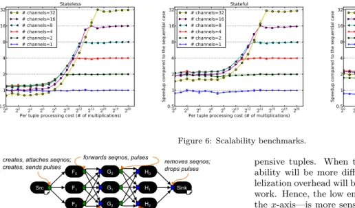
Figure 6: Scalability benchmarks. H1 F0 Src F1 F2 H0 H2 Sink
creates, attaches seqnos; creates, sends pulses
forwards seqnos, pulses
G1
G0
G2
removes seqnos; drops pulses
forwards seqnos; receives N pulses, forwards 1
Figure 7: Splitter and merger responsibilities in a shu✏e.
do not generate pulses; they were already generated by the splitter at the beginning of the parallel region.
When mergers exist at the edge of parallel regions, they are responsible for stripping o↵ the sequence numbers from tuples and dropping pulses. Mergers that are a part of a shu✏e must preserve sequence numbers and pulses. But they cannot do so naively, since mergers inside of a shu✏e will actually receive N copies of every pulse, where N is the number of parallel channels. The split before them has to forward each pulse it receives to all of the mergers in the shu✏e, meaning that each merger will receive a copy of each pulse. The merger prevents this problem from exploding by ensuring that only one copy of each pulse is fowarded on through the channel. If the merger did not drop duplicated pulses, then the number of pulses that arrived at the final merger would be on the order of Ns where s is the number
of stages connected by shu✏es.
5. RESULTS
We use three classes of benchmarks. The scalability bench-marks are designed to show that simple graphs with data parallelism will scale using our techniques. Our microbench-marks are designed to measure the overhead of runtime mechanisms that are necessary to ensure correct ordering. Finally, we use five application kernels to show that our techniques can improve the performance of stream graphs inspired by real applications.
All of our experiments were performed on machines with 2 Intel Xeon processors where each processor has 4 cores. In total, each machine has 8 cores and 64 GB of memory.
Our Large-scale experiment uses 112 cores across 14 ma-chines. The large-scale experiments demonstrate the inher-ent scalability of our runtime, and indicate that the linear trends seen in the other experiments are likely to continue. The remainder of our experiments use 4 machines connected with Infiniband.
We vary the amount of work per tuple on the x-axis, where work is the number of integer multiplications performed per tuple. We scale this exponentially so that we can explore how our system behaves with both very cheap and very
ex-pensive tuples. When there is little work per tuple, scal-ability will be more difficult to achieve because the paral-lelization overhead will be significant compared to the actual work. Hence, the low end of the spectrum—the left side of the x-axis—is more sensitive to the runtime parallelization overheads. The high end of the spectrum—the right side of the x-axis—shows the scalability that is possible when there is sufficient work.
All data points in our experiments represent the average of at least three runs, with error bars showing the standard deviation.
5.1 Scalability Benchmarks
The scalability benchmarks, Figure 6, demonstrate our runtime’s scalability across a wider range of parallel chan-nels. These experiments use 4 machines (32 cores). When there is a small amount of work per tuple (left side of the x-axis), these experiments also show how sensitive the runtime is to having more active parallel channels than exploitable parallelism.
The Stateless scalability experiment has a stream graph with a single stateless operator inside of a parallel region. Because the operator in the parallel region is stateless, the compiler recognizes that the runtime can use the least ex-pensive ordering strategy, round-robin. Hence, we observe linear scalability, up to 32 times the sequential case when 32 parallel channels are used with 32 cores available. Just as importantly, when there is very little work—when the amount of work to be done is closer to the parallelization cost—additional parallel channels do not harm performance. The stream graph is the same for the Stateful scalabil-ity experiment, but the operator is an aggregator that has local state. The compiler instructs the runtime to use se-quence numbers and pulses to ensure proper ordering. The scalability is linear for 2–16 parallel channels, and achieves 31.3 times the sequential case for 32 parallel channels when using 32 cores. However, all cases see some performance improvement with very inexpensive work, with all but the 32-channel cases never dropping below 2 times improvement. The 32-channel case never has less than 1.4 time improve-ment for very inexpensive work. This result indicates that our runtime has little overhead. Note that in the Stateful experiment, inexpensive work exhibits more than 2 times improvement for 1–8 channels, which is not the case with the Stateless experiment. Even though the per-tuple cost is the same for both experiments, the aggregation itself adds a fixed cost. Hence, operators in the Stateful experiment do more work than operators in the Stateless experiment.
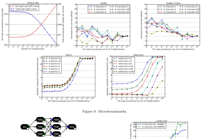
Figure 8: Microbenchmarks. Aggr Aggr Src Aggr Aggr Aggr Aggr Sink ≤1 ≤1 ≤1 ≤1 ≤1 ≤1
Figure 9: Expanded stream graph for a two-way shu✏e.
Very inexpensive work in the Stateful experiment is benefit-ing from both pipeline and data parallelism.
Figure 9 shows the stream graph for the Shu✏e experi-ment, which has two aggregations partitioned on di↵erent keys, requiring a shu✏e between them. When there are 32 channels in the Shu✏e experiment, there are actually 64 processes running on 32 cores. Hence, the 32-channel case is an over-subscribed system by a factor of 2, and it only scales to 22.6 times. The 16-channel case has 32 PEs, which is a fully subscribed system, and it scales to 15.3 times. As with the Stateful experiment, the inexpensive end of the work spectrum benefits from pipeline as well as data parallelism, achieving over 2 times improvement for 4–32 channels.
Note that the e↵ect of pipeline parallelism for low tuple costs is least pronounced in the Stateless experiment, and most pronounced in Shu✏e. In the sequential case with low-tuple costs, the one PE worker is the bottleneck; it must receive, process, and send tuples. The splitter only sends tuples. As the number of parallel channels increases, the work on each worker PE decreases, making the splitter the bottleneck. The more costly the work is, the stronger the e↵ect becomes, which is why it is weakest in the Stateless experiment and strongest in the Shu✏e experiment.
The Large-scale experiment in Figure 10 demonstrates the scalability the runtime system is able to achieve with a large number of cores across many machines. This experiment uses a total of 14 machines. One machine (8 cores) is ded-icated to the source and sink, which includes the split and merge at the edges of the parallel region. The other 13 machines (104 cores) are dedicated to the PEs in the
par-
Figure 10: Large-scale scalability.
allel region. The stream graph for the stateful experiment is a single, stateful aggregation in a parallel region with 100 parallel channels. The stateful experiment shows near linear scalability, maxing out at 93 times improvement.
The shu✏e experiment in Figure 10 has the same stream graph as shown in Figure 9. As explained with the Shu✏e experiment, there are twice as many processes as parallel channels. When there are 50 parallel channels in each of its two parallel regions, it maxes out at 42 times improvement. The shu✏e experiment cannot scale as high as the stateful experiment because with 50 parallel channels, there are 100 PEs.
5.2 Microbenchmarks
All of the microbenchmarks are shown in Figure 8. The stream graph for all of the microbenchmarks is a parallel region with a single stateless operator.
The Time & Rate benchmark shows the relationship be-tween the amount of work done and the time it takes to do that work. For all our of results, we characterize the work done in the number of multiplications performed per tuple. This experiment maps those multiplications to both an elapsed time (left y-axis) and a processing rate (right
y-axis). The elapsed time range is from 600 nanoseconds to 1 millisecond, and the processing rate is from 1.6 mil-lion tuples a second to one thousand tuples a second. This cost experiment is a “calibration” experiment that shows the relationship between the amount of work done, the time it takes to do that work, and the throughput on all of our other experiments.
As described in Section 4.3, adding sequence numbers to tuples and inserting pulses on all channels will incur some overhead. We measured this overhead in Figure 8, using pure round-robin ordering as the baseline. As expected, as the work-per-tuple increases, the cost of adding a sequence number to each tuple becomes negligible compared to the actual work done. However, even when relatively little work is done, the highest average overhead is only 12%. Pulses add more overhead, but never more than 21%. As with sequence numbers alone, the overhead goes towards zero as the cost of the work increases.
Epochs, as explained in Section 4.3, are the number of tu-ples on each channel between generating pulses on all chan-nels. The Epoch experiment in Figure 8 measures how sen-sitive performance is to the epoch length. An epoch of e means that the splitter will send eN tuples, where N is the total number of channels, before generating a pulse on each channel. We scale the epoch with the number of channels to ensure that each channel receives e tuples before it receives a single pulse. The default epoch is e = 10. Our results show that beyond an epoch length of 8, speedup does not vary more than 8% in the range 8–32.
In the Selectivity experiment, we fixed the number of par-allel channels at 32. Each line in the graph represents a progressively more selective aggregator. So, when selectiv-ity is 1:1, the operator performs an aggregation for every tuple it receives. When selectivity is 1:256, it performs 1 aggregation for every 256 tuples it receives. When per-tuple cost is low, and the selectivity increases, the worker PEs do very little actual work; they mostly receive tuples. However, the cost for the splitter remains constant, as it always has 32 channels. When selectivity is high, the splitter is paying the cost to split to 32 channels, but there is no benefit to doing so, since real work is actually a rare event. As a result, as selectivity increases, there is actually slowdown until the cost of processing one of the selected tuples become large.
5.3 Application Kernels
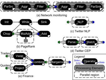
This section further explores performance using five real-world application kernels shown in Figure 11. All of these application kernels have selective or stateful parallel regions, which require the techniques presented in this paper to be parallelized. They are representative of big data use cases.
The Network monitoring kernel monitors multiple servers, looking for suspicious user behavior. The filters remove val-ues below a “suspicious” threshold. The left parallel region is partitioned by the server, while the right parallel region is partitioned by users, with a shu✏e in the middle. Note, however, that because there are parallel sources on the left and parallel sinks on the right, tuples are not ordered in this application. The compiler recognizes this and informs the runtime that it has only routing responsibilities.
The PageRank kernel uses a feedback loop to iteratively rank pages in a web graph [18]. This application is typically associated with MapReduce, but is also easy to express in a streaming language. Each iteration multiplies the rank
Parse Match Vwap Project Combine Bargains Trades Quotes MulAdd Add Chop While Sink Init
ParSrc Aggr Filter Aggr Filter ParSink
NLP
(a) Network monitoring
(b) PageRank (c) Twitter NLP (d) Twitter CEP (e) Finance Operator Processing Element Parallel region Legend: ≤1 ≤1 ≤1 ≤1 ≤1 ≤1 ≤1 ≤1 Selec- tivity State
Figure 11: Stream graphs for the application kernels. operators
Network Left 33 µs Right 23 µs
PageRank MulAdd 11 s
Twitter NLP NLP 103 µs
Twitter CEP Parse 140 µs Match 3.5 ms
Finance Vwap 81 µs Project 26 µs Bargains 2.5 µs Table 2: Average processing time per tuple.
vector with the web graph adjacency matrix. In the first iteration, MulAdd reads the graph from disk. Each iteration uses the parallel channels of MulAdd to multiply the previous rank vector with some rows of the matrix, and uses Add to assemble the next rank vector. The input consists of a synthetic graph of 2 million vertices with a sparsity of 0.001, in other words, 4 billion uniformly distributed edges.
The Twitter NLP kernel uses a natural language process-ing engine [5] to analyze tweets. The input is a stream of tweet contents as strings, and the output is a tuple contain-ing a list of the words used in the message, a list with the lengths of the words, and the average length of the words. The stream graph has a parallel region with a single, state-less, operator. The NLP engine is implemented in Java, so tuples that enter the NLP operator must be serialized, copied into the JVM, processed, then deserialized and copied out from the JVM.
The Twitter CEP kernel uses complex event processing to detect patterns across sequences of tweets [12]. The Parse operator turns an XML tweet into a tuple with author, contents, and timestamp. The Match operator detects se-quences of five consecutive tweets by the same author with identical hash-tags. This pattern is a pathological case for this input stream, which causes the finite state machine that implements the pattern matching to generate and check many partial matches for most tuples. Both Parse and Match are parallelized, with a shu✏e to partition by author before Match. The topology is similar to that of the Network mon-itoring kernel, but since there is no parallel source or sink, ordering matters.
The Finance kernel detects bargains when a quote exceeds the VWAP (volume-weighted average price) of its stock sym-bol. The graph has three parallelizable operators. Only the Combine operator, which merges its two input streams in timestamp order, is not parallel.
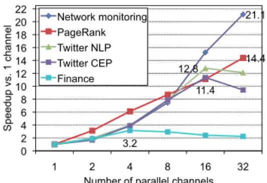
applica-21.1 14.4 12.8 11.4 3.2 0 2 4 6 8 10 12 14 16 18 20 22 1 2 4 8 16 32 Speedup vs. 1 channel
Number of parallel channels Network monitoring
PageRank Twitter NLP Twitter CEP Finance
Figure 12: Performance results for the application kernels.
tion kernels on a cluster of 4 machines with 8 cores each, for a total of 32 cores. In these experiments, all parallel regions are replicated to the same number of parallel channels. For example, when the number of channels is 32, Twitter CEP has a total of 64 operator instances, thus over-subscribing the cores. Most of the kernels have near-perfect scaling up to 8 channels. The exception is Finance, which tops out at a speedup of 3.2⇥ with 4 channels, at which point the Com-bine operator becomes the bottleneck. The other application kernels scale well, topping out at either 16 or 32 channels, with speedups between 11.4⇥ and 21.1⇥ over sequential.
Table 2 shows the average time it takes for all operators in parallel regions to process tuples. Combining this data with the Time & Rate experiment in Figure 8 allows us to cali-brate the application kernels to the scalability benchmarks in Figure 6. Note, however, that this is a rough calibration, as the integer multiplications in the microbenchmarks occur in a tight loop, operating on a register. The average timings in Table 2 will include a mix of integer and floating point operations that could potentially include cache misses and branch mispredictions.
6. RELATED WORK
Table 3 compares this paper to prior work on data-parallel streaming. Stateful indicates whether the parallelizer can handle stateful operators, which are necessary for aggre-gation, enrichment, and detecting composite events across sequences of tuples. Dynamic indicates whether the paral-lelizer can handle operators with dynamic selectivity, which are necessary for data-dependent filtering, compression, and time-based windows. Safety indicates whether the paral-lelizer guarantees that the order of tuples in the output stream is the same as without parallelization, which is nec-essary for deterministic applications and simplifies testing and accountability. Finally, Scaling indicates the maximum number of cores for which results were reported. Our work is the first that is both general (with respect to state and dy-namism) and safe. Furthermore, our paper includes results for scaling further than prior stream-processing papers.
The compiler for the StreamIt language auto-parallelizes operators using round-robin to guarantee ordering [10]. The StreamIt language supports stateful and dynamic operators, but the StreamIt auto-parallelization technique only works for operators that are stateless and have static selectivity. We treat it as a special case of our more general framework, which also supports stateful operators and dynamic selec-tivity. Furthermore, unlike StreamIt, we support more
gen-Auto-parallel Generality Safety Scaling
streaming system Stateful Dynamic Order #Cores
StreamIt [10] no no yes 64
PS-DSWP [21] no no yes 6
Brito et al. [3] yes no yes 8
Elastic operators [22] no yes no 16
S4 [17] yes yes no 64
This paper yes yes yes 100
Table 3: Comparison to prior work on parallel streaming.
eral topologies that eliminate bottle-necks, including parallel sources, shu✏es, and parallel sinks.
To achieve our scaling results for stateful operators, we adapt an idea from distributed databases [9, 11]: we parti-tion the state by keys. This same technique is also the main factor in the success of the MapReduce [8] and Dryad [14] batch processing systems. However, unlike parallel databases, MapReduce, and Dryad, our approach works in a streaming context. This required us to invent novel techniques for en-forcing output ordering. For instance, MapReduce uses a batch sorting stage for output ordering, but that is not an option in a streaming system. Furthermore, whereas parallel databases rely on relational algebra to guarantee that data parallelism is safe, MapReduce and Dryad leave this up to the programmer. Our system, on the other hand, uses static analysis to infer sufficient safety preconditions.
There are several e↵orts, including Hive [25], Pig [20] and FlumeJava [4], that provide higher-level abstractions for MapReduce. These projects provide a programming model that abstracts away the details of using a high performance, distributed system. Since these languages and libraries are abstractions for MapReduce, they do not work in a stream-ing context, and do not have the orderstream-ing guarantees that our system does.
There has been prior work on making batch data process-ing systems more incremental. MapReduce Online reports approximate results early, and increases accuracy later [7]. The Percolator allows observers to trigger when intermediate results are ready [19]. Unlike these hybrid systems, which still experience high latencies, our system is fully streaming. Storm is an open-source project for distributed stream computing [24]. The programming model is similar to ours— programmers implement asynchronous bolts which can have dynamic selectivity. Developers can achieve data parallelism on any bolt by requesting multiple copies of it. However, such data parallelism does not enforce sequential semantics; safety is left entirely to the developers. S4 is another open-source streaming system [17], which was inspired by both MapReduce and the foundational work behind System S [1]. In S4, the runtime creates replica PEs at runtime for each new instance of a key value. Creating replica PEs enables data parallelism, but S4 has no mechanisms to enforce tuple ordering. Again, safety is left to developers.
There are extensions to the prior work on data-flow par-allelization that are complementary to our work. River per-forms load-balancing for parallel flows [2], and Flux supports fault-tolerance for parallel flows [23]. Both River and Flux focus on batch systems, and both leave safety to the user. Elastic operators [22] and flexible filters [6] adapt the de-gree of parallelism dynamically, but do not address stateful operators in a distributed system or safey analysis. Finally, Brito et al. describes how to parallelize stateful operators with STM (software transactional memory) [3], but only if memory is shared and operator selectivity is exactly one.
7. CONCLUSIONS
We have presented a compiler and runtime system that are capable of automatically extracting data parallelism from streaming applications. Our work di↵ers from prior work by being able to extract such parallelism with safety guar-antees in the presence of operators that can be stateful, se-lective, and user-defined. We have demonstrated that these techniques can scale with available resources and exploitable parallelism. The result is a programming model in which de-velopers can naturally express task and pipeline parallelism, and let the compiler and runtime automatically exploit data parallelism.
Acknowledgements
We would like to thank Rohit Khandekar for modifying the fusion algorithm implementation to accommodate the changes in the stream graph caused by auto-parallelization. We would also like to thank the anonymous reviewers whose detailed feedback substantially improved our paper.
8. REFERENCES
[1] L. Amini, H. Andrade, R. Bhagwan, F. Eskesen, R. King, P. Selo, Y. Park, and C. Venkatramani. SPC: A distributed, scalable platform for data mining. In International Workshop on Data Mining Standards, Services, and Platforms, 2006.
[2] R. H. Arpaci-Dusseau, E. Anderson, N. Treuhaft, D. E. Culler, J. M. Hellerstein, D. Patterson, and K. Yelick. Cluster I/O with River: Making the fast case common. In Workshop on I/O in Parallel and Distributed Systems (IOPADS), 1999.
[3] A. Brito, C. Fetzer, H. Sturzrehm, and P. Felber. Speculative out-of-order event processing with software transaction memory. In Conference on Distributed Event-Based Systems (DEBS), 2008. [4] C. Chambers, A. Raniwala, F. Perry, S. Adams, R. R.
Henry, R. Bradshaw, and N. Weizenbaum. FlumeJava: easy, efficient data-parallel pipelines. In Proceedings of the 2010 ACM SIGPLAN conference on Programming Language Design and Implementation (PLDI), 2010. [5] L. Chiticariu, R. Krishnamurthy, Y. Li, S. Raghavan,
F. R. Reiss, and S. Vaithyanathan. SystemT: an algebraic approach to declarative information
extraction. In Proceedings of the 48th Annual Meeting of the Association for Computational Linguistics (ACL), 2010.
[6] R. L. Collins and L. P. Carloni. Flexible filters: Load balancing through backpressure for stream programs. In International Conference on Embedded Software (EMSOFT), 2009.
[7] T. Condie, N. Conway, P. Alvaro, J. M. Hellerstein, K. Elmeleegy, and R. Sears. MapReduce online. In Networked Systems Design and Implementation, 2010. [8] J. Dean and S. Ghemawat. MapReduce: Simplified
Data Processing on Large Clusters. In Operating Systems Design and Implementation (OSDI), 2004. [9] D. J. Dewitt, S. Ghandeharizadeh, D. A. Schneider,
A. Bricker, H. I. Hsiao, and R. Rasmussen. The Gamma database machine project. Transactions on Knowledge and Data Engineering, 2(1), 1990.
[10] M. I. Gordon, W. Thies, and S. Amarasinghe. Exploiting coarse-grained task, data, and pipeline parallelism in stream programs. In Architectural Support for Programming Languages and Operating Systems (ASPLOS), 2006.
[11] G. Graefe. Encapsulation of parallelism in the Volcano query processing system. In International Conference on Management of Data (SIGMOD), 1990.
[12] M. Hirzel. Partition and compose: Parallel complex event processing. In Conference on Distributed Event-Based Systems (DEBS), 2012.
[13] M. Hirzel, H. Andrade, B. Gedik, V. Kumar, G. Losa, M. Mendell, H. Nasgaard, R. Soul´e, and K.-L. Wu. Streams processing language specification. Research Report RC24897, IBM, 2009.
[14] M. Isard, M. B. Y. Yu, A. Birrell, and D. Fetterly. Dryad: Distributed data-parallel program from sequential building blocks. In European Conference on Computer Systems (EuroSys), 2007.
[15] R. Khandekar, I. Hildrum, S. Parekh, D. Rajan, J. Wolf, K.-L. Wu, H. Andrade, and B. Gedik. COLA: Optimizing stream processing applications via graph partitioning. In International Conference on
Middleware, 2009.
[16] E. A. Lee and D. G. Messerschmitt. Synchronous data flow. Proceedings of the IEEE, 75(9), 1987.
[17] L. Neumeyer, B. Robbins, A. Nair, and A. Kesari. S4: Distributed stream processing platform. In KDCloud, 2010.
[18] L. Page, S. Brin, R. Motwani, and T. Winograd. The pagerank citation ranking: Bringing order to the web. Technical Report 1999-66, Stanford InfoLab,
November 1999.
[19] D. Peng and F. Dabek. Large-scale incremental processing using distributed transactions and notifications. In Operating Systems Design and Implementation (OSDI), 2010.
[20] Pig. http://pig.apache.org/. Retrieved July, 2012. [21] E. Raman, G. Ottoni, A. Raman, M. J. Bridges, and
D. I. August. Parallel-stage decoupled software pipelining. In Code Generation and Optimization (CGO), 2008.
[22] S. Schneider, H. Andrade, B. Gedik, A. Biem, and K.-L. Wu. Elastic scaling of data parallel operators in stream processing. In International Parallel & Distributed Processing Symposium (IPDPS), 2009. [23] M. A. Shah, J. M. Hellerstein, and E. Brewer. Highly
Available, Fault-Tolerant, Parallel Dataflows. In International Conference on Management of Data (SIGMOD), 2004.
[24] Storm. http://storm-project.net/. Retrieved July, 2012.
[25] A. Thusoo, J. S. Sarma, N. Jain, Z. Shao, P. Chakka, S. Anthony, H. Liu, P. Wycko↵, and R. Murthy. Hive: a warehousing solution over a map-reduce framework. Proc. VLDB Endow., 2(2):1626–1629, Aug. 2009. [26] D. Turaga, H. Andrade, B. Gedik, C. Venkatramani,
O. Verscheure, J. D. Harris, J. Cox, W. Szewczyk, and P. Jones. Design principles for developing stream processing applications. Software—Practice and Experience (SP&E), 40(12), Nov. 2010.