'^‘ .c ' ,c:^f ¿-’'",..
.n¿
i^ ^ ïrpJT E O f 'Ξι;c.> '”"· »*”·■· ‘’ ‘w . ',· .' */ ^ , 4
A DISSERTATION SUBMITTED TO
THE DEPARTMENT OF COMPUTER ENGINEERING AND INFORMATION SCIENCE
AND THE INSTITUTE OF ENGINEERING AND SCIENCE OF BILKENT UNIVERSITY
IN PARTIAL FULFILLMENT OF THE REQUIREMENTS FOR THE DEGREE OF
DOCTOR OF PHILOSOPHY
i>y
Talisiii Mertefe Kur(,· .
June 1997
degree of doctor of philosophy.
Assoc. Prof. Ce\raet Aykanat (Supervisor)
I certify that I have read this thesis and that in rny opinion it is fully adequate, in scope and in quality, as a dissertation for the degree of doctor of philosophy.
Prof. Bülent Özgüç (Co-supervisor)
I certify that I have read this thesis and that in my opinion it is fully adequate, in scope and in quality, as a dissertation for the degree of doctor of philosophy.
degree of doctor of philosophy.
I certify that I have read this thesis and that in my opinion it is fully adequate, in scope and in quality, as a dissertation for the degree of doctor of philosophy.
sst. Pro
r
Asst. Prof. Özgür Uluso)
Approved by the Institute of Engineering and Science:
Prof. Mehmet Bat
PARALLEL RENDERING ALGORITHMS FOR
DISTRIBUTED-xMEMORY MULTICOMPUTERS
Tahsin Mertefe Kurç
Ph.D. in Computer Engineering and Information Science
Supervisors:
Assoc. Prof. Cevdet Aykamıt and Prof. Bülent Özgüç
June 1997
In this thesis, utilization of distributed memory multicomputers in gathering radios- ity, polygon rendering and volume rendering is investigated.
In parallel gathering racliosity, the target issues are the parallelization of the com putation of the form-factor matrix and solution phases on hypercube-connected multi- computers. Interprocessor communication in matrix computation phase is decreased by sharing the memory space between matrix elements and the scene data. A demand- driven algorithm is proposed for l)etter computational load balance during calculation of form-factors. Gauss-.Jacobi (G J ) iterative algorithm is used by all of the previous works in the solution phase. We apply more efficient Scaled Conjugate-Gradient (S C G ) algorithm in the solution phase. Parallel algorithms were developed for G J and S C G algorithms for hypercube-connected multicomputers. In addition, load balancing in the tion pha.se is investigated. An efficient data redistribution scheme is proposed, kliis
Object-space parallelism is investigated for parallel polygon rendering on hypercube- connected multicomputers. Briefly, in object-space parallelism, scene data is partitioned into disjoint sets among processors. Each processor performs the rendering of its local partition of primitives. After this local rendering phase, full screen partial images in each processor are merged to obtain the final image. This phase is called pixel merging phase. Pixel merging phase requires interprocessor communication to merge partial images. In this work, hypercube interconnection topology and message passing structure are exploited to merge partial images efficiently. Volume o f communication in pixel merging phase is decreased by only exchanging local foremost pixels in each processor after local rendering phase. For this purpose, a modified scanline z-buffer algorithm is proposed for the local rendering phase. This algorithm avoids message fragmentation by storing local foremost pixels in consecutive memory locations. In addition, it eliminates initialization of z-buffer, which is a sequential overhead to parallel e.xecution. For pixel merging phase, we propose two schemes referred to here as pairwise exchange scheme and all-to- all personalized communication scheme, which are suited to the hypercube topology. We investigate load balancing in pixel merging phase. Two heuristics, recursive subdivision and heuristic bin packing, were proposed to achieve better load balancing in pixel merging phase. These heuristics are adaptive such that they utilize the distribution of foremost pixels on the screen to subdivide the screen in the pixel merging phase.
Image-space parallelism is investigated for parallel volume rendering of unstructured grids. In image-space parallelism, the screen is subdivided into regions. Each processor is assigned one or more subregions. The primitives (e.g.. tetrahedrals) in the volume data are distributed among processors according to screen subdivision and processor-subregion assignments. Then, each processor renders its local subregions. The target topic in this work is the adaptive subdivision of the screen. Adaptive subdivision issue has not been investigated in parallel volume rendering of unstructured grids before. Only some re searchers utilized adaptive subdivision in parallel polygon rendering and ray tracing. In this work, several algorithms are proposed to subdivide the screen adaptively. The algorithms presented in this work can be grouped into two classes: 1-dimensional array
subdivision algorithms are new approaches in parallel rendering field. An experimental comparison of the subdivision algorithms are performed on a common frame work. The subdivision algorithms were employed in the parallelization of a volume rendering algo rithm, which is a polygon rendering based algorithm. In the previous works on parallel polygon rendering, only the number of primitives in a subregion were used to approxi mate the work load of the subregion. We experimentally show that this approximation is not enough. Better speedup values can be obtained by utilizing other criteria such as number of pixels, number of spans in a region. By utilizing these additional criteria, the speedup values are almost doubled.
ÇOK İ
ş l e m c i l i d a g i t i k-
h a f i z a l i bİ
l gİ
s a y a r l a r d aPARALEL G Ö RÜ N TÜ LEM E A L G O R İT M A L A R I
Tahsin Mertefe Kıırç
Bilgisayar ve Enformatik Mühendisliği Doktora
Tez Yöneticileri:
Doç. Dr. Cevdet Ay kanat and Prof. Bülent Özgüç
Haziran 1997
Bu tezde dağıtık hafızalı çok işlemcili bilgisayarların ı.ftma yönteminin toplama meto dunda, poligon görüntülemede ve hacim görüntülemede kullanımı araştırılmıştır.
Toplama metodunda ele alman temel konular durum-katsayı matrisinin hesaplanması ve çözüm adımının hiperküp bağlantılı çoklu bilgisayarlarda paralel olarak yapılmasıdır. Durum-katsayı matrisinin hesaplanmasında işlemciler arası veri aktarımı her işlemcideki hafızanın durum-katsayı matrisi ve ışıma metoduyla görüntülenen ortamı oluşturan ver iler arasında paylaştırılması ile azaltılmıştır. İşlemcilerin daha verimli kullanılabilmesi için dinamik paylaştırma yöntemi uygulanmıştır. Ç'özüın aşamasında Scaled Conjugate- Gradient metodu başarılı bir şekilde uygulanmıştır. Gauss-.iacobi ve Scaled (.'onjugate- Gradient metodları için verimli paralel algoritmalar geliştirilmiştir. Durum-katsayı ma trisinin hesaplanınasnıdan sonra, her işlemcide kalan sıfırdan farklı durum-katsayı de ğerlerinin işlemciler arasında tekrar dağıtılması ile hemen hemen ideal yük dağılımı sağlanmıştır.
işlemciler arasında dağıtılır. Her işlemci kendi parçalarının üzerinde görüntüleme algo ritmalarını çalıştırır. Daha sonra her işlemcideki resimler birleştirilerek son resim ortaya çıkarılır. Bu çalışmada hiperküp bilgisayarında parça uzayında paralelleştirme algo ritmaları geliştirilmiştir. Resimlerin birleştirilmesi sıra.sında işlemciler arasında iletişim hacmini azaltan verimli algoritmalar önerilmiştir, işlemciler arasındaki mesajların kopuk kopuk olmasını önlemek için değiştirilmiş bir görüntüleme algoritması önerilmiştir.
Hacim görüntülemede ise ekran uzayında paralelleştirme yaklaşımı araştırılmıştır. Bu yaklaşımda ekran uzayı işlemciler arasında bölünür. Her işlemci kendisine ait olan ekran parçası üzerinde görüntüleme algoritmasını çalıştırtır. Ekranın bölünmesine göre hacim elernanlarıda işlemciler arasında dağıtılır. Bu çalışmada, çeşitli ekran uzayında bölme yöntemleri incelendi ve geliştirildi. Bu yöntemler ekranı hacim elemanlarının ekrandaki dağılımlarına göre bölerek daha iyi yük dağılımı sağlar. Bu yöntemlerden çizge parçalamaya dayalı bölme ve Hilbert eğrisine dayalı bölme yeni yöntemlerdir. Bu yöntemler deneysel olarak karşılaştırılmıştır. Ayrıca, bu çalışmada incelenen ve geliştirilen yöntemler poligon görüntülemeye dayalı bir hacim görüntüleme algoritmasına başarı ile uygulanmışladır.
I wish to express my deepest gratitude and thanks to Assoc. Prof. Dr. Cevdet Aykanat and Prof. Dr. Bülent Özgüç for their supervision, encouragement, and invalu able advice throughout the development of this thesis.
I am very grateful to Prof. Dr. Semih Bilgen, Asst. Prof. Dr. Özgür Ulusoy, and •Asst. Prof. Dr. Mustafa Pınar for carefully reading my thesis, for their remarks and suggestions.
I would like to extend my sincere thanks to all of my friends for their morale support and encouragement during the thesis work. I would like to thank Egemen Tanin for his sequential volume rendering code. I owe special thanks to all members of our department for providing a pleasant environment for study.
Finally, my sincere thanks goes to my family for their endless morale support and patience.
This work was partially supported by the Scientific and Technical Research Council o f Turkey (TÜ BİTAK ) under grants EEEAG-5 and EEEAG-160, Intel Supercomputer Systems Division under grant SSD100791-2, and the Commission o f the European Com
1 Introduction 1
1.1 Gathering Radiosity .3
1.2 Polygon R e n d e r in g ... 5
1.3 Volume Rendering ... .5
1.4 Contributions of the Thesis ... 7
1.4.1 Parallel Gathering R adiosity... 8
1.4.2 Parallel Polygon Rendering 9 1.4.3 Parallel Volume R endering... 10
1.5 Organization of the T h e s is ... 11
2 Gathering Radiosity on Hypercubes 13 2.1 Gathering Radiosity ... 15
2.1.1 Form-Factor Computation P h a s e ... 16
2.1.2 Solution Phase ... 17
2.2 Previous Work on Parallel Gathering Radiosity 23 2.3 Intel’s iPSC/2 Hypercube Multicomputer... 24
2.4 Parallel Computation of the Form-Factor M a trix ... 27
2.4.1 Static Assignment ... 27
2.4.2 Demand-Driven Assignment Scheme 31 2.5 Parallel Solution P h a s e ... 32
2.5.1 Parallel Gauss-Jacobi M e t h o d ... 32
2.5.2 Parallel Scaled Conjugate-Gradient Method 35 2.5.3 A Parallel Renumbering Scheme... 37
2.6 Load Balancing in the Solution Phase: Data Redistribution... 39
2.6.1 A Parallel Data Redistribution S c h e m e ... 40
2.6.2 Avoiding the Extra Setup Time Overhead 42 2.7 Experimental R e s u lts ... 42
2.8 C on clu sion s... 47
Polygon Rendering: Overview and Related Work 50 3.1 Sequential Polygon R e n d e rin g ... 50
3.1.1 Reading Environment D escription... .50
3.1.2 Lighting C alculations... 52
3.1.3 Geometry P rocessin g ... .52
3.1.4 Shading and Hidden-surface R e m o v a l... .53
3.2 Previous Works on Parallel Polygon R endering... 57
3.2.1 .A Taxonomy of Parallelism in Polygon Rendering on Distributed-Memory M ulticom puters... 57
3.2.2 Previous Works on Parallel Polygon Rendering... 62
3.3 Discussion of Previous Works 71 Active Pixel Merging on Hypercubes 74 4.1 Some Definitions ... 75
4.2 The Parallel A lg o rith m ... 75
4.3 A Modified Scanline Z-buffer Algorithm ... 76
4.4 Pixel Merging on Hypercube M u lticom p u ter... 78
4.4.1 Ring Exchange S ch em e... 78
4.4.2 2-dimensional Mesh Exchange S c h e m e ... 80
4.4.3 K-dimensional Mesh Exchange S c h e m e ... 82
4.4.4 Pairwise Exchange S ch em e... 84
4.4.5 All-to-All Personalized Communication S c h e m e ... 85
4.4.6 Comparison of Pixel Merging S c h e m e s ... 86
4.5 Load Balancing in Pixel Merging P h a se... 87
4.5.1 Recursive Adaptive S u b d iv ision ... 87
4.6 Experimental Results on an iPSC/2 Hypercube M ulticom puter... 90
4.7 Results on a Parsytec CC S y s t e m ... 94
4.8 C o n c lu s io n s ... 98
5 Volume Rendering: Overview and Related Work 106 5.1 N om en clatu re... 107
5.2 Ray-casting Based Direct Volume R en d erin g ... 110
5.2.1 Point Location and View Sort P r o b l e m s ... I l l 5.2.2 Approaches to Solve Point Location and View Sort Problems . . . 114
5.3 Previous Works on Parallel Direct Volume Rendering of Unstructured G ridsll9 5.4 Discussion of Previous Works on Parallel Volume Rendering of Unstruc tured G r i d s ...123
6 Spatial Subdivision for Volume Rendering 125 6.1 Spatial Subdivision A lg o r it h m s ... 127
6.1.1 Horizontal Subdivision ( H S ) ...128
6.1.2 Rectangular Subdivision ( R S ) ...131
6.1.3 Recursive Rectangular Subdivision (RRS) ...132
6.1.4 Mesh-based Adaptive Hierarchical Decomposition Scheme (MAHD) 134 6.1.5 Hilbert Curve Based Subdivision (HCS) ... 135
6.1.6 Graph Partitioning Based Subdivision (GS) ... 137
6.1.7 Redistributing the P r im it iv e s ...140
6.2 Experimental Comparison of Subdivision A lg o r it h m s ...141
6.3 Volume Rendering of Unstructured Grids: A Scanline Z-buffer Based Al gorithm ... 149
6.4 The Parallel A lgorith m ...152
6.5 Experimental R esu lts...154
6.6 C o n c lu s io n s ... 156
7 Summary and Conclusions 161 7.1 Parallel Gathering R a d io sity ...161
1.1 An example of computer graphics rendering... 2
2.1 Basic steps of the G J m ethod... 19
2.2 Basic steps of S C G m ethod... 22
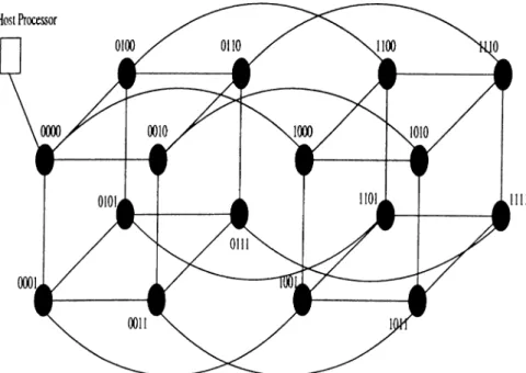
2.3 A 16 node hypercube m u ltic o m p u te r ... 25
2.4 (a) A ring embedding (b) A 2-dirnensional mesh embedding into a 4-dimensional hypercube... 26
2.5 The node algorithm in pseudo-code for patch circulation scheme... 29
2.6 The node algorithm in pseudo-code for form-factor computation by stor age sharing scheme... 30
2.7 Parallel G J algorithm... 33
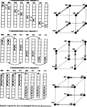
2.8 Global concatenate operation for a 3-dimensional hypercube... 34
2.9 Parallel S C G m ethod... 36
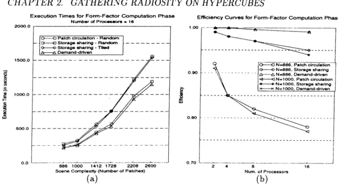
2.10 Form-factor computation phase, (a) Execution times for different schemes on 16 processors, (b) Efficiency curves for different schemes... 44
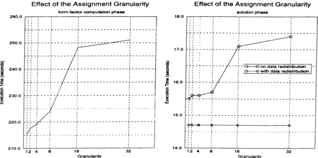
2.11 The effect of the assignment granularity on the performance (execution time in seconds) of the demand driven scheme for N = 886, P = 16. . . . 45
2.12 Efficiency curves for the S C G m ethod... 47
3.1 The polygon rendering pipeline... 51
3.2 A polygon with 5 vertices... 52
3.3 World and viewing coordinate systems... 53
3.4 The z-buffer array... 55
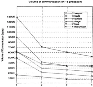
3.5 An e.xample of image-space parallelism. The screen is partitioned and subregions are assigned to processors (PO, P i, P2, P3)... 58 3.6 .Λη example of object-space parallelism... 59 4.1 Volume of communication on different meshes embedded on the hypercube
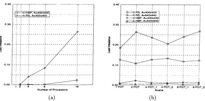
of 16 processors for different scenes... 84 4.2 Extended span algorithm... 90 4.3 Comparison of RS with HBP. (a) Different number of processors for 2
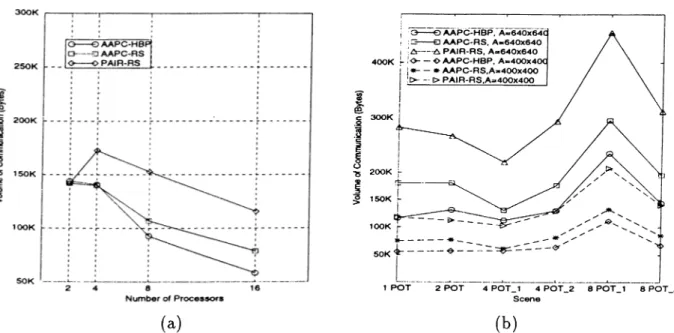
POT scene, A = 400 x 400. (b) Different screen resolutions and different scenes on 16 processors... 94 4.4 Volume of communication for (a) 2 POT scene on different processors,
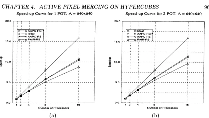
A = 400 X 400. (b) A = 400 x 400 and A = 640 x 640 for different scenes on 16 processors... 95 4.5 Speedup figures for A = 400 x 400. (a) 1 POT scene (b) 2 POT scene. 95 4.6 Speedup figures for A = 640 x 640. (a) 1 POT scene (b) 2 POT scene. 96 4.7 The Parsytec CC system... 97 4.8 Rendering rates of algorithms on Parsytec CC system, (a) A.APC-HBP
(b) ZBU F-EXC... 100 4.9 Speedup values achieved by the algorithms on Parsytec CC system, (a)
AAPC-H BP (b) ZBUF-EXC...100 4.10 Total volume of communication and concurrent volume of communication. 101 4.11 Rendered images of the scenes used in the experiments on iPSC/2. (a) 1
POT scene (b) 2 POT scene...102 4.12 Rendered images of the scenes used in the experiments on iPSC/2. (a) 4
POT-1 scene (b) 4 POT_2 scene... 102 4.13 Rendered images of the scenes used in the experiments on iPSC/2. (a) 8
POT-1 scene (b) 8 POT-2 scene... 103 4.14 Rendered images of the scenes used in the experiments on the Parsytec
CC system, (a) Teapot scene (102080 triangles, rendering time is 0.332 seconds on 16 processors) (b) Balls scene (157440 triangles, rendering time is 0.495 seconds on 16 processors). . ... 104
4.15 Rendered images of the scenes used in the experiments on the Parsytec CC system, (a) Lattice scene (235200 triangles, rendering time is 0.7 seconds on 16 processors) (b) Rings scene (343200 triangles, rendering time is 0.821 seconds on 16 processors)... 104 4.16 Rendered images of the scenes used in the experiments on the Parsytec CC
system, (a) Tree scene (425776 triangles, rendering time is 0.576 seconds on 16 processors) (b) Mountain scene (524288 triangles, rendering time is 1.052 seconds on 16 processors)... 105 5.1 A volumetric data set. Figure illustrates a 2-dimensional projection of
the volume, (a) Volume is sampled at 3-dimensional space. Each small filled circle represents the sample points with 3-dimensional spatial coor dinates. Dashed lines represent the boundaries of the volume, (b) Sample points are connected to form volume elements. A tetrahedral cell, which is formed by connecting four distinct sample points, is also illustrated. . . 108 5.2 Types of grids encountered in volume rendering...110 5.3 Ray-casting based direct volume rendering...I l l 5.4 Re-sampling phase of the ray-casting DVR. The color and opacity values
at the sample point on the ray are calculated by finding the contributions of original sample points which form the cell. After re-sampling, sample points on the ray are composited to generate the color on the screen. . . 113 6.1 An example of horizontal subdivision for eight processors...129 6.2 An example of rectangular division for 8 processors organized into 4 clus
ters and 2 processors in each cluster...131 6.3 -An example of recursive subdivision for eight processors... 132 6.4 An example of mesh-based adaptive hierarchical decomposition for eight
processors. Mesh resolution is 8 x 8... 136 6.5 Traversing of the 2-dimensional mesh with Hilbert curve and mapping of
the mesh cells locations into one-dimensional array indices... 137 6.6 An example of Hilbert curve based subdivision for eight processors. Mesh
6.7 An example of graph partitioning based subdivision for eight processors. Mesh resolution is 8 x 8...139 6.8 The algorithm to classify the primitives at redistribution step of HS, RS,
RRS, and MAHD algorithms...141 6.9 The algorithm to classify primitives in HCS and GS algorithms...142 6.10 Rendered images of the data sets used in the experiments, (a) Blunt fin
(381548 triangles, rendering timéis 6.27 seconds on 16 processors) (b) Post data (1040588 triangles, rendering time is 8.55 seconds on 16 processors). 143 6.11 Load balancing performance, based on the approximate load calculations,
of the MAHD, HCS, and GS algorithms (a) Different mesh resolutions on 16 processors, (b) Different number of processors... 144 6.12 Percent increase in the number of primitives after primitive redistribution.
Each value in the graph represents the percent increase in the total number of primitives for the mesh resolution the algorithm finds the best load balance, based on the estimated load distribution...145 6.13 Load balancing performance, based on the actual primitive distribution,
of the MAHD, HCS, and GS algorithms (a) Different rnesh resolutions on 16 processors, (b) Different number of processors... 146 6.14 Percent increase in the number of primitives after primitive redistribution.
Each value in the graph represents the percent increase in the total number of primitives for the mesh resolution the algorithm finds the best load balance, based on the actual distribution of primitives... 147 6.15 Execution time of MAHD, HCS, and GS for different mesh resolutions. . 148 6.16 Load balance performance of all algorithms (HS, RS, RRS, M.AHD, HCS,
and GS) on different number of p r o c e s s o r s ... 149 6.17 Percent increase in the number of primitives after redistribution for all
algorithms on different number of processors. Each value in the graph represents the percent increase in the total number of primitives for the mesh resolution the algorithm finds the best load balance, based on the actual distribution of primitives... 150
6.18 Execution time of all algorithms on different number of processors. For MAHD, HCS, and GS algorithms, the values represents the execution time of the respective algorithm for the mesh resolution the algorithm achieves the best load distribution... 151 6.19 Speedup for only rendering phase when only the number of triangles in a
region is used to approximate work load in a region... 158 6.20 Speedup for rendering phase (step 4 of the parallel algorithm) when spans
and pixels are incorporated into the subdivision algorithms... 158 6.21 Speedup values including the e.xecution time of subdivision algorithms. . 159 6.22 Errors due to bounding box approximation in calculating the number of
spans when vertical divisions are allowed...159 6.2.3 Rendering times in seconds, (a) Only rendering time excluding subdivision
2.1 Relative performance results in parallel execution times (in seconds) of different parallel algorithms for the form-factor computation phase. N is the number of patches in the scene and M is the number of non-zero entries in the form-factor matrix... 43 2.2 Parallel execution times (in seconds) of various schemes in the solution
phase (using G J ) along with the associated overheads. T O T is the total execution time including overheads, i.e. T O T = (solution + preprocess ing) time. N is the number of patches in the scene and M is the number of non-zero entries in the form-factor matrix... 46 2.3 Performance comparison of parallel Gauss-Jacobi and Scaled
Conjugate-Gradient methods (1* denotes the estimated sequential timings). Timings are in seconds. N is the number of patches in the scene and M is the number of non-zero entries in the form-factor matrix... 49 4.1 Scene characteristics in terms of total number of pi.xels generated (T P G ),
number of triangles, and total number of winning pi.xels in the final picture (T P F ) for different screen sizes... 91 4.2 Relative execution times (in milliseconds) of full z-buffer merging and
PAIR-RS for N=400... 92 4.3 Comparison of execution times (in milliseconds) of several pi.xel merging
schemes... 93 4.4 Number of triangles in the test scenes... 96
6.1 Dissection of execution time of each algorithm on different number of processors... 148
Introduction
Rendering in computer graphics can be described as the process of generating a 2- dirnensional representation of a data set defined in 3-dimensional space. Input to this process is a set of primitives defined in a 3-dimensional coordinate system, usually called world coordinate system, and a viewing position and orientation also defined in the same world coordinate system. The primitives are objects, polygons, surfaces, or points con nected in a predetermined way (as in volumetric data sets), which constitute the input data set. The viewing position and orientation define the orientation and location of the image-plane, which represents the computer screen. The output of the rendering process is a 2-dimensional picture of the data set on the computer screen. Figure 1.1 illustrates an example of computer graphics rendering with its input and output.
In this thesis, we investigate the utilization of distributed-rnernory multicomputers in three different fields of computer graphics rendering:
Realistic simulation o f light propagation: One of the challenging fields in computer graphics rendering is to model the light-object interactions and propagation of light in an environment realistically. Ray tracing [102] and radiosity [33] are two popular methods used in such applications. The target method in this thesis is the gathering radiosity [33] method.
Polygon rendering: Algorithms and methods in polygon rendering field deal with producing realistic images of computer generated environments com posed of polygons.
The world coordinate system
Figure 1.1: An example of computer graphics rendering.
Volume rendering: Volume rendering techniques deal with visualization of scientific data sets composed of large amounts of numerical data values asso ciated with points in 3-dimensional space. This thesis investigates methods for parallel rendering of unstructured grids, in which points are irregularly distributed in 3-dimensional space.
Realistic illumination models and shading methods, like gathering radiosity, require large memory space and computing power. Moreover, increased complexity of computer generated environments has added more memory space and more computing power re quirements in polygon rendering. Similarly, techniques applied in volume rendering and huge size o f data sets obtained in scientific applications require large memory space and high computing power. It is unlikely to meet increasing reciuirements of these fields on single processor machines with today’s technology, whereas distributed-memory multi computers can provide a cost-effective solution. Large memory space and high computing power requirements are met by connecting many processors with individual memories and using these processors simultaneously. Each processor in the architecture can per form computations asynchronously on different data values, thus providing a flexible
environment. Flexibility provides a cost-effective working environment for many appli cations of different nature and characteristics. Distributed-memory multicomputers can be upgraded and extended by adding more processors with individual memories to the environment, thus providing a scalable environment. Scalability provides an inherent power to meet increasing requirements of the applications. As the name implies, there is no shared global memory in distributed-memory architectures. Each processor has its owm local memory, which cannot be directly accessed by other processors. Synchroniza tion and data exchange between processors are carried out via exchanging messages over an interconnection network. Among many interconnection topologies, rings, meshes, hypercubes, and multistage switch based networks are the most commonly used network topologies.
In this chapter, brief overviews of gathering radiosity, polygon rendering, and vol ume rendering are given. Following the overviews, contributions of the thesis work are presented. Organization of the thesis is given in the last section.
1.1
Gathering Radiosity
Given a description of the environment, producing a realistic image of the environment on the computer is accomplished in three basic steps; (1) - reading the description o f the environment and converting the description into appropriate form to apply rendering algorithms, (2) - simulating the propagation o f light in the environment, (3) - displaying the environment on the computer screen.
At the first step, the description of the environment to be rendered is read into the computer. The description of the environment is converted into appropriate form that is suitable for algorithms to simulate light propagation and to display the environment. For e.xarnple, surfaces and objects descriptions should be converted into polygons to apply polygon rendering algorithms.
Next step is to simulate the propagation of light in the environment and light-object interactions. Various methods are used in computer graphics rendering [95, 96, 77]. Simple methods, such a.s Phong method [68], only simulate the interaction of light, com ing directly from light sources, with the objects in the environment. These methods
result in moderate realism in the images because the contributions of light reflected from other objects in the environment are not considered. More realistic and complex methods account for the reflected and refracted light as well. There are two methods, called ray tracing [102] and radiosity [.33], which are widely used for accurately simulating propagation of light in an environment.
The radiosity method accounts for the diffuse inter-reflections between the surfaces in a diffuse environment. There are two approaches to radiosity, progressive refinement [L5] and gathering [33] methods. Gathering is a very suitable approach for investigating lighting effects within a closure. In this method, every surface and object constituting the environment is discretized into small patches (polygons), which are assumed to be perfect diffusers. The algorithm calculates the radiosity value of each patch in the scene. Initially, all patches, except for light sources, have zero initial radiosity values. The light sources are also treated as patches. The algorithm consists of three successive computational phases: form -factor computation phase, solution phase and rendering phase.
The form-factor matrix is computed and stored in the first phase. In an environment discretized into N patches, the radiosity bi of each patch “i’’ is computed as follows:
N
b, = e,· + ri bjF,j j=i
(1.1)
where e, and r, denote the initial radiosity and reflectivity values, respectively, of patch “i” and the form-factor F,j denotes the fraction of light that leaves the patch “i” and incident on patch “j ” . The value of F,j depends on the geometry of the scene and it is constant as long as the geometry of the scene remains unchanged. The Fa values are taken to be zero for convex patches. This linear system of equations can be represented in matrix form as follows
C b = ( I - R F ) b = e (1.2)
where, R is the diagonal reflectivity matrix, b is the radiosity vector to be calculated, e is the vector representing the self emission (initial emission) values of patches, and F is the form-factor matrix.
In the second phase, a linear system of equations is solved for each color-band (e.g. red, green, blue) to And the radiosity values of all patches for these colors. In the last
phase, results are rendered and displayed on the screen using the radiosity values of the patches computed in the second phase. The radiosity values are transformed into color values for shading the polygons. Conventional polygon rendering methods [95, 77] (e.g. Gouraud shading, z-buffer algorithm) are used in the last step to display the results.
1.2
Polygon Rendering
.A.S noted in the previous section, the last step of realistic image generation is to dis
play the environment on the computer screen. A pipeline of operations is applied to transform polygons from 3-dirnensional space to 2-dimensional screen space, perform smooth shading of the polygons, and perform hidden-surface removal to give realism to the image produced. Light-polygon interactions and shading of the polygons can also be done concurrently with hidden-surface removal if simple methods to calculate light- object interactions are used. Hidden-surface removal is a kind of sorting operation [86] to determine the visible parts of the polygons. Polygons are sorted by their distance to the screen. The overhead of sorting is decreased by utilizing some kind of coherency existing in the environment. Among many algorithms, z-buffer and scanline z-buffer algorithms are more popular due to wider range of applications and better utilization of coherency. These algorithms are called image-space algorithms since hidden-surface removal, hence sorting, is performed at pixel locations on the screen. In order to ac complish this, polygons are projected onto the screen and distance values are generated for screen coordinates covered by the projection of the polygon. Hidden-surface removal at a pixel location is done by comparing the distance values generated at the pixel lo cation. These algorithms utilize image-space coherency to calculate the distance values at pixel locations. Calculation of distance value from one pixel to the next is done via incremental operations.
1.3
Volume Rendering
Visualization of scientific data aims at displaying vast amount of numerical data ob tained from engineering simulations or gathered by scanning real physical entities by
advanced scan devices. Visualization of volumetric data sets, in which numerical values are obtained at sample points with 3-dimensional spatial coordinates in a volume, is referred to here as volume rendering. Sample points in these sets form a 3-dimensional grid superimposed on the volume. In this grid, sample points are connected to other sample points in a predetermined way to form volume elements, referred to here cis cells. A sample point may be shared by many cells. In addition, a cell may share a face with other cells, forming a connectivity relation between volume elements. In volumetric data sets, two types of grids are commonly encountered. In structured grids, the sample points are regularly distributed in the volume. There exists implicit and regular connectivity between volume elements. This type of grids are most common in medical imaging ap plications. In unstructured grids, the sample points are distributed irregularly in the 3-dimensional space. There exists irregular connectivity between volume elements if a connectivity relation exists at all. Unstructured grids are commonly used in engineering simulations (e.g., computational fluid dynamics).
Volumetric data sets are rendered by finding the contribution of sample points to the pixels on the screen. These contributions are determined via processing the volume elements. Each of these contributions are transformed into color values to display the volume. Among many techniques in volume rendering, ray-casting based direct volume rendering [54, 92], which is the basis of research on parallel volume rendering in this the sis, has become very popular. Direct volume rendering (DVR) describes the process of visualizing the volume data without generating an intermediate geometrical representa tion such as isosurfaces. In ray-casting based direct volume rendering, rays are cast from pixel locations and traced in the volume. During the traversal in the volume, sample points are taken along the ray. The contribution of the volume element that contains the sample point is calculated. Then, these values at each sample point on the ray are composited in a predetermined order (front-to-back or back-to-front) to obtain the con tribution at the pixel. Determining the volume element that contains the sample point is called point location problem and compositing the contributions in a predetermined order is called view sort problem. Resolving point location and view sort problems is a crucial issue that closely affects the performance of the rendering algorithm. Handling
point location and view sort problems in structured grids are easy due to regular distri bution of sample points and implicit regular connectivity between volume elements. On the other hand, irregular distribution of sample points and irregular connectivity relation between volume elements (if it exists) make the point location and view sort problems much more difficult to handle in unstructured grids.
Application of Polygon Rendering Algorithms in Volume Rendering
Although polygon rendering and volume rendering form two diverse application areas of computer graphics in many aspects, techniques and algorithms used in one field can easily be adapted to resolve the problems in the other field.
As is stated, ray-casting based direct volume rendering algorithms should resolve the point location and view sort problems efficiently as these problems affect the perfor mance directly. In many application, these problems reduce to finding the intersection of ray with respective volume elements. These intersections are then sorted in increasing distance from the screen so that composition of contributions of sample points is done correctly.
In polygon rendering, image-space hidden-surface removal algorithms such as z-buffer and scanline z-buffer actually perform a similar sorting of the object database to perform hidden-surface removal correctly. In addition, polygons are rasterized (or scan-converted) to generate color and distance values for the pixels covered by the polygon. This raster ization corresponds, in a sense, to finding the intersection of the polygon with the rays cast from those pixel locations. Image-space hidden-surface removal algorithms utilize image-space coherency to decrease the overheads of sorting and rasterization. Such a co herency also exists in ray-casting based DVR applications. Therefore, ray-casting based DVR can benefit from the application of polygon rendering algorithms since the basic problems are almost the same.
1.4
Contributions of the Thesis
In this thesis, utilization of distributed memory multicomputers in three fields, which are gathering radiosity, polygon rendering and volume rendering, in computer graphics
is investigated. This section presents the contributions of the thesis work.
1.4.1
Parallel Gathering Radiosity
Parallelization of form-factor matrix computation and solution phases of the gathering radiosity are the key issues in this work. The contributions of the thesis work in these issues are the following.
• In parallel computation of the form-factor matrix, several algorithms were devel oped. Interprocessor communication is decreased by sharing the memory space between matrix elements and the objects in the scene. A demand-driven algorithm is proposed to achieve better load balance among processors in form-factor com putations. Our demand-driven approach is different from [12, 13]. Unlike their approach, we avoid re-distribution of matrix rows after matrix is calculated by not doing a conceptual partitioning of patches among processors. However, our scheme necessitates two-level indexing in matrix-vector product operations in the solution phase. A parallel re-numbering scheme is proposed to eliminate two-level indexing. • All previous works used Gauss-Jacobi (G J ) iterative algorithm in the solution
phase. We apply more efficient Scaled Conjugate-Gradient (S C G ) algorithm in the solution phase. The non-symmetric coefficient matrix is converted to a symmetric matrix to apply S C G . This conversion is done without perturbing the sparsity structure of the matrix.
• Parallel algorithms were developed for G J and S C G algorithms for hypercube- connected multicomputers. In order to achieve better load balance in the solution phase, an efficient data redistribution scheme is proposed. This scheme achieves perfect load balance in matrix-vector product operations in the solution phase. We obtain high efficiency values in the solution phase using S C G with data redistri bution.
1.4.2
Parallel Polygon Rendering
Object-space parallelism (Section 3.2.1) is investigated for parallel polygon rendering on hypercube-connected multicomputers. Briefly, in object-space parallelism, scene data is partitioned into disjoint sets among processors. Each processor performs the rendering of its local partition of primitives. This phrise of rendering is referred to as local rendering phase. Then, full screen partial images in each processor are merged to obtain the final image. This phase is called pixel merging phase. The pixel merging phase necessitates interprocessor communication to merge partial images. In this work, hypercube inter connection topology and message passing structure is exploited in pi.xel merging phase. The contributions in this thesis are the following.
• Volume of communication in pixel merging phase is decreased by only exchanging local foremost pixels in each processor after local rendering phase.
• A modified scanline z-buffer algorithm is proposed for local rendering phase. The nice features of this algorithm are: It avoids message fragmentation by storing local foremost pixels in consecutive memory locations efficiently. In addition, it elimi nates initialization of scanline z-buffer for each scanline on the screen. Initialization o f z-buffer introduces a sequential overhead to parallel rendering.
• For pixel merging phase, we propose two schemes referred to here as pairwise ex change scheme and all-to-all personalized communication (.A.4PC) scheme, which are suited to the hypercube topology. Pairwise exchange scheme involves mini mum number of communication steps, but it has memory-to-memory copy over heads. All-to-all personalized communication scheme eliminates these overhead by increasing the number of communication steps. Our AAPC scheme differs from 2- phase direct pixel forwarding of Lee [53]. Our algorithm is 1-phase algorithm, i.e., pixels are transmitted to destination processors in a single communication phase. Hence, our algorithm avoids the intermediate z-buffering in [53] totally.
• All of the processors are utilized actively throughout the pixel merging phase by exploiting the interconnection topology of hypercube and by dividing the screen among processors.
• We investigate load balancing in pixel merging phase. Two heuristics, recursive subdivision and heuristic bin packing, were proposed to achieve better load bal ancing in pixel merging phase. These heuristics are adaptive in that they utilize the distribution of foremost pixels on the screen to subdivide the screen for the pixel merging phase.
Most of the research work was performed on Intel’s iPSC/2 hypercube multicom puter. Recently, the AAPC scheme with heuristic bin packing algorithm was ported to Parsytec’s CC system with PowerPC processors. In the current implementation, a hypercube topology is assumed and the topology of CC system is not exploited. Our pre liminary results on the CC system achieves rendering rates of 300K - TOOK triangles/sec on 16 processors.
An earlier version of the parallel polygon rendering work appears in [51].
1.4.3
Parallel Volume Rendering
In volume rendering field, image-space parallelism (Section 3.2.1) for parallel volume rendering of unstructured grids is investigated. In image-space parallelism, the screen is subdivided into regions. Each processor is assigned one or more subregions. The primi tives (e.g., tetrahedrals) in the volume data are distributed among processors according to screen subdivision and processor-subregion assignments. Then, each processor renders its local subregions. The contributions in this thesis are the following.
• Main topic in this work is the adaptive subdivision of screen for better load balance. Adaptive subdivision issue has not been investigated before in parallel volume ren dering o f unstructured grids. Only some researchers utilized adaptive subdivision in parallel polygon rendering [76, 99, 65, 26] and in ray tracing/casting [5]. The algorithms presented in this work can be grouped into two classes: 1-dimensional array based algorithms and 2-dimensional mesh based algorithms.
• Among the 2-dimensional mesh based algorithms, graph partitioning based sub division and Hilbert curve based subdivision algorithms are new approaches in parallel rendering.
• An experimental comparison of the subdivision algorithms is performed on a com mon frame work.
• The subdivision heuristics are employed in parallelization of a volume rendering algorithm. The sequential volume rendering algorithm is based on Challinger’s work [9, 10]. This algorithm is basically a polygon rendering based algorithm. It requires volume elements composed of polygons and utilizes a scanline z-buffer approach to resolve point location and view sort problems. In the previous works on parallel polygon rendering, only the number of primitives in a subregion were used to approximate the work load of the subregion. We experimentally show that this approximation is not enough. Better speedup values can be obtained by utilizing other criteria such as number of pixels and number of spans in a region. By utilizing these additional criteria, the speedup values are almost doubled.
An earlier version of the parallel volume rendering work is published in [89].
1.5 Organization of the Thesis
The rest of the thesis is organized as follows.In Chapter 2, parallel implementation of form-factor computation and solution phases of gathering radiosity on hypercube-connected multicomputers is presented. A brief description of iPSC/2 hypercube multicomputer, an overview of gathering radiosity and previous work on parallel gathering radiosity are also included in this chapter.
Chapter 3 presents an overview of sequential polygon rendering. In addition, a tax onomy o f parallelism in polygon rendering is introduced. Previous works, classified with respect to this taxonomy, are summarized in this chapter.
In Chapter 4, an object-space parallel algorithm for polygon rendering on hyper cube multicomputers is presented. Several schemes for efficient implementation of local rendering and pixel merging phases are described.
An overview of volume rendering for unstructured grids is presented in Chapter 5. Previous works on parallel volume rendering of unstructured grids are summarized in this chapter.
Spatial subdivision algorithms, developed in this thesis, for image-space parallel vol ume rendering are described in Chapter 6.
Gathering Radiosity on Hypercubes
Realistic synthetic image generation by computers has been a challenge for many years in the computer graphics field. Realistic synthetic image generation requires the accurate calculation and simulation of light propagation and global illumination effects in an environment. The radiosity method [33] is one of the techniques to simulate the light propagation in a closed environment. Radiosity accounts for the diffuse inter-reflections between the surfaces in a diffuse environment. There are two approaches to radiosity, progressive refinement [15] and gathering [33] methods. The gathering method (the term radiosity method will also be used interchangeably to refer to gathering method) consists of three successive computational phases: form -factor computation phase, solution phase and rendering phase. The form-factor matrix is computed and stored in the first phase. In the second phase, a linear system of ecjuations is formed and solved for each color-band (e.g. red, green, blue) to find the radiosity values of all patches for these colors. In the last phase, results are rendered and displayed on the screen using the radiosity values of the patches computed in the second phase. Conventional rendering methods [95, 77] (e.g. Gouraud shading, z-buffer algorithm) are used in the last phase to display the results.
Gathering is a very suitable approach for investigating lighting effects within a closed environment. For such applications, the locations of the objects and light sources in the scene usually remain fixed while the intensity and color of light sources and/or reflectiv ity of surfaces change in time. The linear system of equations are solved many times to
investigate the effects of these changes. Therefore, efficient implementation of the solu tion phase is important for such applications. Although gathering is excellent for some applications in realistic image generation, it requires high computing power and large memory storage to hold the scene data and computation results. As a result, applica tions of the method on conventional uniprocessor computers for complex environments can be far from being practical due to high computation and memory costs.
In this chapter, parallelization of the first two phases of the gathering method is inves tigated for hypercube-connected multicomputers. In parallel computation o f form-factor matrix, several algorithms were developed. Interprocessor communication is decreased by sharing the memory space between matrix elements and the objects in the scene. A demand-driven algorithm is proposed to achieve better load balance among processors in form-factor computations. Our demand-driven approach is different from [T2, 13]. We do not perform a conceptual partitioning of patches among processors. Thus, matrix rows are not redistributed after the matrix is calculated. However, our scheme necessi tates two-level indexing in matrix-vector product operations in the solution phase. .An efficient parallel re-numbering scheme is proposed to eliminate the two-level indexing.
The previous works [12, 13, 67, 73] utilized Gauss-.Jacobi (G J ) iterative algorithm in the solution phase. We apply the more efficient Scaled Conjugate-Gradient (SC G ) algorithm in the solution phase. The non-symmetric coefficient matrix is converted into a symmetric matrix to apply S C G . This conversion is done without perturbing the sparsity structure of the matrix. Parallel algorithms were developed for G J and SC G algorithms for hypercube-connected multicomputers. In addition, load balancing in the solution phase is investigated. An efficient data redistribution scheme is proposed. This scheme achieves perfect load balance in matrix-vector product operations in the solution phase. We obtain high efficiency values in the solution phase using S C G with data redistribution.
The organization of this chapter is as follows. Section 2.1 describes the computational requirements and the methods used in the form-factor computation and solution phases. The proposed S C G algorithm is described in this section as well. Section 2.2 briefly summarizes the existing work on the parallelization of the gathering radiosity method. Section 2.4 presents the parallel algorithms developed for the form-factor computation
phase. The parallel algorithms developed for the solution phcise are presented and dis cussed in Section 2.5. Load balancing in the solution phase and a data redistribution scheme are discussed in Section 2.6. Finally, experimental results on a 16-node Intel iPSC /2 hypercube multicomputer are presented and discussed in Section 2.7.
2.1
Gathering Radiosity
Radiosity is based on the energy equilibrium within a closure. In this method, every surface and object constituting the environment is discretized into small patches. Each patch is assumed to be a perfect diffuser or an ideal Lambertian surface. The algorithm calculates the radiosity value of each patch in the scene. The radiosity value of a patch is defined to be the amount of light leaving that patch in equilibrium state. It is a function of emitted and reflected light from the patch. Initially, all patches have zero initial radiosity values. The light sources are also treated as patches except they possess non zero initial radiosity values. In an environment discretized into N patches, the radiosity 6, of each patch “i” is computed as follows:
N
bi = e. + r, bjF,^ (2 . 1)
where e, and r; denote the initial radiosity and reflectivity values, respectively, of patch "i” and the form-factor Fij denotes the fraction of light that leaves the patch “i” and incident on patch “j ” . The value of Fq depends on the geometry of the scene and it is constant as long as the geometry of the scene remains unchanged. This linear system of equations can be represented in matrix form as follows:
l - r i F n -I'lF n -^2^21 1 - T2F22 -r^vF/vi - tnFm2 -riFiN ■f’2F2N ' ' ei «2 b]^ . e/v _
(2.2)
1 — rf^F^NThe Fa values are taken to be zero for convex patches. Assuming F„ = 0, the coefficient matrix in Eq. (2.2) can further be decomposed into three matrices as
1 0 0 . .. 0 ^1 0 0 0 0
F n
F i 3 . .. F i ; v 0 1 0 . .. 0 0 ^2 0 0F21
0F
2 3 ..F
2N
0 0 1 .,.. 0 0 0 ^3 . .. 0
F
3 1F
3 2 0 . ..F 3
n0 0 0 .... 1 0 0 0 .
F
n iF
n2 F m
·· . 0I R
Hence, Eq. (2.2) can be re-written as follows:
C b = ( I - R F ) b = e (2.3)
where, R is the diagonal reflectivity matrix, b is the radiosity vector to be calculated, e is the vector representing the self emission (initial emission) values of patches, and F is the form-factor matrix.
2.1.1
Form-Factor Computation Phase
An approximate method to calculate the form-factors is proposed in [16], called the hemi-cube method. In this method, a discrete hemi-cube is placed around the center of a patch. Each face of the hemi-cube is divided into small squares (surface squares). A typical hemi-cube is composed of 100x100x50 such scfuares. Each square “s” corresponds to a delta form-factor ( A /( s ) ) , which is a function of the area of the square, and the displacement of the square in x,y or y,z directions depending on the square “s” being located on the top face or side faces of the hemi-cube, respectively.
After allocating a hemi-cube over a patch “i” , all other patches in the environment are projected onto the hemi-cube for hidden patch removal. The patches are passed through a projection pipeline consisting of visibility test, clipping, perspective projection, and scan conversion. This projection pipeline is analogous to a z-bufFer algorithm except for the fact that patch numbers are recorded for each allocated hemi-cube surface square in addition to z values. Then, each square “s” allocated by patch “j ” contributes A /( s ) to the form-factor Fij between patches “i” and “j ” . At the end of this process row of the form-factor matrix F is constructed. This process is repeated for all patches in the
environment in order to construct the whole F matrix. Sum of the form-factor values in each row o f the F matrix is equal to 1 by definition.
The F matrix is a sparse matrix because a patch does not see all the patches in the environment due to the occlusions. Almost 60%-85% of the F matrix elements are observed to be zero in the test scenes. In order to reduce the memory requirements, F matrix is stored in compressed form. Space is allocated for only non-zero elements of the matrix dynamically during the form-factor computation phase. Each element of a row of the matrix is in the form [column-id,value]. The column-id indicates the _/index o f an Fij value in the row.
2.1.2
Solution Phase
In this phase, the linear system of equations (Eq. (2.3)) is solved for each color-band. Methods for solving such linear system of equations can be grouped as direct methods and iterative methods. Direct methods such as Gaussian elimination and LU factoriza tion [32] disturb the original sparsity of the coefficient matrices during the factorization. Furthermore, direct methods necessitate maintaining a coefficient matrix and two fac tor matrices for each color matrix for lighting simulations. As a result, direct methods require excessive memory for the solution phase of the radiosity method.
Iterative methods start from an initial vector
b®
and iterate until a predetermined convergence criterion is reached. The sparsity of the coefficient matrix is preserved through out the iterations. Maintaining only the form-factor matrix F suffices in the for mulations o f the iterative methods proposed in this w'ork. Experimental results demon strate that iterative methods converge quickly to acceptable accuracy values in the so lution phase o f the radiosity method. Furthermore, iterative methods are in general more suitable for parallelization than direct methods. Hence, direct methods are not considered in this work.Three popular iterative methods widely used for solving linear system of equations are Gauss-Jacobi (G J ). Gauss-Seidel (G S ), and Conjugate-Gradient (C G ) [32]. The computational complexity of a G S iteration is exactly equal to that of G J scheme. In general, G S scheme converges faster than the G J scheme. Unfortunately, the GS scheme is inherently sequential and hence it is not suitable for parallelization. Thus, only GJ
and C G schemes are described and investigated for parallelization in this work.
G a u s s -J a c o b i M e t h o d
In the G J method, the coefficient matrix C is decomposed a s C = D — L — U where D, L and U are the diagonal, lower triangular and upper triangular parts of C respectively. Then, the iteration equation can be represented in matrix notation as
b^+i = D " ‘ ((L + U)b*^ + e). (2.4) Since C = I - R F and Fa = 0 for all i = 1,2,...,N, we have D = I and L + U = R F . Hence, the iteration equation for the solution phase of the radiosity becomes
b^+i ^ R F b* + e. (2.5)
Recalling that the linear system of equations is to be constructed and solved for each color band, the G J iteration eciuations for different colors can be re-written as
= R{<',g,l>)Fh’‘ {r,g,b) + e {r,g ,b ). (
2
.6
)Note that, it suffices to store only the diagonals of the diagonal R matrix. Hence, matrix and vector will be used interchangeably to refer to diagonal matrix. Therefore, Eq. (2.6) clearly illustrates that the G J algorithm necessitates storing only the original F matrix and the reflectivity vector for each color in the solution phase. In order to minimize the computational overhead during the iterations due to this storage scheme, the matrix product R F , which takes 0 (A /) time, should be avoided in the implementation, where M denotes the total number of non-zero entries in the F matrix. That is, the first term in the right-hand-side of the Eq. (2.5) should be computed as a sequence of two matrix- vector products X = F b and R x , which take Q {M ) and 0(A^) times, respectively. Since M = O(N ^) is asymptotically larger than N, this computational overhead is negligible. The algorithm for G J method is given in Fig. 2.1. The computational complexity of an individual G J iteration is
T G j ^ i 2 M + 6N)Catc. (2.7)
Here, scalar addition, multiplication and absolute value operations are assumed to take the same amount of time
tcaic-Initially, choose b° for k = 1,2,3,...
1. form =, R F b * + e as
X = Fb*^ ; y = Rx ; b^+' = y + e
2. r* = b*^+‘ - b^
3. check Norm (r*')/m ax(b*) < e
where Norm(r*) = |rf| and max{h^) = max{\b'-\)
Figure 2.1: Basic steps of the G J method.
The convergence of the G J method is guaranteed if the coefficient matrix is diagonally dominant. In radiosity, the coefficient matrix C = I — R F satisfies diagonal dominance since Fij — 1, Fa - 0 and 0 < r; < 1 (for each color band) for each row “i” .
S ca led C o n ju g a te -G r a d ie n t M e th o d
The C G method [39] is an optimization technique, iteratively searching the space of vectors b to minimize the objective function / ( b ) = 1/2 < b ,C b > — < e, b > where b = [6 i...., 6,v]/ / : R^ R and < ·, · > denotes the inner product of two vectors. If the coefficient matrix C is a symmetric and positive-definite matrix the objective function defined above is a strictly convex function and has a global minimum where its gradient vector vanishes, i.e. = C b — e = 0, which is also the solution to Eq. (2.3). The C G algorithm seeks this global minimum by finding in turn the local minima along a series o f lines, the directions of which are given by vectors po, p i , ... in an N-dimensional space.
As is mentioned earlier, the convergence of the C G method is guaranteed only if the coefficient matrix C is symmetric and positive-definite. However, the original coefficient matrix is not symmetric since c,j = r,F,j ^ TjFji — cji. Therefore, the C G method cannot be used in the solution phase using the original C matrix as is also mentioned in [67]. However, the reciprocity relation A{Fij = between the form factor values of the patches can be exploited to transform the original linear system of equations in
Eq. (2.3) into
Sb = De (2.8)
with a symmetric coefRcient matrix S = DC where D is a diagonal matrix D = diag[Ai/ri, A2/t2, ■■■, Ai>i/ri^]. Note that matrix S is symmetric since = A{Fij =
AjFji — Sji for j ^ i. The row of the matrix S hcis the following structure Sim — [ A i F i i , , Ai/vi, A { F i ^ i ^ i , AiEiTv]
for i — 1 ,2 ,..., N. Therefore, matrix S preserves diagonal dominance since Fij = 1 and 0 < < 1 (for each color band) for each row “i” . Thus, the coefficient matrix
S in the transformed system of equations (Eq. (2.8)) is positive-definite since diagonal dominance of a matrix ensures its positive-definiteness.
The convergence rate of the CG method can be improved by preconditioning. In this work, simple yet effective diagonal scaling is used for preconditioning the coefficient matrix S. In this preconditioning scheme, rows and columns of the coefficient matrix S
are individually scaled by its diagonal D = dia^[y4i/ri,..., Tyv/r^]. Therefore, the CG
algorithm is applied to solve the following linear system of equations
Sb = e (2.9)
where S = = D -i/^D C D -'/^ ^ d '/^ C D -'/^ has unit diagonals, b = D^/^b and e = Thus, the right-hand side vector D e in Eq. (2.8) is also scaled and b must be scaled back at the end to obtain the original solution vector b
(i.e. b = D-'/^b). The eigenvalues of the scaled coefficient matrix S (in Eq. (2.9)) are more likely to be grouped together than those of the unsealed matrix S (in Eq. (2.8)), thus resulting in a better condition number.
The entries of the scaled coefficient matrix S are of the following structure:
Sij — <
Fij if i 7^ j
otherwise.
The values of the scaling parameters v/r,vl,· and \JrjlAj depend only on the area and reflectivity values of the patches and do not change throughout the iterations. Therefore,