EFFECTS OF THE REAL EXCHANGE RATE ON OUTPUT
AND INFLATION: EVIDENCE FROM TURKEY
HAKAN BERUMENT
MEHMET PASAOGULLARI
This paper assesses the effects of real depreciation on the economic performance of Turkey by considering quarterly data from 1987:I to 2001:III. The empirical evidence suggests that, contrary to classical wisdom, the real depreciations are contractionary, even when external factors like world interest rates, international trade, and capital flows are controlled. Moreover, the results obtained from the analyses indicate that real ex-change rate depreciations are inflationary.
I. INTRODUCTION
HE1995 Mexican Tequila and the 1997 Asian crises have stimulated a growing
interest among academics and policymakers on the controversial issue of ex-change rate policies in general and exex-change rate regimes and real exex-change rates in particular. The effects of financial crises on the global economy are getting more severe, and international trade and capital movements have begun to be central factors in the evolution of such a crisis. Domestic factors that lead to crises in vari-ous countries are different, but there are also common features of these crises: big devaluations or depreciations in domestic currency and the subsequent significant output losses of the crisis-hit countries.
Turkey has often experienced financial crises in its history. In 1994 and 2001, the nominal domestic currency depreciated 62 per cent and 53 per cent, respectively. This made the effects of large depreciations an interesting event to study and also provided a natural laboratory where the effect of depreciation on economic perfor-mance could be observed. Starting in 1987, in a managed float exchange rate regime, the Central Bank of the Republic of Turkey (hereafter, the CBRT) an-nounced daily quotations, and the domestic currency was depreciated continuously parallel to inflation expectations. However, when there was considerable market pressure in times of crisis, large devaluations occurred. As in the case of the Asian and Mexican crises, common features, such as large devaluations or high levels of
T
We would like to thank Anita Akkas and the anonymous referees of the journal for their helpful com-ments.
depreciation in domestic currency and significant output losses, were experienced after both the 1994 and the 2001 crises. In 1994, output declined by 6.2 per cent after the financial crisis and sharp devaluation.
However, between these two severe financial crises, the Turkish economy exhib-ited strong performance on the output side, and the average growth of output be-tween 1995 and 1999 was 4.2 per cent, despite the detrimental effects of the 1998 Russian crisis, the two earthquake catastrophes and the recession that took place in 1999. During the 1995–99 period, the real exchange rate, defined as the nominal ex-change rate deflated by the wholesale price index, was relatively stable and there were times when sizeable capital inflow entered Turkey. With the Year 2000 Dis-inflation Program, the exchange rate regime was shifted from a managed float to a crawling peg regime. With the implementation of this program, a remarkable growth in the GDP and decline in inflation were seen, but the real exchange rate began to appreciate because of the differential between inflation and the preannounced change in the path of nominal exchange rates. However, after the banking and resulting liquidity crisis in November of 2000 and the serious attack on foreign change reserves in February of 2001, Turkish authorities decided to switch the ex-change rate regime to a floating regime. As expected, the exex-change rate surged and there was excessive volatility in the nominal exchange rate even after the first six or seven months of the crisis. Output responsed detrimentally to the large depreciation of the domestic currency and the real GNP and the real GDP declined by 9.4 per cent and 7.4 per cent, respectively, in 2001. The level of output performances was approximately the same as in 1997, indicating a decline in the welfare level of the Turkish public to the levels of four years before.
The 1994 and 2001 crises had different origins and different characteristics; how-ever, the crises also have common elements: namely, huge exchange rate deprecia-tion, preceding and/or coupled with capital outflows, preceding current account deficits, output declines, and high interest rates. There was a sizeable increase in the current account deficit preceding the crisis in 1993, and domestic currency was de-valued by more than 62%in nominal terms and 12.1% in real terms after the crisis. Similarly, in 2000, the year preceding the crisis, there was a considerable current ac-count deficit of approximately 4.9% of GDP. The Turkish lira depreciated by 53% in nominal terms and by 11.9% in real terms in 2001. In addition to these facts, output declined severely after both of the devaluations. The output responses after the great devaluations or depreciations suggest that the Turkish case constitutes a possible ex-ample of the contractionary devaluation hypothesis, and in this study we basically aim to find empirical support for this suggestion. This study mainly uses the method proposed by Kamin and Rogers (2000), which found empirical evidence for con-tractionary devaluation in the case of Mexico by analyzing the output and inflation response to real exchange rate movements.
ex-change rate on a quarterly basis. As seen in the figure, large devaluations are cou-pled with large declines in output, and appreciations are coucou-pled with growth in out-put. The figure suggests a negative relationship between those two variables. In this paper, we will investigate this negative correlation. However, before proceeding fur-ther, we have to say that the findings of this study will be carefully considered. For example, a finding that supports a view contradictory to the contractionary devalua-tion hypothesis may not recommend keeping the domestic currency at highly com-petitive levels because of the inflationary effects of such an action; or a finding that supports the contractionary devaluations hypothesis may not be implemented be-cause of the higher risk of financial crisis in the presence of an overvalued domestic currency, when the 1994 and 2001 cases are taken into consideration. However, this study aims mainly at showing the output and inflation responses after the devalua-tion.
The importance of this study is threefold. Firstly, volatile and persistent inflation and exchange rate movements allow us to observe the effect of real exchange rate movements on economic performance, which might not be observed for other de-veloping countries. The Turkish case constitutes an interesting laboratory where high and persistent inflation without any hyperinflation has been a characteristic of
10 8 6 4 2 0 –2 –4 –6 –8 –10 –12 0.090 0.085 0.080 0.075 0.070 0.065 0.060 0.055 0.050 1987:I 1987:I II 1988:I 1988:I II 1989:I 1989:I II 1990:I 1990:I II 1991:I 1991:I II 1992:I 1992:I II 1993:I 1993:I II 1994:I 1994:I II 1995:I 1995:I II 1996:I 1996:I II 1997:I 1997:I II 1998:I 1998:I II 1999:I 1999:I II 2000:I 2000:I II 2001:I 2001:I II
Real exchange rate (left axis) Deviation of real GDP from HP filter (right axis) Note: In the figure, depreciations are shown by declines in the level of real exchange rate and appreciations by rises in the level of real exchange rate. Fig.1. Real GDP Deviation from the Equilibrium Level and the Real Exchange Rate
the economy for three decades. During this period, although the inflation rate was high, there were times when high growth rates were seen. Another challenging out-come is that our findings for Turkey, a developing country, are parallel to other stud-ies focusing on developing countrstud-ies. Other empirical studstud-ies testing the contrac-tionary devaluation hypothesis focus mostly on the experiences of Latin American countries; however, our study has found a similar situation in Turkey. Hence, this may imply that the contractionary devaluation hypothesis is not contingent on a country’s specific characteristics; rather it is valid for developing countries. Lastly, it is the first empirical study showing that real devaluations have a contractionary ef-fect on output for Turkey. It is important to find in Turkey such support for the con-tractionary devaluation hypothesis because the capital account regime has been lib-eralized since 1989, and Turkey entered a customs union in 1996 with the European Union, its main trading partner. Hence, the effects of devaluation are expected to be reflected in external trade and in output by the so-called expenditure switching ef-fects, but the findings show the opposite.
Section II considers the theoretical explanations and channels of the negative out-put–real exchange rate relationship. Section III discusses previous empirical studies regarding the contractionary devaluation hypothesis. Section IV examines the data for the empirical work in this study and gives a brief summary of real exchange rate movements during the sample period. Section V looks at the bivariate relationship and Granger causality test results between the variables of interest. Section VI ana-lyzes the statistical properties of the data, which include unit root and Johansen cointegration tests. In Section VII, the vector autoregression (VAR) models devel-oped for the dynamic analysis of the data are formed and the results from the various models are explained. The final section summarizes the findings.
II. POTENTIAL EXPLANATIONS FOR OUTPUT– REAL EXCHANGE RATE LINKAGES
The tight negative relationship between the real exchange rate and output depicted in Figure 1 may emerge due to any one of three reasons. The negative relationship between output and the real exchange rate may be a spurious correlation emerging from the opposite responses of the real exchange rate and output to some external factor; it may be due to the causality running from output to the real exchange rate, or it may reflect the causality running from the real exchange rate to output. The possible reasons and the related theoretical explanations of these three sources will be presented.
A. Spurious Correlation
Devaluations are, in general, responses to unfavorable external and internal de-velopments. First, investors attack official reserves and the value of local currency is
devalued when it is not sustained at its present value in relation to the interest rate level and financial market conditions. Attacks from investors usually come with the realization of an adverse external shock, such as a deterioration in terms of trade, an increase in world interest rates, or a decline in capital flow; or the attacks are reac-tions to major deviareac-tions from sustainable equilibrium levels in domestic variables, like appreciated local currency, huge current account deficits, and/or balance of pay-ments deficits. These factors may lead to declines in output contemporaneously or in the subsequent periods. There may also be some instances in which declines in out-put due to these unfavorable effects may be observed earlier than the devaluations. The spurious correlation between exchange rates and output is supported by empir-ical evidence provided by Kamin (1988) and Edwards (1989). The co-movement of the real exchange rate and output in opposite directions as depicted in Figure 1 may be considered as a response of these variables to some exogenous shocks. Recently, prior to the exchange rate regime switch and the instability in the nominal exchange rates in February of 2001, the Turkish economy had begun to suffer important out-put losses starting with the November 2000 banking and resulting liquidity crisis. Thus, in an empirical study, external variables should be controlled to analyze the negative relationship clearly.
B. Causality Running from Output to the Real Exchange Rate
In exchange-rate-based stabilization programs, there are, especially in the initial phases, strong output growth periods, which indicate that the causality between out-put and the real exchange rate runs from the former to the latter. In this kind of sta-bilization program, domestic demand is pushed with the implementation of the program, which will increase the price of non-tradable goods where the price of tradable goods is fixed or exhibits less increase than non-tradables due to the pegged exchange rate regime; thus, the real exchange rate appreciates. There are various ex-planations for why strong output performance is observed with the implementation of exchange-rate-based stabilization programs (Kiguel and Liviatan 1992; Calvo and Végh 1993; Roldos 1995; Uribe 1995; and Mendoza and Uribe 1996). Such a situation indicates that the causality is directed from output to the real exchange rate. In the Turkish case, such a development of output was seen with the implementation of the Year 2000 Disinflation Program. Output expanded by 6.2 per cent in 2000 and the real exchange rate appreciated by 8 per cent. This hypothesis about the causality from output to the real exchange rate may explain a longer-term co-movement be-tween the variables, especially when the nominal exchange rate is fixed or predeter-mined. Nevertheless, there is no observation in recent Turkish history that large depreciations of the real exchange rate are caused by large declines in the prices of non-tradable goods. Real exchange rate devaluations or large depreciations in real terms result from large nominal exchange rate devaluations or depreciations like the 1994 and 2001 crises.
C. Causality from the Real Exchange Rate to Output
From the viewpoint of the classical model, the devaluation of the real exchange rate has expansionary effects on output if the Marshall-Lerner condition is satisfied. In other words, if the sum of the price elasticity of exports and imports exceeds unity, the devaluation will lead to an improvement in the current account. Hence, devaluations lead to an increase in aggregate demand. However, in the short run, contractionary effects of devaluation on the non-tradable sector may balance or even be larger than these effects; thus, devaluation may depress the economy in the short run. The various channels that explain the contractionary effect of devaluations are as follows:
a. Nominal rigidities in the economy. If all the prices in the economy are inflexi-ble, after a devaluation there will be a real decrease in nominal wages, money supply, and related credit magnitudes relative to the value of traded goods. The decline in these variables may weaken domestic demand, resulting in a decline in the level of output.
b. External debt and foreign-currency-denominated liabilities. When devaluation occurs, external debt increases proportionately and so does the domestic value of the foreign-exchange-denominated liabilities of the firms and households. This is especially important for countries where dollarization has taken place to some extent. Banks, firms, or households with liabilities indexed or denomi-nated in foreign currency incur significant losses after devaluation. Thus, they have to make adjustments in their balance sheets or budgets and possibly reduce their expenditures. Banks that suffer big losses from the devaluation will not ex-tend credit to the real sector and may even call in credit before the maturation date. This produces a serious negative effect on the firms and may lead to sig-nificant declines in output.
c. Weakening confidence. After a devaluation, prices do not adjust their long-run value instantly, and this may raise the expected level of inflation as well as the expected level of depreciation of the nominal exchange rate. All of these are negative signals and weaken the confidence of economic agents, which may cause a decline in output.
d. Capital account problems. Devaluations are generally coupled with capital out-flows. Before or at the time of devaluation, large amounts of foreign capital go abroad, and in the initial stages of devaluation, no large amounts of foreign cap-ital come back. This may limit the growth of the economy and cause the level of output to decrease.
e. Redistribution of income after devaluation. Devaluations generally affect in-come distribution. If inin-come is redistributed after a devaluation from groups with a high marginal propensity to consume to groups with a low marginal pro-pensity to consume, this could lead to a decline in output.
f. Associated economic policies. Governments may implement contractionary policies to contain the inflationary effects of devaluation; hence, a decline in output may be the result.
g. Supply-side-related problems. If the country’s real sector uses significant amounts of imported inputs in their production, increases in costs will follow after a devaluation takes place. This will lead to an upward shift in the supply curve leading to a decrease in the level of output. Another explanation of the contrac-tionary devaluation hypothesis was proposed by Lai (1990). He showed that devaluation would definitely depress domestic output in the presence of the effi-ciency wage consideration.
In the next section, empirical studies on the effects of the real exchange rate on output will be discussed.
III. PREVIOUS EMPIRICAL STUDIES
Least squares analysis, panel data studies, macro model simulations, and VAR mod-els have been used previously to investigate empirically the effects of the real ex-change rate on output. The empirical literature on the issue has focused generally on developing countries, but there are some studies investigating developed country cases, such as Kamin and Klau (1998).
Edwards (1985) formed a reduced-form equation for twelve developing countries by using annual data for 1965–80 in which real output is regressed to money growth surprises, government expenditure, terms of trade, and the real exchange rate. The empirical findings of this analysis suggest that the initial contractionary effects of a real devaluation are reversed after one year and devaluation is neutral in the long run. Edwards (1989) found that devaluations reduce output in developing countries in a pooled time-series/cross-country analysis where the real GDP is explained by the real exchange rate, government spending, terms of trade, and money growth. Agénor (1991) distinguished anticipated and unanticipated devaluations and found that unanticipated devaluations increase the level of output, whereas anticipated de-valuations decrease the level of output. Morley (1992) regressed capacity utilization to the real exchange rate, measures of fiscal and monetary policy, terms of trade, ex-port growth, and imex-port growth in a pooled time-series/cross-country analysis and found that real devaluations tended to reduce output and it took at least two years for the full effects to show. In a similar analysis, Domaç (1997), based on Turkish data for the 1960–90 period using nonlinear three-stage least squares, showed that unan-ticipated devaluations have positive effects on output but anunan-ticipated devaluations do not exert any significant effect on output.
By using a panel data analysis, Kamin and Klau (1998) found that after control-ling possible external variables having an effect on output, real exchange rate deval-uations have negative effects on output in the short run but are neutral in the long run. In their study, Mills and Pentecost (2000) used a conditional error correction
model for four European Accession countries: Hungary, Poland, Slovakia, and the Czech Republic. They found that real exchange rate depreciations had positive effects in Poland, no significant effect in Hungary and the Czech Republic, and neg-ative effects in Slovakia. In a macro model simulation aiming at showing the in-flationary effects of real exchange rate targeting, Erol and van Wijnbergen (1997) found the real exchange rate appreciations to be contractionary for Turkey.
By using a VAR model for Mexico with four variables—output, government ex-penditures, inflation, and money growth—, Rogers and Wang (1995) found that most of the output variation is attributable to its own shocks, but the response of out-put to devaluation is negative. Copelman and Werner (1996), by using a VAR model for Mexico with five variables—output, the real exchange rate, rate of depreciation of the nominal exchange rate, the real interest rate, and a measure for real money balances—showed that declines in output are observed after a devaluation. Kamin and Rogers (2000) examined Mexican data by a VAR model with four endogenous variables where they employed the U.S. interest rate, the real exchange rate, infla-tion, and output for 1981–95 period on a quarterly basis and found that although the variation of output is explained mostly by its own innovations, the response of out-put to a permanent depreciation is permanent and negative.
In addition to direct analysis of the contractionary devaluation hypothesis in the above VAR models, there are VAR models that basically investigate output response in exchange-rate-based disinflation programs; that is, the relationship between out-put and a reduction in the rate of nominal exchange rate increase. For example, in their study, Santaella and Vela (1996) showed that by using a two-variable VAR model for Mexico, a reduction in the rate of nominal exchange rate depreciation raised output initially, but the rise was reversed after the twelfth quarter. Hoffmaister and Végh (1996) estimated a VAR model for Uruguay with output, inflation, nomi-nal exchange rate depreciation, and money growth and found that a permanent re-duction in exchange rate depreciation led to a long-lasting positive effect on output.
The majority of the studies discussed above found that devaluations are contrac-tionary; however, this is not generally supported as there are studies showing that devaluations are expansionary. Thus, the contractionary devaluations hypothesis is a controversial issue for the world in general and for Turkey in particular.
This study uses the VAR method as employed in Kamin and Rogers (2000) for the case of Mexico. Another method would be to employ structural models, which generally have a theoretical foundation. However, choosing the structural form is often difficult and may lead to arbitrary identifying restrictions. VAR models may not have the strong theoretical foundations that structural models have, but they do provide dynamic interaction among variables of interest and have high predictive power. In addition, Kamin and Rogers (2000) provide the theoretical framework of the core model, on which we base our findings. The theoretical framework is reported in the Appendix of Kamin and Rogers (2000).
IV. DATA AND HISTORICAL ANALYSIS OF EXCHANGE RATE MOVEMENTS IN TURKEY
To analyze the interrelationships among inflation, output, and the real exchange rate in Turkey, we have used the real exchange rate, the real GDP, inflation, and the nom-inal U.S. interest rate in the core model. The real exchange rate is computed by the nominal exchange rate basket, which is chosen in line with the official definition of the exchange rate basket adopted in the sample period and which is deflated by the inflation used in this study. Thus, the exchange rate basket used in here consists of 1 U.S. dollar and 1.5 deutsche mark. The inflation rate that has been used is the loga-rithmic first difference of the wholesale price index (WPI). In alternative models, we have also added some other variables, such as balance of payments items, current account, capital account plus official reserves, money supply (M1), and the govern-ment purchases item of GDP. The sample period covers quarterly data from 1987:I to 2001:III. The data are quarterly due to the quarterly GDP data releases. All data, except U.S. nominal interest rates, are available on the website of the CBRT (http:// tcmbf40.tcmb.gov.tr/cbt.html). The data for U.S. nominal interest rates are available on the website of the Federal Reserve Bank of St. Louis (http://research.stlouisfed. org/fred2/data).
The level of output exhibits a very apparent seasonality in Turkey; hence we use the seasonally adjusted real GDP. The real GDP and M1 are used in logarithmic lev-els. For variables of balance of payments items and government size, we use the ratio of the variables to the nominal GDP. We have used the three-month U.S. trea-sury bill interest rate as the nominal U.S. interest rate.
The course of developments in the exchange rate have been relatively stable dur-ing the sample period but with substantial exceptions durdur-ing the crisis periods. Turkey applied to the IMF for the full convertibility of the Turkish lira in 1989. From then until January 2 of 2000, Turkey’s exchange rate regime was that of an in-termediate exchange rate with a financial crisis and devaluation in 1994. In other words, the exchange rate was not fixed or priorly announced, but the CBRT moni-tored the exchange rate movements and did not allow excessive real exchange rate fluctuations in most of the sample period. From January 2 of 2000 to February 22 of 2001, the CBRT publicly announced the daily quotations of the nominal exchange rates every morning and committed itself to intervene in the exchange rate market, i.e., buy or sell foreign exchange at these announced rates. The markets carefully followed these quotations and the level of the nominal exchange rate in the markets did not deviate much from the CBRT’s quotations except in the 1994 crisis period. The CBRT used the nominal exchange rate as a policy variable throughout most of the sample period. The nominal exchange rate was determined in consideration of inflation and current account sustainability issues, as stated by Gazi Erçel—CBRT governor.
The Central Bank’s exchange rate policy is affected by two factors. These are the sustain-ability of the current account balance and inflation. A rapid increase in exchange rates could encourage inflation, while increasing the sustainability of current account balance. The contrary effect of the exchange rate on these two variables oblige the Central Bank to steer its exchange rate policy between these two constraints to maintain equilibrium in the economy. In periods when the fight against inflation has priority in economic policymak-ing, exchange rate policy is pursued with by its inflationary effects in view. But when the fight against inflation recedes, exchange rate policy is redirected to strengthen the current account balance. (Erçel 1998)
The CBRT considered current account sustainability and the inflationary effects of exchange rate movements in order to achieve stability in the financial markets in the sense that a comprehensive program and effort for disinflation was lacking. The Turkish economy has had high, chronic, and variable inflation since the mid-1970s and the economy was characterized by rising budget deficits and a rising stock of domestic debt in the sample period. In such an environment, the objective of the CBRT was achieving stability in financial markets, and it was successful in achiev-ing this objective. Except for the 1994 crisis, the financial markets were stable until November 2000. Stability was achieved to some extent in the financial markets even in the presence of negative external shocks like the Persian Gulf crisis in 1991, the Asian crisis in 1997, and Russian crisis in 1998.
In 1989 the capital account was fully liberalized. The initial effects of this liberal-ization was a rapid capital inflow into the Turkish economy, coming in the form of borrowing from international markets by the banking sector and rising portfolio in-vestments on the Istanbul Stock Exchange (Emir, Karasoy, and Kunter 2000). The real exchange rate appreciated about 9.7 per cent in 1990. The Persian Gulf crisis created uncertainties about the exchange rate, and the CBRT aimed at keeping these uncertainties to minimum levels. However, the real exchange rate depreciated 8.3 per cent in 1991. In 1992, the exchange rate policy was quite different from the 1989–90 period, and the CBRT did not allow the exchange rate to appreciate in real terms. The exchange rate basket (1 U.S. dollar + 1.5 deutsche mark) depreciated by 1.4 per cent in 1992. In 1993, the real exchange rate did not appreciate much and stayed approximately around the same level during the year, but at the end of 1993 there was a 19 per cent appreciation of Turkish lira stemming from the 1989–90 pe-riod. In 1994, because of domestic imbalances and growing budget deficits, the CBRT encountered a serious attack on its reserves. Following the erosion of re-serves, the financial crisis and frequent but small devaluations, the Turkish govern-ment devalued the lira by 20 per cent on April 5, 1994. While the nominal exchange rate stabilized towards the end of the year, the real exchange rate depreciated by 12 per cent in 1994. In 1995, the real exchange rate appreciated to some degree, but by the end of the year it was more depreciated than it had been in 1993.
The political uncertainties after the November 1995 elections, the continuation of coalition governments, and the lack of disinflation efforts, and related prudent fiscal measures caused the CBRT to describe its primary objective as the achievement of stability in the financial markets. The CBRT also aimed to decrease inflation, but this was of secondary importance because of the previously noted reasons. To keep the financial markets stable, the CBRT used the nominal exchange rate as its policy tool. The CBRT pursued an implicit competitive real exchange rate policy which ba-sically limited the deviation of the percentage change of the nominal exchange rate from the expected inflation rate. Another consideration in the stability of the real ex-change rate was the balance of payments issue. In the 1995–99 period, the monthly nominal exchange rate basket depreciation was around the monthly inflation rate figure, so in this period the real exchange rate gained stability. Additionally, the intra-month volatility of the exchange rate was limited in general. This strategy was successful in handling the big negative external shocks, like the 1997 Asian crisis and the 1998 Russian crisis. During those periods, there was some erosion of the CBRT reserves, but there were no big turbulences that could be considered “finan-cial crises.”
With the Year 2000 Disinflation Program, a crawling peg regime in the exchange rate policy was adopted starting on January 2, 2000. The Year 2000 Disinflation Program was an exchange-rate-based disinflation strategy with prudent fiscal mea-sures and an ambitious structural reform agenda. The CBRT announced every three months the path of the nominal exchange rate basket (1 U.S. dollar + 0.77 euros) which followed a sliding twelve-month scale. The definition of the exchange rate basket was switched from 1 U.S. dollar + 1.5 deutsche mark to 1 U.S. dollar + 0.77 euros because the euro had become the currency unit used in accounts in interna-tional financial markets as the official European currency from 1999 on. It was an-nounced that the nominal exchange rate basket would depreciate by 20 per cent, the targeted WPI inflation rate for 2000. Like in other disinflation programs, the infla-tion rate converged to the exchange rate basket depreciainfla-tion two to three months after the beginning of the program. The inflation rate was 33 per cent in the WPI for 2000, above the exchange rate basket depreciation; but it was the lowest figure for the previous fourteen years. However, the crawling peg policy was abandoned and a floating exchange rate policy was adopted on February 22 of 2001 after the huge at-tack on CBRT reserves. On that day, the value of the U.S. dollar against the Turkish lira increased by 40 per cent. After switching to the floating exchange rate regime, the nominal exchange rate further rose until November 2001, and the real exchange rate depreciated by 11.9 per cent in 2001.
V. BIVARIATE DATA ANALYSIS
As seen in Figure 1, there seems to be a tight negative relationship between the real exchange rate and output. To analyze this negative correlation, we first perform the cross correlations between the real exchange rate and output. We repeat the cross correlation analysis with different transformations. Then, to analyze the direction of causality, the Granger causality test statistics will be presented. The causality tests have been performed in the full sample and in the subsamples.
In Table I, we show the cross correlations between the quarterly seasonally ad-justed real GDP and the real exchange rate after various transformations. The data are from the sample period between 1987:I and 2001:III. We have evaluated the cross correlations up to four periods. The lag number indicates the number of quar-ters by which the real exchange rate is lagged relative to the seasonally adjusted real GDP. Negative values for periods indicate that the real exchange rate is lagged rela-tive to the seasonally adjusted real GDP and posirela-tive values for periods indicate that the seasonally adjusted real GDP is lagged relative to the real exchange rate. We have seasonally adjusted the real GDP because it displays an apparent seasonality. We use different transformations, namely, logarithmic form, first difference of loga-rithmic form, deviation from a linear trend, deviation from a quadratic trend, devia-tion from a cubic trend, trend obtained by HP filter, and deviadevia-tion from the trend obtained by HP filter, because there is no general agreement about equilibrium val-ues of the variables, and we want to see whether the co-movements of the real
ex-TABLE I
CROSSCORRELATIONS BETWEEN THEREALEXCHANGERATE AND THESEASONALLYADJUSTEDREALGDP
–4 –3 –2 –1 –0 –1 –2 –3 –4 –0.07 –0.15 *–0.25* **–0.34** **–0.43** **–0.43** **–0.42** **–0.38** **–0.33** **–0.36** –0.06 –0.02 **–0.35** **–0.62** **–0.46** **–0.29** –0.13 –0.18 **–0.26** –0.16 –0.01 *–0.24* **–0.42** **–0.26** –0.11 –0.01 –0.05 –0.05 –0.06 **–0.22** **–0.39** **–0.54** **–0.40** **–0.27** –0.19 –0.15 –0.01 –0.10 **–0.24** **–0.38** **–0.51** **–0.30** **–0.29** **–0.22** –0.20 **–0.26** **–0.34** **–0.43** **–0.52** **–0.62** **–0.61** **–0.60** **–0.58** **–0.57** **–0.36** –0.06 –0.02 **–0.35** **–0.62** **–0.46** **–0.29** –0.13 –0.04 Logarithmic Form First Difference of Logarithmic Form Deviation from a Linear Trend Deviation from a Quadratic Trend Deviation from a Cubic Trend HP Filtered Deviation from the HP Filter Trend
**Significance at the 10 per cent level. **Significance at the 5 per cent level.
change rate and output in opposite directions are valid under different assumptions of equilibrium variables for the real exchange rate and output. The transformations were made to both the real exchange and the output.
Consistent with the tight negative relationship between output and the real change rate in Turkey (shown in Figure 1), almost all of the cross correlations ex-hibited in Table I are negatively correlated. However, a positive correlation seems to exist at the four-period lag; for five filters used in the analysis, this situation exists but three of them are statistically significant. At the three-period lag, the situation is mixed; for three of the filters (deviation from a linear trend, deviation from the trend obtained by the HP filter, and the first difference of the variables) used in the analy-sis, there exists a positive relationship between output and the real exchange rate but none of them is statistically significant. For the remaining four filters, the relation-ship between the variables is negative and only one of them is statistically signifi-cant. Likewise, at the four-period lead, there exists a positive cross correlation for the same filters that indicate a positive relation at the three-period lag, and the other filters indicate a negative correlation. However, observations that indicate positive correlation are not statistically significant, and the two observations that indicate negative correlation are statistically significant.
The magnitude of the cross correlation varies among the filters, but all filters show that the magnitude of the correlation between the variables is at their highest in the contemporaneous period. In addition, all observations for the contemporaneous period, one-period lag, and one-period lead are statistically significant. The magni-tude of the correlation coefficient is highest for the HP-filtered data and lowest for the filtered deviation from the linear trend. Hence, the cross correlations show that devaluations are associated with depressed output and appreciations are associated with increased levels of output.
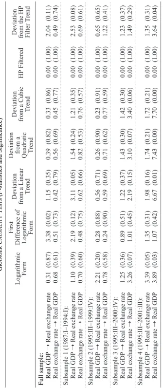
From the cross correlations presented in Table I, it is evident that there is a nega-tive correlation between the real exchange rate and output. The direction of the cau-sality seems to be from the seasonally adjusted real GDP to the real exchange rate as the magnitudes of the cross correlations are greater in lead periods than in lag peri-ods. To examine the direction of causality more precisely and control the effects of other lagged forms of these two variables, we test the relationship between the real exchange rate and output in a VAR setting and compute the relevant F-statistics to perform the causality test in Granger’s sense (hereafter, Granger causality). The Granger causality tests will indicate whether a set of lagged variables has explana-tory power on the other variables. If the computed F-statistics are significant, then we can safely claim that one variable does Granger cause the other variable. The transformations of the above cross correlation analysis are repeated in these Granger causality tests, the results of which are presented in Table II. The VAR model that is used in computing the Granger causality tests is a two endogenous variable model with four lags, a constant term, and seasonal dummies for the first three quarters.
TABLE I I G RANGER C AUSALITY T ESTS (F
-statistics and Significance)
Full sample: Real GDP
➝
Real exchange rate
Real exchange rate
➝
Real GDP
Subsample 1 (1987:I–1994:I): Real GDP
➝
Real exchange rate
Real exchange rate
➝
Real GDP
Subsample 2 (1995:III–1999:IV): Real GDP
➝
Real exchange rate
Real exchange rate
➝
Real GDP
Subsample 3 (1995:III–2000:IV): Real GDP
➝
Real exchange rate
Real exchange rate
➝
Real GDP
Subsample 4 (1995:III–2001:III): Real GDP
➝
Real exchange rate
Real exchange rate
➝
Real GDP
Deviation from the HP Filter Trend
HP Filtered
Deviation
from a Cubic
Trend
Deviation from a Quadratic Trend
Deviation from a Linear Trend First Difference of Logarithmic Form Logarithmic Form Note: p
-values are reported next to
F -statistics, in parentheses. (0.11) (0.74) (0.08) (0.61) (0.65) (0.41) (0.37) (0.29) (0.31) (0.04) 2.04 0.49 2.53 0.69 0.65 1.22 1.23 1.49 1.35 3.64 (1.00) (1.00) (1.00) (1.00) (1.00) (1.00) (1.00) (1.00) (1.00) (1.00) 0.00 0.00 0.00 0.00 0.00 0.00 0.00 0.00 0.00 0.00 (0.86) (0.77) (0.35) (0.57) (0.91) (0.59) (0.30) (0.06) (0.21) (0.00) 0.33 0.45 1.21 0.76 0.23 0.77 1.42 3.40 1.72 7.70 (0.82) (0.69) (0.24) (0.53) (0.90) (0.62) (0.30) (0.07) (0.21) (0.00) 0.39 0.56 1.54 0.82 0.26 0.71 1.43 3.10 1.74 7.43 (0.35) (0.79) (0.05) (0.66) (0.71) (0.69) (0.37) (0.15) (0.16) (0.01) 1.15 0.42 3.11 0.62 0.56 0.59 1.22 2.19 1.98 6.67 (0.02) (0.73) (0.12) (0.75) (0.88) (0.90) (0.51) (0.45) (0.31) (0.42) 3.38 0.51 2.19 0.48 0.28 0.24 0.89 1.01 1.35 1.07 (0.87) (0.61) (0.39) (0.60) (0.20) (0.58) (0.36) (0.07) (0.05) (0.03) 0.31 0.68 1.10 0.70 2.21 0.78 1.25 3.26 3.39 3.89
We first computed the relevant F-statistic values for the whole sample. The re-sults of the full sample Granger causality test state that neither of the variables is helpful in explaining the movements of the other. The null hypothesis that the real exchange rate does not Granger cause real output, and the null hypothesis that real output does not Granger cause the real exchange rate cannot be rejected even in lower levels of significance. However, for the transformation of the first difference of the logarithms of the variables, the null hypothesis that the real GDP does not Granger cause the real exchange rate is rejected at the 2 per cent level of signifi-cance. In all other transformations, there seems to be no causality between these two variables. There are at least two different ways to explain this failure of the Granger causality test in the full sample. The first is that the fifteen-year sample period is a long horizon when different characteristics of economic activity, monetary policy, and related policy tools are considered. There may be periods when the interaction between the real exchange rate and output changes. For example, for the years be-tween 1995 and 1999, the CBRT’s objective was primarily to achieve market stabil-ity. The CBRT tried to influence exchange rate movements under this constraint and for the year 2000, the exchange rate tool was used in the disinflation strategy. These counter developments may offset the possible negative effects between the vari-ables.
We re-performed the analysis for different subsamples. The 1994 devaluation was very detrimental on economic activity, and high levels of depreciation were seen in this period. Therefore, it was thought that dividing the full sample into subsamples before and after the 1994 crisis would be suitable. Thus, the first subsample is cho-sen to be the period from 1987:I, the beginning period of our full sample, to 1994:I, the last period before the crisis and devaluation of 1994. We have excluded the crisis and subsequent recession and the “V type” of the recovery period because of the ex-treme behavior of the nominal exchange rates during this period. For the post-1994 subsample, we consider three different and overlapping subsamples. Our second subsample is the period between 1995:III and 1999:IV. The last quarter of 1999 is the last quarter of the managed float regime before the implementation of the crawl-ing peg regime of the Year 2000 Disinflation Program. We also repeated the analysis to assess whether any different relationship could be detected when the period of crawling peg regime is included; hence, we extended the data span in the third sub-sample to 2000:III, the last quarter before the November 2000 banking and related liquidity crisis. In the same manner, we extended the analysis to include the crisis in February 2001 and the following recession. Neither the 2000 Disinflation Program’s crawling peg regime nor the period of the floating exchange rate regime of 2001 can be analyzed alone, due to the shortness of each time span.
The results of these subsample analyses of Granger causality tests give mixed re-sults. First of all, there is no transformation that gives a statistically significant causal relationship between the real exchange rate and output in any of the
subsam-ples considered. In the first subsample, the transformation of deviation from a linear trend and deviation from HP filtered reveal that output Granger causes the real ex-change rate at the 5 per cent and the 8 per cent levels of significance, respectively. There is no statistically significant causality relationship in either direction in the second subsample presented in Table II. In the subsample between 1995:III and 2000:IV, in three of the transformations—namely, logarithmic form of the variables, deviation from a quadratic trend, and deviation from a cubic trend—the null hy-pothesis that the real exchange rate does not Granger-cause real output is rejected at the 7 per cent level of significance. Finally, when the last subsample is considered in the majority of the transformations, it is evident that the real exchange rate Granger causes real output. In the logarithmic form, where the real exchange rate Granger causes output, output also Granger causes the real exchange rate. In the other cases, the hypothesis that output Granger causes the real exchange rate is rejected
The results of the subsample Granger causality tests are mixed but they at least give an indication and an expected result for the last subsample. In the last subsam-ple, we have considered all the periods between 1995:III and 2001:III. During this period, there are times when the real exchange rate appreciated and output increased contemporaneously or with lags, like in 2000. In 2001 as well, there is a period when the nominal and real exchange rate depreciated and recession occurred. Thus, the last subsample is sufficiently large to incorporate significant variation in the en-dogenous variables. Hence, it is large enough to deduce significant relationships be-tween variables. However, it cannot be said that the causality from the real exchange rate to real output is homogeneous in different transformations. Thus, we cannot safely conclude that the real exchange rate Granger causes real output in the last subsample.
The second possible explanation for the failure of the Granger causality tests is that we cannot remove the possible effects of exogenous variables from the consid-ered endogenous variables in this test. In other words, it is clear that other economic variables (interest rates, inflation, capital account movements, etc.) may have possi-ble effects on both variapossi-bles, and their effects may limit the usefulness of the Granger causality analysis. In the next section, the statistical properties of the data will be analyzed.
VI. STATISTICAL PROPERTIES OF THE DATA
In this section, we will analyze the stationary properties of the variables of interest, namely, the real exchange rate, inflation, and output, and a set of control variables. These control variables are government size, current account, capital account, and M1. In addition, we analyzed whether any long-term relationship among the real ex-change rate, output, and inflation exists even when some of the control variables are added into the system. Unit root tests of the variables are given in the first
subsec-tion. In the second subsection cointegration tests that explore the possible long-term relationships among these variables will be analyzed.
A. Unit Root Tests
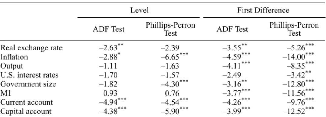
In this subsection, we analyze the unit root tests of the variables of the real ex-change rate, inflation, output, the U.S. interest rates, government size, M1, current account, and capital account. In all VAR models, we use the real exchange rate, inflation, and output. In addition, we use the variables of the U.S. interest rates, gov-ernment size (fraction of the govgov-ernment purchases item in the nominal GDP), M1, current account (ratio of the current account to the nominal GDP), and capital ac-count (ratio of the capital acac-count, excluding official reserves to the nominal GDP). All the variables enter the analysis in logarithms except variables in rates. Table III gives the unit root tests of these variables.
We use both the augmented Dickey-Fuller (ADF) test and the Phillips-Perron test for unit root tests. Both tests reveal that for output, U.S. interest rates, and M1, we cannot reject the presence of unit root, while for variables of inflation, current ac-count, and capital account we can reject the presence of unit root. In addition, while the ADF test states that the real exchange does not contain a unit root, the Phillips-Perron test states the reverse. The Phillips-Phillips-Perron test states that government size is stationary while the ADF test states the opposite. This suggests that the order of the variables of interests are mixed. In addition, for the first differences of output and M1, we can reject the presence of unit root. However, for the first difference of U.S.
TABLE III UNITROOTTESTS
Real exchange rate Inflation
Output
U.S. interest rates Government size M1 Current account Capital account **–2.63** *–2.88* –1.11 –1.70 –1.82 –0.93 ***–4.94*** ***–4.38*** –2.39 ***–6.65*** –1.63 –1.57 ***–4.30*** –0.76 ***–4.54*** ***–5.90*** **–3.55** ***–4.59*** ***–4.11*** –2.49 **–3.16** ***–3.77*** ***–4.26*** ***–3.99*** ***0–5.26*** ***–14.00*** ***0–8.35*** **0–3.42** ***–12.80*** ***–11.56*** ***0–9.76*** ***–12.52***
Level First Difference
ADF Test Phillips-PerronTest ADF Test Phillips-PerronTest
Note: In both of the tests, we use four-lag orders.
* denotes the rejection of the hypothesis that the variable does not contain unit root at the 10 per cent level of significance.
** denotes the rejection of the hypothesis that the variable does not contain unit root at the 5 per cent level of significance.
***denotes the rejection of the hypothesis that the variable does not contain unit root at the 1 per cent level of significance.
nominal interest, we can reject the presence of unit root only with the Phillips-Perron test.
B. Cointegration Tests
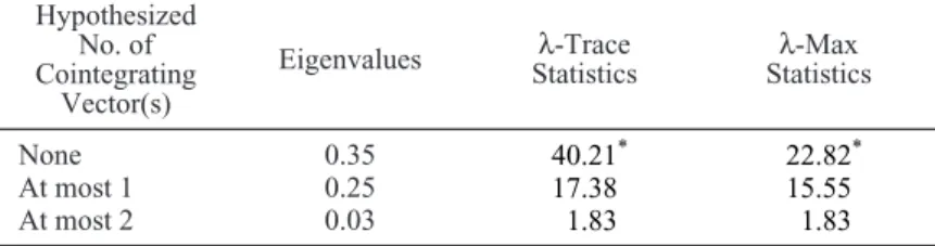
In this paper, we want to assess the effects of a real depreciation on output and inflation. To this end, we first want to analyze whether there exists any long-run re-lationship among variables of the real exchange rate, inflation, and output. Hence, we perform Johansen cointegration tests and compute the λ-trace and λ-max
eigen-value test statistics for various settings.1First of all, we want to assess a long-run
re-lationship among the variables for a minimum number of variables. Hence, the first setting explores for a long-run relationship among the real exchange rate, inflation, and output when seasonal factors and external factors, which are captured by U.S. interest rates, are kept exogenous.
As Table IV suggests, after controlling for seasonal factors and U.S. interest rates, there exists a long-run relationship among the real exchange rate, inflation, and out-put. The λ-trace and λ-max test statistics also show that there is only one cointegrat-ing vector in this settcointegrat-ing. Then, we look at whether a long-run relationship exists in other specifications, which will be elaborated on later in the text for observing the robustness of our findings. These models include M1 monetary aggregate, govern-ment size, current account, and capital account in different specifications. The find-ings of Johansen cointegration tests of these alternative settfind-ings state that there exists at least one long-run relationship in each of the alternative settings.2
As elaborated in Sims, Stock, and Watson (1990), when the variables are cointe-grated, using a VAR model in levels is consistent. Hence, we have estimated VAR models parallel to Kamin and Rogers (2000) so that the negative correlations and dynamic relation between the variables of interest can be analyzed for the core
TABLE IV
COINTEGRATIONTEST FOR THEREALEXCHANGERATE, INFLATION, ANDOUTPUT Hypothesized
No. of Cointegrating
Vector(s)
Eigenvalues Statisticsλ-Trace Statisticsλ-Max
*refers to rejection of zero cointegrating vector at 5 per cent level of sig-nificance. None At most 1 At most 2 0.35 0.25 0.03 *40.21* 17.38 01.83 *22.82* 15.55 01.83
01In order to perform Johansen cointegration tests, not all variables should be I(1) but some of the
variables might be I(0) while other variables are I(1) (see Hansen and Juselius 1995).
model and also for the alternative settings explained above for a set of robustness checks.
VII. VAR MODEL AND EMPIRICAL ANALYSIS
In this section, the core model and alternative models that our econometric analyses are based on are described first. In the second subsection, the forecast error variance decomposition analyses are explained, and the impulse responses obtained from the models are explained in the last subsection.
A. The Model
In the bivariate analysis, it was shown that there exists a negative correlation be-tween the real exchange rate and output; however, the direction of causality could not be shown due to the reasons mentioned. In the statistical analysis section, find-ings show that some of the variables have a unit root when the others do not; how-ever, it was found that a long-run relationship exists among the real exchange rate, inflation, and output. In addition, we also found that when other variables like gov-ernment size, M1, capital account, and current account are included there is a coin-tegration relation. Relying on the result of Sims, Stock, and Watson (1990), VAR models in level are derived to study the negative correlation between output and the real exchange rate more precisely and to see whether this negative relationship emerges from a spurious correlation. Another way of studying this negative rela-tionship might be the use of structural equations which are based on economic theory. However, choice of structural form is difficult and may lead to arbitrary identifying restrictions. VAR models, on the other hand, treat the variables symmetrically and provide dynamic interaction among the variables of interest. In addition, VAR mod-els have high predictive power. Hence, we use the VAR modmod-els, which also enable us to the observe impulse response functions and the forecast error variance decom-position analyses from which our findings are gathered. These VAR models also capture the sources of important external shocks.
Our core VAR model is formed by three-endogenous variables with the particular order of the real exchange rate, the inflation and the seasonally adjusted real output where U.S. nominal interest rate is used as exogenous. The order of the variables is the same as those in Kamin and Rogers.3The U.S. nominal interest rate is taken as
exogenous because Turkish economic variables like inflation, the real GDP, and the real exchange rate are not expected to have any effect on U.S. interest rates. The U.S. interest rate captures the external developments that may have significant ef-fects on the real exchange rate, inflation, and the real GDP in Turkey. In alternative models, we add other variables like government size, balance of payments items,
and M1 monetary aggregate. Given that we use quarterly data, our VAR models have four lags and use constant terms and seasonal dummies for the first three quar-ters.4In the first alternative model, we include government size as an additional
vari-able in the core model setting. Government size is included in the core model because government purchases and public sector prices are influential in the GDP and inflation, and it may also have an effect on the level of the real exchange. In the second alternative model, we augment the M1 monetary aggregate variable to the core model. M1 is included to capture the monetary channel to the formation of the real exchange rate, inflation, and output. The third alternative model uses the added variable of the current account. As a balance of payments item, the current account is expected to have effects on the real exchange rate. Moreover, the current account affects the GDP directly and it influences inflation and output via indirect channels. The size of capital flows affects the nominal exchange rate directly by changing the supply and demand in the exchange rate market, and thus the real exchange rate. It also has indirect effects on inflation and output. Thus, the fourth alternative model incorporates the capital account variable in the core model. In the last alternative model, the exogenous variable of U.S. interest rate is excluded, and the capital ac-count and government size are included with the variables of the real exchange rate, inflation, and output because we want to see the dynamic interrelationship among the domestic variables in a setting that assumes the weaknesses of international links.
B. Forecast Error Variance Decompositions
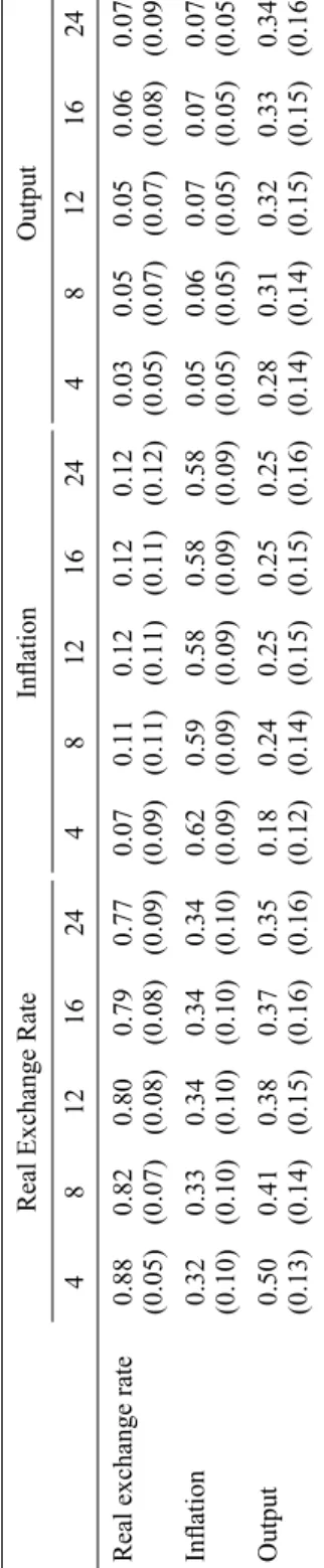
In Table V, we present the forecast error variance decompositions of the variables used in the core VAR model. These are fractions of the forecast error variances of the variables attributed to their own innovations or the innovations of the other vari-ables. The forecast error variances of the variables will give information about shocks that have explanatory power to forecast variables. After obtaining the model estimates, in order to calculate the standard errors, we have used the bootstrap pro-cedure, and the number of bootstrap draws was chosen to be three thousand.
We have reported the forecast error variance decompositions at the 4, 8, 12, 16, and 24 periods. The variables in the rows are the ones whose forecast error variance decompositions are in question, and the variables in the columns are those whose innovations constitute the fraction of the variables in the column. For example, 0.88 is the fraction of the forecast error variance in the real exchange rate that is attributed to its own innovation at the four-quarter forecast horizon, and the associated stan-dard error for this fraction is 0.05. We have reported the forecast error variances of the real exchange rate, inflation, and the output.
04We have tried shorter lag lengths and the findings from these models are parallel to our core model
TABLE V F ORECAST E RROR V ARIANCE D ECOMPOSITION OF V ARIABLES IN THE C ORE M ODEL
Real exchange rate Inflation Output
Output
Inflation
Real Exchange Rate
Note: Standard errors are reported in parentheses under fractions of forecast errors estimated.
24 0.07 (0.09) 0.07 (0.05) 0.34 (0.16) 16 0.06 (0.08) 0.07 (0.05) 0.33 (0.15) 12 0.05 (0.07) 0.07 (0.05) 0.32 (0.15) 8 0.05 (0.07) 0.06 (0.05) 0.31 (0.14) 4 0.03 (0.05) 0.05 (0.05) 0.28 (0.14) 24 0.12 (0.12) 0.58 (0.09) 0.25 (0.16) 16 0.12 (0.11) 0.58 (0.09) 0.25 (0.15) 12 0.12 (0.11) 0.58 (0.09) 0.25 (0.15) 8 0.11 (0.11) 0.59 (0.09) 0.24 (0.14) 4 0.07 (0.09) 0.62 (0.09) 0.18 (0.12) 24 0.77 (0.09) 0.34 (0.10) 0.35 (0.16) 16 0.79 (0.08) 0.34 (0.10) 0.37 (0.16) 12 0.80 (0.08) 0.34 (0.10) 0.38 (0.15) 8 0.82 (0.07) 0.33 (0.10) 0.41 (0.14) 4 0.88 (0.05) 0.32 (0.10) 0.50 (0.13)
Table V shows that the most important source of variation in the real exchange rate forecast error is its own innovations, which account for 77–88 per cent of the variance of its forecast. As seen in Table V, innovations in inflation account for 7–12 per cent and innovations in output account for only 3–7 per cent of the forecast error variance of the real exchange rate. These findings show that innovations in the other variables have little power to explain the variation in the real exchange rate; thus, it can be argued that the real exchange rate is exogenous. These findings may also sug-gest that the CBRT might be using this variable as a policy tool in the sample period. The findings are statistically significant for the real exchange rate innovations for all the periods.5
Similar to the real exchange rate, inflation’s own innovations account for the highest fraction of its forecast error variance. It accounts for 58–62 per cent of the forecast error variance. The second important source of forecast error variance of inflation is the innovations in the real exchange rate. It explains 32–34 per cent of the forecast error variance of inflation. These show that real exchange rate move-ments are important in the variability of the forecast error of inflation. The weakest source of the forecast error variance of inflation is output. It accounts for only 5–7 per cent of the forecast error variance of inflation. Observations for inflation and real exchange rate innovations are statistically significant throughout the twenty-four-quarter forecast horizon in explaining the forecast error variance of inflation.
There exists an interesting case for forecast error variance of output. In contrast to the real exchange rate and inflation, the innovations of output are not the most im-portant source in explaining the forecast error variance of output. Innovations in the real exchange rate account for 35–50 per cent and innovations in output explain 28– 34 per cent of the forecast error variance of output. These two are the most impor-tant factors in explaining the variance of output. Innovations in inflation are the third most important source of the forecast error variance of output and they explain 18–25 per cent of the forecast error variance of output. All findings, except those for innovations in inflation for the fourth and twenty-fourth forecast period, are statisti-cally significant.
The findings in the above forecast error variance decompositions reveal that real exchange rate movements influence the level of the real GDP and inflation but are not influenced by any endogenous variable in the model. Likewise, inflationary shocks explain the movements in output, but shocks to output do not explain any of the variables in the system.
After obtaining the forecast error variances of the endogenous variables in the core model, we have computed the forecast error variances of the variables in the alternative models to assess the robustness of the results that have been arrived at in the forecast error variance decomposition analysis of the core model. We have
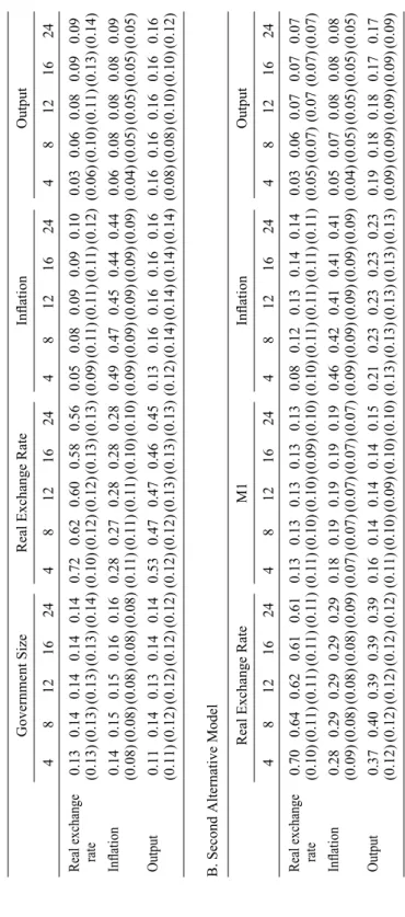
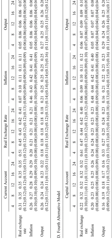
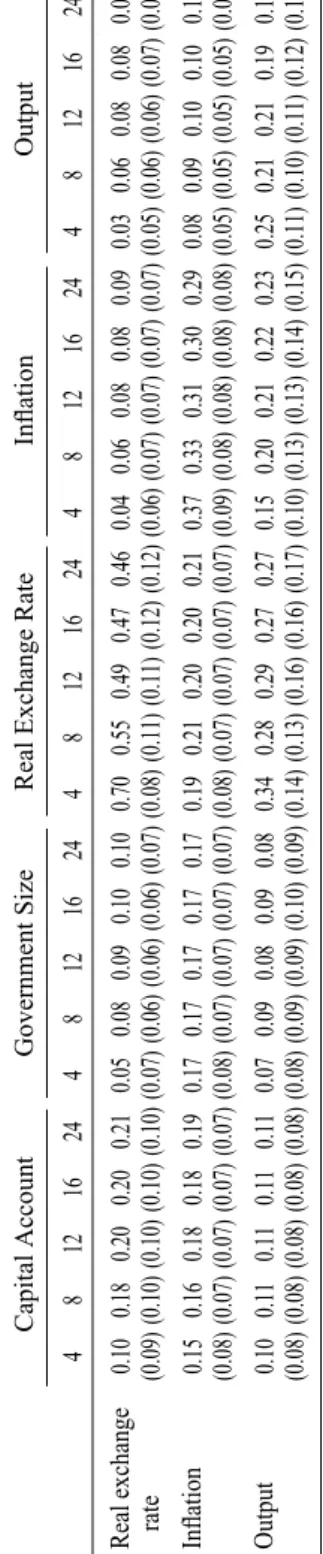
veloped five other VAR models with four lags and a variable is added in each of the models. We include government size as an additional variable in the first alternative model with the particular order of government size, the real exchange rate, inflation, and output. In the second alternative model, we augment the M1 monetary aggre-gate variable and use the particular order of the real exchange rate, M1, inflation, and output. The third alternative model uses the added variable of the current ac-count with the particular order of current acac-count, the real exchange rate, inflation, and output. The fourth alternative model incorporates the capital account variable and the particular order of the model is the capital account, the real exchange rate, inflation, and output. All of these models use the U.S. interest rate as exogenous, while in the last alternative model, the U.S. interest rate is excluded and the capital account and government size are included with the variables of interest. We want to see the dynamic interrelationship between the domestic variables in a setting that assumes the weaknesses of international links. The particular order of the last alter-native model is capital account, government size, the real exchange rate, inflation, and output. In Table VI, as in Table V, the variables in the columns are the variables whose innovations constitute the forecast error variance, and the variables in the rows are the variables whose forecast error variance is in question, namely, the real exchange rate, inflation, and output. The variables in the columns are presented cor-respondingly to their order in the VAR models.
From the forecast error variance decomposition analysis of the core model, we have arrived at the conclusion that the movements of output and inflation do not influence real exchange movements. From the alternative models, it is evident that the balance of payments items—the current account and the capital account—are helpful in explaining the forecast error variance of the real exchange rate. From the alternative models, this may suggest that the main balance of payments items are ef-fective in explaining the forecast error variance of the real exchange rate. This may mean that the CBRT aligned its exchange rate policy by observing these variables in the sample period that we consider. However, other endogenous variables of inter-est—inflation and output—are not useful in explaining the forecast error variance of the real exchange rate. Innovations in inflation account for 4–14 per cent and in-novations in output 3–10 per cent of the forecast error variance of the real exchange in the alternative models. Thus, parallel to the conclusion that was drawn from the forecast error variances of the core model, inflation and output do not influence the real exchange rate.
The innovations in the real exchange rate are helpful in the forecast error variance of inflation in the core model. As seen in Table VI, innovations in the real exchange rate are helpful in explaining the forecast error variance of inflation in all of the al-ternative models. Innovations in the real exchange rate account for 19–28 per cent of the forecast error variance of inflation in the alternative models. However, from the alternative models that include the balance of payments items, we reach the
conclu-TABLE V I F ORECAST E RROR V ARIANCE D ECOMPOSITIONS OF A LTERNATIVE M ODELS
Real exchange rate Inflation Output
8 0.14 (0.13) 0.15 (0.08) 0.14 (0.12) 12 0.14 (0.13) 0.15 (0.08) 0.13 (0.12) 16 0.14 (0.13) 0.16 (0.08) 0.14 (0.12) 24 0.14 (0.14) 0.16 (0.08) 0.14 (0.12) 4 0.72 (0.10) 0.28 (0.11) 0.53 (0.12) 8 0.62 (0.12) 0.27 (0.11) 0.47 (0.12) 12 0.60 (0.12) 0.28 (0.11) 0.47 (0.13) 16 0.58 (0.13) 0.28 (0.10) 0.46 (0.13) 24 0.56 (0.13) 0.28 (0.10) 0.45 (0.13) 4 0.05 (0.09) 0.49 (0.09) 0.13 (0.12) 8 0.08 (0.11) 0.47 (0.09) 0.16 (0.14) 12 0.09 (0.11) 0.45 (0.09) 0.16 (0.14) 16 0.09 (0.11) 0.44 (0.09) 0.16 (0.14) 24 0.10 (0.12) 0.44 (0.09) 0.16 (0.14) 4 0.03 (0.06) 0.06 (0.04) 0.16 (0.08) 8 0.06 (0.10) 0.08 (0.05) 0.16 (0.08) 12 0.08 (0.11) 0.08 (0.05) 0.16 (0.10) 16 0.09 (0.13) 0.08 (0.05) 0.16 (0.10) 24 0.09 (0.14) 0.09 (0.05) 0.16 (0.12) 4 0.13 (0.13) 0.14 (0.08) 0.11 (0.11)
A. First Alternative Model
Government Size
Real Exchange Rate
Inflation
Output
Real exchange rate Inflation Output
8 0.64 (0.11) 0.29 (0.08) 0.40 (0.12) 12 0.62 (0.11) 0.29 (0.08) 0.39 (0.12) 16 0.61 (0.11) 0.29 (0.08) 0.39 (0.12) 24 0.61 (0.11) 0.29 (0.09) 0.39 (0.12) 4 0.13 (0.11) 0.18 (0.07) 0.16 (0.11) 8 0.13 (0.10) 0.19 (0.07) 0.14 (0.10) 12 0.13 (0.10) 0.19 (0.07) 0.14 (0.09) 16 0.13 (0.09) 0.19 (0.07) 0.14 (0.10) 24 0.13 (0.10) 0.19 (0.07) 0.15 (0.10) 4 0.08 (0.10) 0.46 (0.09) 0.21 (0.13) 8 0.12 (0.11) 0.42 (0.09) 0.23 (0.13) 12 0.13 (0.11) 0.41 (0.09) 0.23 (0.13) 16 0.14 (0.11) 0.41 (0.09) 0.23 (0.13) 24 0.14 (0.11) 0.41 (0.09) 0.23 (0.13) 4 0.03 (0.05) 0.05 (0.04) 0.19 (0.09) 8 0.06 (0.07) 0.07 (0.05) 0.18 (0.09) 12 0.07 (0.07 0.08 (0.05) 0.18 (0.09) 16 0.07 (0.07) 0.08 (0.05) 0.17 (0.09) 24 0.07 (0.07) 0.08 (0.05) 0.17 (0.09) 4 0.70 (0.10) 0.28 (0.09) 0.37 (0.12)
B. Second Alternative Model
Real Exchange Rate
M1
Inflation
Real exchange rate Inflation Output 8 0.35 (0.12) 0.27 (0.10) 0.24 (0.11) 12 0.35 (0.12) 0.28 (0.10) 0.24 (0.11) 16 0.35 (0.13) 0.29 (0.09) 0.23 (0.11) 24 0.35 (0.13) 0.29 (0.10) 0.22 (0.11) 4 0.51 (0.12) 0.20 (0.08) 0.18 (0.11) 8 0.45 (0.12) 0.21 (0.08) 0.18 (0.11) 12 0.43 (0.12) 0.21 (0.08) 0.18 (0.12) 16 0.42 (0.12) 0.21 (0.08) 0.18 (0.12) 24 0.41 (0.13) 0.21 (0.08) 0.18 (0.13) 4 0.07 (0.09) 0.46 (0.10) 0.21 (0.14) 8 0.10 (0.09) 0.43 (0.09) 0.25 (0.14) 12 0.11 (0.09) 0.42 (0.09) 0.25 (0.14) 16 0.11 (0.09) 0.41 (0.09) 0.25 (0.15) 24 0.11 (0.09) 0.41 (0.09) 0.25 (0.16) 4 0.05 (0.06) 0.05 (0.04) 0.27 (0.11) 8 0.06 (0.06) 0.06 (0.04) 0.25 (0.11) 12 0.06 (0.06) 0.06 (0.04) 0.25 (0.11) 16 0.06 (0.06) 0.06 (0.04) 0.26 (0.12) 24 0.07 (0.06) 0.06 (0.04) 0.26 (0.12) 4 0.31 (0.12) 0.26 (0.10) 0.26 (0.12)
C. Third Alternative Model
Current Account
Real Exchange Rate
Inflation
Output
Real exchange rate Inflation Output
8 0.32 (0.11) 0.23 (0.08) 0.19 (0.12) 12 0.32 (0.11) 0.25 (0.08) 0.18 (0.11) 16 0.32 (0.11) 0.25 (0.08) 0.17 (0.12) 24 0.32 (0.11) 0.26 (0.09) 0.16 (0.12) 4 0.61 (0.10) 0.24 (0.08) 0.33 (0.13) 8 0.47 (0.12) 0.24 (0.08) 0.27 (0.13) 12 0.44 (0.12) 0.23 (0.08) 0.25 (0.15) 16 0.42 (0.12) 0.23 (0.08) 0.24 (0.16) 24 0.40 (0.12) 0.23 (0.08) 0.23 (0.18) 4 0.06 (0.08) 0.48 (0.09) 0.16 (0.13) 8 0.09 (0.08) 0.44 (0.08) 0.21 (0.14) 12 0.10 (0.09) 0.42 (0.08) 0.22 (0.15) 16 0.11 (0.09) 0.41 (0.08) 0.23 (0.15) 24 0.12 (0.10) 0.40 (0.08) 0.23 (0.16) 4 0.06 (0.07) 0.05 (0.04) 0.29 (0.11) 8 0.07 (0.06) 0.07 (0.04) 0.24 (0.13) 12 0.09 (0.07) 0.07 (0.04) 0.26 (0.14) 16 0.09 (0.08) 0.07 (0.04) 0.25 (0.16) 24 0.10 (0.09) 0.08 (0.04) 0.26 (0.17) 4 0.22 (0.10) 0.20 (0.08) 0.16 (0.09)
D. Fourth Alternative Model
Capital Account
Real Exchange Rate
Inflation
Output
TABLE V
TABLE V
I (Continued)
Real exchange rate Inflation Output
8 0.18 (0.10) 0.16 (0.07) 0.11 (0.08) 12 0.20 (0.10) 0.18 (0.07) 0.11 (0.08) 16 0.20 (0.10) 0.18 (0.07) 0.11 (0.08) 24 0.21 (0.10) 0.19 (0.07) 0.11 (0.08) 4 0.05 (0.07) 0.17 (0.08) 0.07 (0.08) 8 0.08 (0.06) 0.17 (0.07) 0.09 (0.09) 12 0.09 (0.06) 0.17 (0.07) 0.08 (0.09) 16 0.10 (0.06) 0.17 (0.07) 0.09 (0.10) 24 0.10 (0.07) 0.17 (0.07) 0.08 (0.09) 4 0.70 (0.08) 0.19 (0.08) 0.34 (0.14) 8 0.55 (0.11) 0.21 (0.07) 0.28 (0.13) 12 0.49 (0.11) 0.20 (0.07) 0.29 (0.16) 16 0.47 (0.12) 0.20 (0.07) 0.27 (0.16) 24 0.46 (0.12) 0.21 (0.07) 0.27 (0.17) 4 0.04 (0.06) 0.37 (0.09) 0.15 (0.10) 8 0.06 (0.07) 0.33 (0.08) 0.20 (0.13) 12 0.08 (0.07) 0.31 (0.08) 0.21 (0.13) 16 0.08 (0.07) 0.30 (0.08) 0.22 (0.14) 24 0.09 (0.07) 0.29 (0.08) 0.23 (0.15) 4 0.03 (0.05) 0.08 (0.05) 0.25 (0.11) 8 0.06 (0.06) 0.09 (0.05) 0.21 (0.10) 12 0.08 (0.06) 0.10 (0.05) 0.21 (0.11) 16 0.08 (0.07) 0.10 (0.05) 0.19 (0.12) 24 0.08 (0.07) 0.11 (0.05) 0.19 (0.13) 4 0.10 (0.09) 0.15 (0.08) 0.10 (0.08)
E. Fifth Alternative Model
Capital Account
Government Size
Real Exchange Rate
Inflation
Output