Efficient computation of surface fields excited on an electrically large circular cylinder with an impedance boundary condition

(1)

EFFICIENT COMPUTATION OF SURFACE

FIELDS EXCITED ON AN ELECTRICALLY

LARGE CIRCULAR CYLINDER WITH AN

IMPEDANCE BOUNDARY CONDITION

a thesis

submitted to the department of electrical and

electronics engineering

and the institute of engineering and science

of bilkent university

in partial fulfillment of the requirements

for the degree of

master of science

By

Burak Ali¸san

(2)

I certify that I have read this thesis and that in my opinion it is fully adequate, in scope and in quality, as a thesis for the degree of Master of Science.

Prof. Dr. Ayhan Altınta¸s (Advisor)

Asst. Prof. Dr. Vakur B. Ert¨urk (Co-advisor)

Prof. Dr. Orhan Arıkan

Prof. Dr. G¨ulbin Dural

Asst. Prof. Dr. Lale Alatan

Approved for the Institute of Engineering and Science:

Prof. Dr. Mehmet Baray Director of the Institute

(3)

ABSTRACT

EFFICIENT COMPUTATION OF SURFACE FIELDS

EXCITED ON AN ELECTRICALLY LARGE

CIRCULAR CYLINDER WITH AN IMPEDANCE

BOUNDARY CONDITION

Burak Ali¸san

M.S. in Electrical and Electronics Engineering Supervisor: Prof. Dr. Ayhan Altınta¸s

July, 2006

An efficient computation technique is developed for the surface fields excited on an electrically large circular cylinder with an impedance boundary condition (IBC). The study of these surface fields is of practical interest due to its appli-cations in the design and analysis of conformal antennas. Furthermore, it acts as a canonical problem useful toward the development of asymptotic solutions valid for arbitrary smooth convex thin material coated/partially material coated surfaces.

In this thesis, an alternative numerical approach is presented for the evalua-tion of the Fock type integrals which exist in the Uniform Geometrical Theory of Diffraction (UTD) based asymptotic solution for the non-paraxial surface fields excited by a magnetic or an electric source located on the surface of an elec-trically large circular cylinder with an IBC. This alternative approach is based on performing a numerical integration of the Fock type integrals on a deformed path on which the integrands are non-oscillatory and rapidly decaying. Compar-ison of this approach with the previously developed study presented by Tokg¨oz (PhD thesis, 2002), which is based on invoking the Cauchy’s residue theorem by finding the pole singularities numerically, reveals that the alternative approach is considerably more efficient. Since paraxial solution is a closed-form solution and very efficient in terms of computational time, there is no need for an alternative approach for the evaluation of the paraxial surface fields.

Keywords: Surface fields, Impedance cylinder, UTD based Green’s functions, Fock type integrals.

(4)

¨

OZET

EMPEDANS SINIR KOS

¸ULLARI OLAN ELEKTR˙IKSEL

OLARAK B ¨

UY ¨

UK B˙IR C

¸ EMBERSEL S˙IL˙IND˙IR

¨

UZER˙INDEK˙I Y ¨

UZEY DALGALARININ VER˙IML˙I

S

¸EK˙ILDE HESAPLANMASI

Burak Ali¸san

Elektrik ve Elektronik Mühendisli˘gi, Yüksek Lisans Tez Yöneticisi: Ayhan Altınta¸s

Temmuz, 2006

Empedans sınır ko¸sulları olan elektriksel olarak b¨uy¨uk bir ¸cembersel silindir ¨

uzerinde olu¸sturulan yüzey dalgaları i¸cin verimli bir hesaplama tekni˘gi geli¸stirilmi¸stir. Bu yüzey dalgaları üzerinde yapılan ¸cal¸sma konformal antenlerin tasarım ve analiz uygulamalarından dolayı önemlidir. Ayrıca, tamamen veya kısmen ince materyal kaplı dı¸sbükey yüzeyler i¸cin ge¸cerli asimptotik ¸cözümlerin geli¸stirilmesinde yararlı olacak kanonik bir problem gibi davranır.

Bu tezde, empedans sınır ko¸sulları olan elektriksel olarak büyük bir ¸cembersel silindir üzerine yerle¸stirilmi¸s bir manyetik veya elektrik kayna˘gı tarafından olu¸sturulan eksensel olmayan yüzey dalgaları i¸cin ge¸cerli olan UTD’ye dayalı asimptotik ¸cözümlerde bulunan Fock tipi integrallerin hesaplanması i¸cin al-ternatif bir sayısal yakla¸sım sunulmu¸stur. Bu alternatif yakla¸sım, Fock tipi integrallerin salınımsız oldu˘gu ve hızla azaldı˘gı bi¸cimi bozulmu¸s bir yol ¨

uzerindeki sayısal integrasyonununa dayandırılmı¸stır. Bu yakla¸sımın daha önce Tokgöz (Doktora tezi, 2002) tarafından geli¸stirilmi¸s kutup tekilliklerinin sayısal olarak bulunarak Cauchy residue teoreminin uygulanmasına dayandırılmı¸s yakla¸sımla kar¸sıla¸stırılması alternatif yakla¸sımın ¸cok daha verimli oldu˘gunu or-taya ¸cıkarmı¸stır. Eksensel ¸cözümün bir kapalı form ¸cözüm olması ve hesaplama zamanı bakımından ¸cok verimli olmasından dolayı, eksensel yüzey dalgalarının hesaplanmasında bir alternatif yakla¸sıma ihtiya¸c yoktur.

Anahtar sözcükler: Yüzey dalgaları, Empedans silindiri, UTD’ye dayalı Green fonksiyonu, Fock tipi integraller.

(5)

(6)

Acknowledgement

I would like to express my gratitude to my advisors Prof. Dr. Ayhan Altınta¸s and Asst. Prof. Dr. Vakur B. Ert¨urk for their instructive comments and continuing support in the supervision of the thesis.

I would like to express my special thanks and gratitude to Prof. Dr. Orhan Arıkan, Prof. Dr. G¨ulbin Dural and Asst. Prof. Dr. Lale Alatan for showing keen interest to the subject matter and accepting to read and review the thesis.

Finally I would like to thank Aselsan Inc. for letting me to involve in this thesis study and my family for their support.

(7)

List of Figures

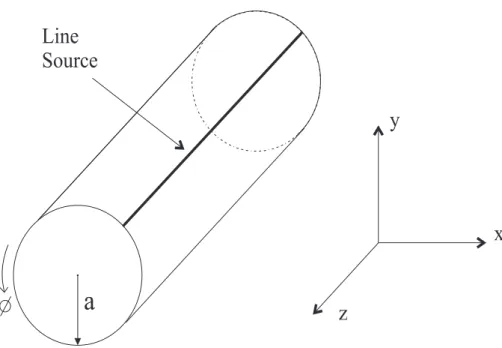
2.1 Line source on a circular cylinder with a radius a . . . 6 2.2 Geometry of a circular cylinder with a radius a . . . 8

3.1 Definition of uniformly spaced points, qt. . . 19

3.2 Paths of integration (a) Original path. (b) Deformed path 1. (c) Deformed path 2, used when the dominant pole is very close to the integration path (like an Elliott mode). . . 23 3.3 (a) Real and (b) Imaginary parts of integrand of a typical Fock

type integral (in this case integrand of Υ1) along the original and

deformed paths. . . 25

4.1 Comparison of the magnitude (in dB) of the Green’s function (2-D case) versus azimuthal angle, φ, obtained by the the numerical approaches for ka = 5. . . 30 4.2 Comparison of the magnitude (in dB) and phase of the Gm

zz

ver-sus separation, s, obtained by the eigenfunction solution and the numerical approaches for f = 7GHz, a = 5λ, α = 45◦ _{and Λ = 0.1. 32}

4.3 Comparison of the magnitude (in dB) and phase of the Gm zφ

(10)

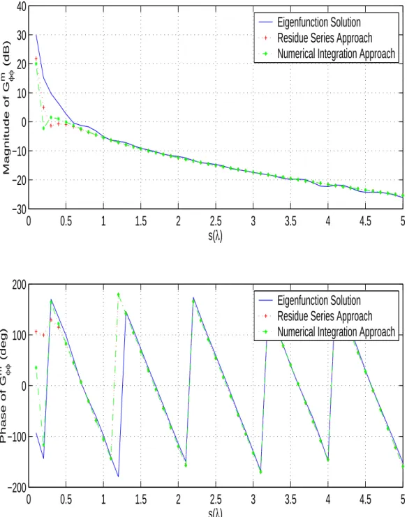
4.4 Comparison of the magnitude (in dB) and phase of the Gm φφ

4.5 Comparison of the magnitude (in dB) and phase of the Gezz

4.6 Comparison of the magnitude (in dB) and phase of the Ge zφ

4.7 Comparison of the magnitude (in dB) and phase of the Ge φφ

4.8 Comparison of the magnitude (in dB) and phase of the Gm

zz versus

separation, s, obtained by the eigenfunction solution, the UTD based and paraxial solutions for f = 7GHz, a = 5λ, α = 80◦ _and

Λ = 0.1. . . 39 4.9 Comparison of the magnitude (in dB) and phase of the Gm

zz versus

azimuthal angle, φd, obtained by the eigenfunction solution and

the UTD based (evaluated by the numerical integration approach) and paraxial solutions for f = 7GHz, a = 5λ, zd= 3λ and Λ = 0.1. 40

zφversus

φφversus

(11)

C.1 Integration paths, C+ and C−, and pole singularities on the

com-plex ν plane. . . 56

(12)

Chapter 1 Introduction

Many military and commercial applications (e.g., missiles, mobile base stations, transreceivers of Multi Input Multi Output (MIMO) systems which might be mounted on curved host platforms, etc.) have stringent aerodynamic constraints that require the use of antennas that conform to their host platforms. This ne-cessitates the development of efficient and accurate design and analysis tools for this class of antennas. Therefore, surface fields, created by a current distribu-tion on the surface of a thin material coated (lossy or lossless) perfect electric conducting (PEC) circular cylinder, have been studied extensively using an im-pedance boundary condition (IBC). Analysis of slot/aperture antennas as well as antennas on partially coated host platforms are typical applications which re-quire the fast and accurate evaluation of these surface fields. Furthermore, the study of these surface fields acts as a canonical problem useful toward the devel-opment of asymptotic solutions valid for arbitrary smooth convex thin material coated/partially material coated surfaces [1], [2].

High frequency based asymptotic solutions for the surface fields on a source excited PEC convex surface have been investigated previously. Approximate expressions were obtained for the magnetic field induced by slots on electrically large conducting circular cylinder [3]. Later, improved Geometrical Theory of Diffraction (GTD) and Uniform Geometrical Theory of Diffraction (UTD) based representations were presented for the surface fields due to a slot on a PEC

(13)

cylinder [4]. A simple approximate expression for the surface magnetic field due to a magnetic dipole on a conducting circular cylinder was developed in [5]. The surface field solution obtained in [5] contains an additional term taken from [6] because of the need to obtain an accurate solution in the paraxial (nearly axial) region of the cylinder. Furthermore, an approximate asymptotic solution was presented for the electromagnetic fields which are induced on an electrically large perfectly conducting smooth convex surface by an infinitesimal magnetic or electric current moment on the same surface [7]. In [8], the accuracy of the existing approximate asymptotic solutions for the surface field due to a magnetic dipole on a large conducting cylinder was tested by comparing them with the exact modal solution. Based on this comparison, a new approximate solution with improved accuracy for the surface field due to a magnetic point source on a cylinder was presented in [9].

However, the study of surface fields created by a current distribution on the surface of an impedance circular cylinder, which can also model a thin (lossy/lossless) material coated PEC case [10], is still a challenging problem. Recently, several high frequency based asymptotic solutions for the surface fields on a source excited circular cylinder with an IBC have been presented valid away from the paraxial region, and within the paraxial region. High frequency based solution for a surface field excited by a magnetic line source on an impedance cylinder has been presented in [11]. Later, a high frequency asymptotic solution has been introduced for the vector potentials for a point source on an anisotropic impedance cylinder [12]. In [13], an approximate asymptotic solution based on the Uniform Geometrical Theory of Diffraction (UTD) has been proposed for the magnetic fields excited at a point by an infinitesimal magnetic current moment located at another point, both on the surface of an electrically large circular cylin-der with a finite surface impedance. Afterwards, approximate solutions have been developed for the surface magnetic field on a magnetic current excited circular cylinder with an IBC in [14]. Recently, an alternative approximate asymptotic closed-form solution has been proposed for the accurate representation of the tan-gential surface magnetic field within the paraxial region of a tantan-gential magnetic current excited circular cylinder with an IBC in [15].

(14)

Among these aforementioned works related to impedance circular cylinders, the UTD based asymptotic solution for a three dimensional geometry (circular cylinder with an IBC) [12]-[14] (valid away from the paraxial region) involves some Fock type integrals and their derivatives which have to be evaluated numerically. However, special care is required in the computation of these integrals since the efficiency and accuracy of the overall solution strongly depends on the numerical evaluation of these integrals. In [14] (and in [12]-[13]), these Fock type integrals have been evaluated by invoking the Cauchy’s residue theorem, which requires finding the corresponding pole singularities numerically. It is claimed that the residue contributions coming from the first 20 poles yield sufficient accuracy.

Keeping this issue in mind, in this thesis, an alternative numerical approach is proposed for the evaluation of the Fock type integrals (and their derivatives) which is based on performing a numerical integration along a deformed path. On this path, the Fock type integrals exhibit a non oscillatory and rapidly decaying nature. Hence, using a simple Gaussian quadrature algorithm is enough to obtain very accurate results efficiently. Consequently, this alternative approach is easier to implement and requires less computational time compared to the approach presented in [14]. It should be noted that, the concept of performing a numerical integration on similar deformed integration paths has been previously used for the evaluation of surface fields of source excited electrically large dielectric coated circular cylinders in [16]-[19], and accurate results have been obtained. Moreover, the UTD based surface fields due to a tangential electric current source, which are valid away from the paraxial region, are also derived using an IBC, and evaluated both performing an integration along the aforementioned deformed path and invoking the Cauchy’s residue theorem (similar to [14]), whereas in [14] only the magnetic source case was considered.

Besides, the approximate closed-form solution given for the tangential surface magnetic field within the paraxial region of a tangential magnetic current excited circular cylinder with an IBC in [14] and [15] is briefly reviewed. In this solution, Green’s function representations are written in terms of spectral double integrals involving Hankel function. The integrals are evaluated approximately using the large argument representation of the Hankel function. Since it is a closed-form

(15)

solution, it is very efficient in terms of the computational time. Thus, UTD based solution (valid in the non-paraxial region), evaluated with numerical integration approach, and closed-form paraxial solution form a complete and efficient solution for the Green’s function representations pertaining the surface magnetic field on an electrically large circular cylinder with an IBC.

The organization of this thesis is as follows: In Section II, the UTD based asymptotic solutions for the surface fields excited by both a magnetic and an electric line source (2-D case), as well as both a magnetic and an electric point source (3-D case) located on the surface of an electrically large impedance cylinder are given. The numerical evaluation of these surface fields are discussed in Section III, which presents a review of the approach presented in [14], and a detailed description of the alternative approach, namely the numerical integration along a deformed integration path, and closed-form solution given for surface fields in paraxial region. In Section IV, several numerical results for the surface fields for both 2-D and 3-D cases are obtained using the two aforementioned approaches. An ejwt time dependence is assumed and suppressed throughout this thesis.

(16)

Chapter 2 An Asymptotic Solution for the

Surface Fields Excited on a

Circular Cylinder with an IBC

2.1 Two-Dimensional Case

In this section, an asymptotic solution for the magnetic field due to a magnetic line source excitation, given in [11], is briefly reviewed, and an asymptotic solution for the electric field due to an electric source excitation is introduced. Consider a circular cylinder with an IBC as shown in Fig. 2.1. The cylinder has a radius a, a uniform surface impedance Zs, and is oriented along the z axis.

2.1.1 Solution to the T E

z

Problem

An asymptotic solution for the magnetic field excited by a magnetic line source ~

M = ˆzM0 is presented. Magnetic field excited by ~M has only a ˆz component,

and satisfies the inhomogeneous scalar wave equation (∇2+ k2)Hz =

jk Z0

(17)

a

Line

Source

y

z

x

Figure 2.1: Line source on a circular cylinder with a radius a

where k is the free space wave number, and Z0 is the intrinsic impedance of the

free space. The impedance boundary condition at the surface of the cylinder (ρ = a) is given as

∂Hz

∂ρ − jkΛHz = 0 (2.2)

where Λ = Zs/Z0 is the normalized surface impedance. The solution to the

surface magnetic field has the form

Hz(ρ = a, φ) = −

jk Z0

Gm (2.3)

where Gm _{is the summation of all ray encirclements, which are propagating in}

the positive and negative φ directions around the cylinder. In [11], for the cal-culation of Gm _{only the two dominant surface ray contributions are taken into}

consideration, and Gm _{is expressed as}

Gm _∼ −j 2 H (2) 0 (kt1)ν(ξ1, q) − j 2H (2) 0 (kt2)ν(ξ2, q) (2.4) where ξ1,2 = mφ1,2 ; t1,2 = aφ1,2 (2.5) with m = (ka/2)1/3; φ1 = φ ; φ2 = 2π − φ (2.6)

(18)

q = −jmΛ (2.7) and ν(ξ, q) = 1 2e jπ/4r ξ π Z ∞ −∞ e−jξτ Rw − q dτ (2.8)

with Rw = W2′(τ )/W2(τ ), W2(τ ) is a Fock-type Airy function, W2′(τ ) is its

deriv-ative with respect to τ .

2.1.2 Solution to the T M

z

Problem

An asymptotic solution for the electric field excited by an electric line source ~

J = ˆzJ0 is presented. The electric field excited by ~J has only a ˆz component,

and satisfies the inhomogeneous scalar wave equation given by

(∇2+ k2)Ez = jkZ0J0. (2.9)

The impedance boundary condition at the surface of the cylinder (ρ = a) is ∂Ez

∂ρ − jkΛ

−1_E

z = 0 (2.10)

where Λ = Zs/Z0 is the normalized surface impedance. The solution to the

surface electric field has the form

Ez(ρ = a, φ) = −jkZ0Ge (2.11)

where Ge _{can be expressed as}

Ge _∼ −j 2 H (2) 0 (kt1)ν(ξ1, q) − j 2H (2) 0 (kt2)ν(ξ2, q) (2.12)

in which q = −jmΛ−1_{, and Fock type integral ν(ξ, q) is the same function given}

by (2.8).

As expected, the ˆz component of the electric field, Ez, obtained for the electric

line source excitation is the dual of the ˆz component of the magnetic field, Hz,

(19)

Z

s primary ray path

x

z

y

source point field point

a

s

φ

α

Figure 2.2: Geometry of a circular cylinder with a radius a

2.2 Three-Dimensional Case

Consider an electrically large circular cylinder with an IBC as shown in Fig. 2.2. The cylinder has a radius a, a uniform surface impedance Zs, and is assumed to

be infinitely long along its axial direction.

2.2.1 Solution to the Surface Fields in the Non-paraxial

Region (UTD Based Solution)

An asymptotic solution for the surface fields excited by a magnetic or an electric source located on the surface of a circular cylinder is derived using Airy function approximation of Hankel function.

(20)

A. Magnetic Source Excitation

For such a cylinder, ˆz components of the electric and magnetic fields due to a tangential magnetic source

~

Pm = Pmzz + Pˆ mφφˆ (2.13)

located on the surface is expressed in [14] as

Ez = 1 4π2_a Z ∞ −∞ dkze−jkzzd ∞ X n=−∞ ejnφd Dc [nkz k2 ρa P_mz + (1 + jΛ−1k kρ Rn)Pmφ] Hn(2)(kρρ) Hn(2)(kρa) (2.14) Hz = − 1 4π2_aZ s Z ∞ −∞ dkze−jkzzd ∞ X n=−∞ ejnφd Dc [(1 + jΛk kρ Rn)Pmz + nkz k2 ρa P_mφ] Hn(2)(kρρ) Hn(2)(kρa) (2.15) where Rn= Hn(2)′(kρa) Hn(2)(kρa) (2.16) Dc = (1 + jΛk kρ Rn)(1 + jΛ−1_k kρ Rn) − ( nkz k2 ρa )2 (2.17) and zd= z − z′ φd= φ − φ′. (2.18)

Using the ˆz components of the fields (Ez, Hz), the vector potentials (Az, Fz)

due to these components are found via the methods described in [20]. Then, the procedure for the development of high frequency solutions, which is explained in [14], is followed. The details of the procedure are given for the electric source ex-citation in Appendix B. In this procedure, Watson transform, which is expressed in Appendix C, is applied to the potentials and thereby the potentials are ex-pressed as double integrals over axial (kz) and azimuthal (ν) wavenumbers. After

employing a Fock-substitution (ν = kρa + mtτ ), integration in the ν-plane is

replaced by integration in the τ -plane. Then, introducing a standard polar trans-formation along with some geometrical relations, integration over kz is converted

(21)

to a complex contour integral which is evaluated applying the method of steepest descent, which is expressed in Appendix D, assuming that the separation s be-tween the source and field points is the large parameter. Finally, field expressions are obtained by performing the derivatives to the resultant potential expressions analytically (where the terms including higher powers of m−2t are neglected). As

a result, the tangential surface field excited by a tangential magnetic source given by (2.13) is expressed in [14] as

~

Ht = ~Pm· (ˆz′zGˆ mzz+ ˆφ′ˆzGzφm + ˆz′φGˆ mφz + ˆφ′φGˆ mφφ) (2.19)

where ~Pm represents the strength and the orientation of the magnetic current

and Gm

pq is a UTD based Green’s function representation for a ˆp (ˆp = ˆz or ˆφ)

oriented surface magnetic field due to a ˆq (ˆq = ˆz or ˆφ) directed magnetic current. Note that by relating the magnetic current to the magnetic field as in (2.19), the Green’s function representation Gm

pq is defined to have a unit of 1/(m2Ω). In

(2.19), Gm

pq represents the summation of all ray encirclements around the cylinder

and can be determined as

Gm_pq = ∞ X ℓ=0 (Gmℓ+ pq + Gmpqℓ−) (2.20) where Gmℓ+

pq pertains to the Green’s function which is responsible from the surface

waves propagating around the cylinder in the positive ˆφ direction, whereas Gmℓ−

pq

corresponds to those propagating in the negative ˆφ direction. Provided that the cylinder is electrically large (more than a free-space wavelength in radius), it is enough to retain the ℓ = 0 term ([14]), which corresponds to the primary rays propagating around the cylinder. Consequently, the UTD based asymptotic Green’s function representations for various source and field orientations are given in [14] as Gm± zz ∼ G0{cos2αV0+ j ks(1 − j ks)(2 − 3 cos 2_α)V 0+ [ j 3ks(1 − j ks) sin2_{α −} cos 2α 36k2_s2]V1+ sin2_α 36k2_s2V2} (2.21) Gm± zφ ∼ ∓G0{cos α sin α[1 − j3 ks(1 − j ks)]Y0+ [ j 3ks(tan 2_{α +} j ks) cos α sin α −tan α cos 2α_6k₂_s₂ ]Y1+

tan α sin2α

(22)

Gm± φz ∼ ∓G0{cos α sin α[X0+ V0− j3 ks(1 − j ks)V0] + [ j k(1 − j ks)( 2 tan α 3s −cos α sin α 3s ) − sin 2α 6k2_s2]V1− sin α 36s2(cos α − 4 cos α)V2} (2.23) Gm± φφ ∼ G0{sin2αY0+ j ks(1 − j ks)(2 − 3 sin 2_α)Y 0+ j ks 1 cos2_α(U0− Y0) +[ j ks(1 − j ks)( cos2_{α − sin}2 α − 4 6s ) − j 6s(cos α − 4 cos α −_ksj tan α sin α) − tan α sin 2α_6k₂_s₂ ]Y1− (

sin2α + 4 tan2_α

36k2_s2 )Y2} (2.24)

where G0 = −jke

−jks

2πZ0s , k is the free space wave number, Z0 is the free space

im-pedance, s is the geodesic ray path, and α is the angle between s and the positive ˆ

φ direction as shown in Fig. 2.2. It should be mentioned that the expressions given in (2.21)-(2.24) are valid in the non-paraxial region, and developed mainly for large separations, s, between the source and field points. However, since some of the second order terms in s are included, they may remain accurate even for relatively small separations.

The U0, X0, V0, Y0, V1, Y1, V2, and Y2 terms in the above equations

((2.21)-(2.24)) are expressed in [14] in terms of simpler Fock type integrals in the form of Υr = Z ∞ −∞ dτ e−jξτ(Rw) r Dw ; r = 0, 1, 2 (2.25) where Dw = (Rw− qe)(Rw− qm) + qc2 (2.26) qe= −jmtΛ cos α (2.27) qm = −jmtΛ−1cos α (2.28) qc = −jmt(1 + τ 2m2 t ) sin α (2.29) Rw = W2′(τ )/W2(τ ) (2.30)

in which W2(τ ) is a Fock-type Airy function, W2′(τ ) is its derivative with respect

to τ . Besides, Λ = Zs/Z0 is the normalized surface impedance (similar to the 2-D

case), the Fock parameter

(23)

with mt = ( kρa 2 ) 1/3_{; φ}± ℓ = ±(φ − φ′− π) + (2ℓ + 1)π, (2.32)

kz and kρ are the axial and radial wave numbers, respectively such that

kρ= ( pk2_{− k}2 z if k2 ≥ k2z −jpk2 z − k2 if k2 < kz2. (2.33)

The simplified equations are, in turn, given in [14] as follows: U0 = −jξqm r jξ π(Υ2− qeΥ1) (2.34) X0 = − 1 2 r jξ π(Υ1+ j 2m2 t ∂Υ1 ∂ξ ) (2.35) V0 = 1 2 r jξ π(Υ1− qmΥ0) (2.36) Y0 = − qm 2 r jξ π (Υ0+ j 2m2 t ∂Υ0 ∂ξ ) (2.37) V1 = 1 2 r jξ π [Υ1− qmΥ0+ 2ξ( ∂Υ1 ∂ξ − qm ∂Υ0 ∂ξ )] (2.38) Y1 = − qm 2 r jξ π[Υ0+ ( j 2m2 t + 2ξ)∂Υ0 ∂ξ ] (2.39) V2 = 1 2 r jξ π [3(Υ1− qmΥ0) + 8ξ( ∂Υ1 ∂ξ − qm ∂Υ0 ∂ξ )] (2.40) Y2 = − qm 2 r jξ π[3Υ0+ ( j3 2m2 t + 8ξ)∂Υ0 ∂ξ ]. (2.41)

B. Electric Source Excitation

For the electric source excitation, using a formulation similar to the procedure presented in [14], the tangential surface field excited by a tangential electric source can be derived for the same geometry. Firstly, ˆz components of electric and magnetic fields due to a tangential electric source

~

(24)

located on the surface is derived in Appendix A as Ez = − Zs 4π2_a Z ∞ −∞ dkze−jkzzd ∞ X n=−∞ ejnφd Dc [(1 + jΛ−1k kρ Rn)Pez + nkz k2 ρa P_eφ] Hn(2)(kρρ) Hn(2)(kρa) (2.43) Hz = 1 4π2_a Z ∞ −∞ dkze−jkzzd ∞ X n=−∞ ejnφd Dc [nkz k2 ρa P_ez+ (1 + jΛk kρ Rn)Peφ] Hn(2)(kρρ) Hn(2)(kρa) . (2.44)

As expected, the ˆz components of the fields (Ez, Hz) are the dual of the ˆz

com-ponents of the fields obtained for the magnetic source case in [14].

Once the ˆz components of the fields (Ez, Hz) are obtained, the vector

poten-tials (Az, Fz) due to these components can easily be found using the methods

described in [20]. Then, the procedure for the development of high frequency solutions, which is explained in [14], is followed. The details of the procedure are given in Appendix B.

As a result, the tangential surface field excited by a tangential electric source given by (2.42) is expressed as

~

Ht = ~Pe· (ˆz′zGˆ ezz + ˆφ′zGˆ zφe + ˆz′φGˆ eφz + ˆφ′φGˆ eφφ) (2.45)

where Ge

pq is a UTD based Green’s function representation for a ˆp (ˆp = ˆz or ˆφ)

oriented surface magnetic field due to a ˆq (ˆq = ˆz or ˆφ) directed electric current. Note that by relating the electric current to the magnetic field as in (2.45), the Green’s function representation Ge

pq is defined to have a unit of 1/m2. Similar to

the magnetic case in (2.45) Ge

pq contains the summation of all ray encirclements

around the cylinder. However, only the leading term (i.e. ℓ = 0) is retained. Finally, the explicit expressions for the UTD based asymptotic Green’s function representations for various source and field orientations for the electric case are given by Ge± zz ∼ ±ZsG0{cos α sin α[1 − j3 ks(1 − j ks)]Y0+ [ j 3ks(tan 2_{α +} j ks)

(25)

cos α sin α − tan α cos 2α_6k₂_s₂ ]Y1 + tan α sin2α 36k2_s2 Y2} (2.46) Ge± zφ ∼ ZsG0{cos 2_αV 0+ j ks(1 − j ks)(2 − 3 cos 2_α)V 0+ [ j 3ks(1 − j ks) sin2_{α −} cos 2α 36k2_s2]V1+ sin2_α 36k2_s2V2} (2.47) Ge± φz ∼ −ZsG0{sin2αY0+ j ks(1 − j ks)(2 − 3 sin 2_α)Y 0+ j ks 1 cos2_α(U0− Y0) +[ j ks(1 − j ks)( cos2_{α − sin}2 α − 4 6s ) − j 6s(cos α − 4 cos α − j kstan α sin α) − tan α sin 2α 6k2_s2 ]Y1− ( sin2_{α + 4 tan}2_α 36k2_s2 )Y2} (2.48) Ge± φφ ∼ ∓ZsG0{cos α sin α[X0+ V0− j3 ks(1 − j ks)V0] + [ j k(1 − j ks)( 2 tan α 3s −cos α sin α_3s ) − sin 2α_6k2_s2]V1−

sin α

36s2(cos α −

4

cos α)V2} (2.49)

where U0, X0, V0, Y0, V1, Y1, V2, Y2 are the same functions given by (2.34)-(2.41).

It should be mentioned that if Ge

pq was defined to relate the electric current

density to the electric field (i.e. right hand side of (2.45) would be ~Et), then Ge_pq

could also be determined via duality.

Similar to the magnetic source case, expressions given in (2.46)-(2.49) are valid in the non-paraxial region, and developed mainly for large separations between the source and field points. However, they may also remain accurate for relatively small separations due to the second order terms in s.

2.2.2 Solution to the Surface Fields in the Paraxial Region

(Paraxial Solution)

The asymptotic solution given in the previous section cannot be used in the paraxial region of a circular cylinder because the Airy function approximation for Hankel function is not valid as α → 90◦_{. For this reason, an alternative}

(26)

A. Magnetic Source Excitation

Green’s function representations for various source and field orientations are given in [14] as Gc_zz _{≈ −} 1 4π2_Z sa Z ∞ −∞ dkze−jkzzd Z ∞ −∞ dνe−jνφdN c zz Dc (2.50) Gc_zφ = Gc_φz ≈ _4π21_Z sa Z ∞ −∞ dkze−jkzzd Z ∞ −∞ dνe−jνφdN c zφ Dc (2.51) Gc_φφ _{≈ −} 1 4π2_Z sa Z ∞ −∞ dkze−jkzzd Z ∞ −∞ dνe−jνφd_{(1 −} N c φφ Dc ) (2.52) where N_zzc = 1 + jΛk kρ Rν (2.53) N_zφc = νkz k2 ρa (2.54) N_φφc = 1 + jΛ−1k kρ Rν (2.55) Dc = Nzzc Nφφc + (Nzφc )2 (2.56) Rν = Hν(2)′(kρa) Hν(2)(kρa) . (2.57)

In this proposed solution, a two-term Debye expansion for Rν, which is valid

in the paraxial region,

Rν = − jpk2 ρa2− ν2 kρa − kρa 2(k2 ρa2− ν2) (2.58) is used instead of Airy function approximation. After employing the substitutions ν = kya, and yd= aφd, and neglecting the higher powers of a−1(since the radius of

the cylinder is electrically large), Green’s function representations are decomposed into two parts as

Gc_pq = Gf_pq+ Ga_pq. (2.59)

Using the definition kx= −jpky2+ kz2− k2 and introducing a standard polar

transformation of the form

(27)

along with the geometrical properties yd = s cos α and zd = s sin α, one of the

integrals within the spectral double integrals involved in the Green’s function representations is evaluated in exact fashion using the integral identity

Z 2π

0

dψe−jkss cos(ψ−α) _{= 2πJ}

0(kss). (2.61)

Moreover, the range of the other integral is changed from (0, ∞) to (−∞, ∞) by expressing the Bessel function in (2.61) as a combination of Hankel functions of the first and second kinds. Since, there is no α variation in the resulting integral, the derivatives with respect to the azimuthal separation, yd, and the

axial separation, zd can be interchanged by those with the path length, s, using

the relationship s = py2

d+ zd2. Then, the Green’s function representations are

put into their final form in [14] as

Gf_zz _{≈ −} 1 4π2_Z 0k [k2P (Λ) + (cos 2_α s ∂ ∂s + sin 2_α ∂2 ∂s2)Q] (2.62) Gf_zφ _≈ 1 4π2_Z 0k cos α sin α(1 s ∂ ∂s − ∂2 ∂s2)Q (2.63) Gf_φφ _{≈ −} 1 4π2_Z 0k [k2P (Λ) + (sin 2_α s ∂ ∂s + cos 2_α ∂2 ∂s2)Q] (2.64) and Ga zz ≈ j 8π2_Z 0ka{( cos2_α s ∂ ∂s + sin 2_α ∂2 ∂s2)R(Λ−1) − cos 4α[ 1 s ∂T ∂s − 3 k2_s2( 1 s ∂ ∂s − ∂2 ∂s2)S] − sin2_2α 4 ( 1 s ∂ ∂s + ∂2 ∂s2)T } (2.65) Ga_zφ _≈ j 8π2_Z 0ka{sin 4α[ 1 s ∂T ∂s − 3 k2_s2( 1 s ∂ ∂s − ∂2 ∂s2)S] sin 2α 2 ( cos2_α s ∂ ∂s + sin 2_α ∂2 ∂s2)T } (2.66) Ga_φφ _≈ j 8π2_Z 0ka{k 2 L − (cos 2_α s ∂ ∂s + sin 2_α ∂2 ∂s2)R(Λ) + cos 4α[ 1 s ∂T ∂s −_k₂3_s₂(1 s ∂ ∂s − ∂2 ∂s2)S] + sin22α 4 ( 1 s ∂ ∂s + ∂2 ∂s2)T } (2.67) where P (Ω) = I1(Ω) + j 2aI3(Ω) (2.68)

(28)

Q = 1 1 − Λ2[P (Λ) − P (Λ−1)] (2.69) R(Ω) = − Ω Λ(1 − Ω2₎[I2(0) − 1 1 − Ω2I2(Ω) + Ω2 1 − Ω2I2(Ω−1) −(1 + Ω2)I3(Ω)] (2.70) L = 1 1 − Λ2[I2(Λ) − I2(Λ−1)] (2.71) T = 1 + Λ 2 1 − Λ2[I3(Λ) − Λ −2_I 3(Λ−1)] (2.72) S = − 1 + Λ 2 (1 − Λ2₎2[I2(0) − 1 1 − Λ2I2(Λ) + Λ2 1 − Λ2I2(Λ −1₎ −I3(Λ) − I3(Λ−1)] (2.73) in which Ω is either Λ or Λ−1_{, I}

1, I2, andI3 are the spectral integrals defined as

I1(Ω) = π Z ∞ −∞ dksH0(2)(kss) ks kx+ Ωk (2.74) I2(Ω) = π Z ∞ −∞ dksH0(2)(kss) 2ks kx(kx+ Ωk) (2.75) I3(Ω) = π Z ∞ −∞ dksH0(2)(kss) k2_k s k2 x(kx+ Ωk)2 . (2.76)

(29)

Chapter 3 Numerical Evaluation of Surface

Fields

3.1 Two-Dimensional Case/Three-Dimensional

Case (Non-paraxial Region)

The major difficulty in the evaluation of (2.4), (2.12), (2.21)-(2.24), and (2.46)-(2.49) is the numerical evaluation of the Fock type integrals given in (2.8) and (2.25). Since the accuracy and efficiency of the surface fields strongly depend on these integrals, special care is required for their numerical evaluation. There-fore, in this section, the approach presented in [11] and [14] is briefly reviewed (as Residue Series Approach), and then the alternative approach named as the Numerical Integration Approach is presented.

A. Residue Series Approach

This approach is based on invoking the Cauchy’s residue theorem for the evalua-tion of the Fock type integrals. The values of integrals are obtained by summing the residues at the pole singularities of the integrands.

(30)

Figure 3.1: Definition of uniformly spaced points, qt.

To apply the Cauchy’s residue theorem, the root locations of the denominator should be determined. For the line source excitation (T Ez, and T Mz case), the

roots satisfy Rw− q τ =τi = 0. (3.1)

The numerical procedure for finding the roots of (3.1) is presented in [14]. Briefly, using the Airy Differential equation

W′′

2(τ ) − τW2(τ ) = 0 (3.2)

and the derivative of (3.1), we have the following equations ∂τi ∂q = 1 τi− q2 , τi q=0 = −α′ ie−jπ/3, f or |q| ≤ 1 (3.3) ∂τi ∂ ˆq = 1 1 − ˆq2_τ i , τi ˆ q=0 = −αie−jπ/3, f or |q| > 1 (3.4)

with ˆq = 1/q, αi and α′i are one of the infinitely many zeros of Airy function and

its derivative with respect to its argument, respectively. The first twenty roots of the Airy function and its derivative with respect to its argument are given in Table 3.1.

For |q| ≤ 1 case, the interval [0, q] is divided into T equally spaced subintervals having a length of h as shown in Fig. 3.1. T is chosen as the largest integer, which does not exceed 1 + 100|q|, so that |h| < 0.01. Then, (3.3) is integrated from q0

(31)

i αi α′i i αi α′i 1 -2.33810741 -1.01879297 11 -13.69148904 -13.26221896 2 -4.08794944 -3.24819758 12 -14.52782995 -14.11150197 3 -5.52055983 -4.82009921 13 -15.34075514 -14.9359372 4 -6.78670809 -6.16330736 14 -16.13268516 -15.73820137 5 -7.94413359 -7.37217726 15 -16.905634 -16.52050383 6 -9.02265085 -8.48848673 16 -17.66130011 -17.28469505 7 -10.04017434 -9.53544905 17 -18.4011326 -18.03234462 8 -11.0085243 -10.5276604 18 -19.12638047 -18.76479844 9 -11.93601556 -11.47505663 19 -19.83812989 -19.48322166 10 -12.82877675 -12.38478837 20 -20.53733291 -20.18863151

Table 3.1: The first twenty roots of Airy function and its derivative with respect to its argument

to qT using the fourth order Runge Kutta method as [21]

τi(qt+1) = τi(qt) +

h

6[y1+ 2(y2+ y3) + y4] (3.5) which is computed recursively from t = 0 to t = T − 1

y1 = Φ[qt, τi(qt)] (3.6) y2= Φ[qt+ h 2, τi(qt) + y1 2] (3.7) y3= Φ[qt+ h 2, τi(qt) + y2 2] (3.8) y4 = Φ[qt+ h, τi(qt) + y3] (3.9) where Φ(q, τ ) = 1 τ − q2. (3.10)

For |q| > 1 case, (3.4) is integrated using the same procedure above except q, and Φ are replaced with ˆq, and ˆΦ such that

ˆ

Φ(ˆq, τ ) = 1

(32)

Using the Cauchy’s residue theorem, the Fock type integral for 2-D case, (2.8), can be represented as follows:

ν(ξ, q) =        −j2πP∞ i=1e −jξτ τ −q2 τ =τi if |q| ≤ 1 −j2πP∞ i=1 e−jξτ 1−ˆq2_τ τ =τi if |q| > 1. (3.12)

The first two roots are included to obtain accurate results.

For the 3-D case, the root locations of the denominator Dw cannot be

deter-mined easily because of the coupling term, which varies with τ . To determine these roots, Dw is written in [14] in the following form:

Dw = Qe(τ )Qm(τ ) (3.13) where Qe(τ ) = Rw− qe+ σ (3.14) Qm(τ ) = Rw− qm− σ (3.15) σ = qe− qm−p(qe− qm) 2_{− 4q}2 c 2 , (3.16)

with the root having the positive real part is chosen. The roots of Qe, namely τp i1,

are determined by applying Newton-Raphson method. In this method, an initial estimate for the locations of the roots is required, and this estimate must be close to the original location of the roots. For this reason, as an initial estimate, the roots of (Rw− qe) are obtained using the root finding procedure for the 2-D case,

which is explained above. Then, the roots are tracked from (Rw− qe) to Qe using

a step by step procedure as described in [14]. The roots of Qm, namely τp i2, are

determined in a similar manner. Finally, using the Cauchy’s residue theorem, the Fock type integral in (2.25) is represented as follows

Υr = −j2π ∞ X i=1 [e−jξτ (Rw) r Q′ e(τ )Qm(τ ) τ =τ_{p i1} + e−jξτ (Rw) r Qe(τ )Q′m(τ ) τ =τ_{p i2} ] = −j2π ∞ X i=1 {e−jξτ (qe− σ) r [τ − (qe− σ)2+ σ′](qe− qm− 2σ) τ =τ_{p i1} +e−jξτ (qm+ σ) r (qm− qe+ 2σ)[τ − (qm+ σ)2− σ′] τ =τ_{p i2} } (3.17)

(33)

where Q′

e, Q′m and σ′ are the derivatives of Qe, Qm and σ with respect to τ ,

respectively. The first 20 roots (20 for Qe and 20 for Qm) are included to obtain

accurate results as suggested in [14].

B. Numerical Integration Approach

This approach is based on performing a numerical integration for the evaluation of the Fock type integrals. The original integration path for the Fock type integrals given by (2.8) and (2.25) ranges from −∞ to ∞ on the complex τ-plane, as shown in Fig. 3.2(a), where τ is the integration variable. Unfortunately, the integrals may not converge rapidly when this path is used since the integrands have a highly oscillatory and slowly convergent behavior. This is illustrated in Fig. 3.3, where the variation of the real and imaginary parts of the integrand of a typical Fock type integral (Υ1) versus τ is depicted. Therefore, these integrals are

evaluated on a deformed path similar to the one in [18]-[19]. Note that, various types of deformed paths have been previously used for the coated cylinder case in [16]-[19], [22]. However, the path suggested in [18]-[19] seems to yield the best result for the evaluation of the Fock type integrals pertaining to a circular cylinder with an IBC. To obtain accurate results, the path deformation should be done carefully so that all pole singularities are captured. The poles are known to be in the second and fourth quadrants. The second quadrant poles are the negative of the fourth quadrant poles; only the fourth quadrant poles are shown in Fig. 3.2, where the poles of Υ1 pertaining to an electrically large cylinder with

a = 5λ, Λ = 0.1 at 7 GHz are determined for s = 1λ, α = π/4. Since there is no pole in the third quadrant, part of the integration path ranging from −∞ to 0 can be safely deformed to the third quadrant. However, special attention is required in deforming the part of the integration path ranging from 0 to ∞ into the fourth quadrant because of the existence of the pole singularities. As the pole locations in this quadrant are similar to [18]-[19], the critical issues manifest themselves in the location of the first (dominant) pole and in the slope of the pole location trajectories. It is seen that the dominant pole has the closest location to the integration path and may come very close to the real τ -axis thereby giving rise to a low-attenuation Elliott mode for some surface impedance values

(34)

−15 −10 −5 0 5 10 15 −20 −15 −10 −5 0 5 10 15 20 Roots of Qe Roots of Qm Im( )τ τ Re( ) (a) 5 10 15 Roots of Q m o Roots of Qe * −15 −10 −5 0 5 10 15 −20 −15 −10 −5 0 5 10 15 20 Roots of Q e Roots of Qm Im( )τ τ Re( ) (b) 5 10 15 τbig 2π 3 π 3 Roots of Q m o Roots of Qe * −15 −10 −5 0 5 10 15 −20 −15 −10 −5 0 5 10 15 20 Roots of Qe Roots of Qm Im( )τ τ Re( ) (c) 5 10 15 big τ 2π 3 π 3 Roots of Q m o Roots of Qe *

Figure 3.2: Paths of integration (a) Original path. (b) Deformed path 1. (c) Deformed path 2, used when the dominant pole is very close to the integration path (like an Elliott mode).

(35)

Zs [23]-[25]. Moreover, it has a real part significantly smaller than τbig (defined

on Fig. 3.2(b)). On the other hand, all remaining poles, which can be defined as τpi = Re(τpi) − j Im(τpi), (i = 2, 3, 4, ...) are lined up on the 4th quadrant

satisfying the following condition: Re(τpi) < Re(τpi+1) and Im(τpi) < Im(τpi+1),

as shown in Fig. 3.2, and the slope of the pole location trajectory is approximately π/3 (defined from the positive real τ axis). Note that when |τ| is very large the trajectory approaches to π/2 (similar to PEC cylinders) [26].

In the light of above considerations, the Fock type integrals, whose generic form is given in (2.25), are split into three integrals ranging from (−∞, 0), (0, τbig),

and (τbig, ∞), where τbig is chosen approximately 1.5k a. Such a choice guarantees

that all pole singularities corresponding to different cylinder size (varying between 3λ and 6λ) and different cylinder surface impedance values (varying between |Λ| = 0.1 and |Λ| = 5) studied in this thesis and in [14] are captured. Furthermore, as the frequency is increased, there will be relatively little change in the position of the poles that reside near the e−jπ/3 _{axis in the τ -plane. However, based on the}

location of the dominant pole, small adjustments can be done about the value of τbig (even setting τbig = k a captures all the poles for all cases studied in [14]). As

the next step, the integration path for the first and third integrals are deformed to (∞e−j2π/3_{, 0), and (τ}

big, ∞e−jπ/3), respectively. Then, the integration variable

τ is changed to τ ej2π/3 _{for the first integral, and to (τ − τ}

big)ejπ/3 for the third

integral resulting the Airy function and its derivative to be non oscillatory and decay most rapidly (an exponential decay is achieved) as |τ| → ∞ along the path where arg(τ ) = 0 [22]. Consequently, the first and the third integrals now range from 0 to ∞, they are fast decaying, non oscillatory. This is shown in Fig. 3.3, where the variation of the real and imaginary parts of the integrand of the Fock type integral Υ1 versus Re(τ ) (mentioned above) is plotted along

the original and deformed paths for the aforementioned impedance cylinder (i.e. a = 5λ, Λ = 0.1, f = 7 GHz, s = 1λ and α = π/4). The value of the integrand (both real and imaginary parts) for the first and the third integrals exponentially decay and go to zero. Although the integrand of the second integral is oscillatory, the integration interval is quite short and hence, its evaluation does not create a severe problem. Still, most of the CPU time is consumed during the computation

(36)

−200 −150 −100 −50 0 50 100 150 200 −0.08 −0.06 −0.04 −0.02 0 0.02 0.04 0.06 0.08 Re(τ) Re[integrand( ϒ 1 )]

Re[integrand(ϒ₁)] along the original path Re[integrand(ϒ₁)] along the deformed path

−200 −150 −100 −50 0 50 100 150 200 −0.08 −0.06 −0.04 −0.02 0 0.02 0.04 0.06 0.08 Re(τ) Im[integrand( ϒ 1 )]

Im[integrand(ϒ₁)] along the original path Im[integrand(ϒ

1)] along the deformed path

Figure 3.3: (a) Real and (b) Imaginary parts of integrand of a typical Fock type integral (in this case integrand of Υ1) along the original and deformed paths.

(37)

of this second integral. Finally, all integrals can be integrated efficiently using a simple Gaussian quadrature algorithm. It should be noted that, in the case of a pole very close to the integration path, a small semicircle as shown in Fig. 3.2(c) is introduced.

As a final note, further improvement can be made for the computational time. Using the pole search algorithm explained in the previous section, the dominant pole is found. Based on the location of the dominant pole, τbig can be adjusted

to have a smaller value than 1.5k a. Although finding the dominant pole brings extra burden in the computation, time consumption is considerably reduced in the computation of the second integral.

3.2 Three-Dimensional Case (Paraxial Region)

In this section, the evaluation of the paraxial solution for the magnetic field excited by a magnetic point source, which is discussed in the previous chapter, is briefly reviewed.

The spectral integrals, (2.74)-(2.76), do not seem to be integrable in closed-form. Since the parameter, kss, is large, using the large argument representation

of the zeroth order Hankel function lim kss→∞ H₀(2)(kss) ∼ r j2 πkss e−jkss _(3.18)

the spectral integrals can be evaluated approximately. Employing the variable transformations

ks= k − jγ2 s , p ks ∼ √ k, kx ∼ −j r j2k s γ (3.19)

to (2.74)-(2.76), following equations are obtained in [14]

Ii(Ω) ∼ πe−jksϕi1 (3.20) ∂ ∂sIi(Ω) ∼ −jπke −jks_{[(1 −} j 2ks)ϕi1+ jϕi2 2ks] (3.21)

(38)

∂2 ∂s2Ii(Ω) ∼ −πk 2_e−jks_{[(1 −} j ks − 3 4k2_s2)ϕi1+ (1 − j 2ks) jϕi2 ks + jϕi3 4k2_s2] (3.22)

for i = 1, 2, 3 such that ϕ11 = j2 s F (p) (3.23) ϕ21 = 2 √_pr j2_ks[1 − F (p)] (3.24) ϕ31 = j p√p r jks 2 [1 − j √ πp − (1 + 2p)F (p)] (3.25) ϕ12 = − j2 s [1 + 2pF (p)] (3.26) ϕ22 = 4√p r j2 ksF (p) (3.27) ϕ32 = j2 √_pr jks₂ [1 − (1 − 2p)F (p)] (3.28) ϕ13 = − j2 s [3 + 2p + 4p 2_{F (p)]} _(3.29) ϕ23 = 4√p r j2 ks[1 + 2pF (p)] (3.30) ϕ33 = j4√p r jks 2 [1 − (3 − 2p)F (p)] (3.31)

where F (p), and ∂F (p)_∂s are transition function and its derivative respectively such that F (p) = 1 − j√πpe−perf c(j√p) (3.32) ∂F (p) ∂s = 1 2s[(1 − 2p)F (p) − 1] (3.33)

in which erf c is the complementary error function and p = −jΩ22ks.

Transition function is evaluated in [14] as

F (p) =        √_pP∞ m=0 (−j√p)m Γ[(m+1)₂ ] if |p| ≤ 10 −P∞ m=0 1·3···(2m−1)(2p)m if |p| > 10, −3π/2 ≤6 p ≤ 0 −j2√πpe−p₋P∞ m=0 1·3···(2m−1)(2p)m if |p| > 10, 0 ≤ 6 p ≤ π/2 (3.34)

(39)

where Γ(z + 1) = zΓ(z) with Γ(1/2) =√π, and Γ(1) = 1.

It should be noted that the proper branch for √p (Im(√p) < 0) has to be chosen so that radiation condition is satisfied.

(40)

Chapter 4 Numerical Results

In this section, several numerical results for the surface fields for both 2-D and 3-D cases are given to illustrate the accuracy and efficiency of the asymptotic solutions.

Firstly, Green’s function for the 2-D case (TE/TM) is calculated using the residue series approach and the numerical integration approach for the cylinder given in Fig. 2.1 having a radius a = 5λ/2 (ka = 5). The magnitude of the Green’s function are plotted in Fig. 4.1. It is seen from the figure that both approaches yield a very good agreement with each other.

Surface fields in the non-paraxial region due to both magnetic and electric sources are obtained using the aforementioned numerical approaches and com-pared with the eigenfunction solution. The eigenfunction solution for the surface fields due to the magnetic source is given in [14], and the solution due to the electric source is the dual of the magnetic source case.

Various components of Green’s function representations are computed for the geodesic path length varying from 0.1λ to 5λ at f = 7 GHz on the aforementioned cylinder (with a radius 5λ, and a normalized surface impedance Λ = 0.1) for a fixed azimuthal angle (α = 45◦_{). The Fock type integrals in the Green’s function}

(41)

0 20 40 60 80 100 120 140 160 180 −50 −40 −30 −20 −10 0 10 φ (deg) Magnitude of G (dB)

Residue Series Approach Numerical Integration Approach

q = 0.0 q = 0.5 q = 1.0

Figure 4.1: Comparison of the magnitude (in dB) of the Green’s function (2-D case) versus azimuthal angle, φ, obtained by the the numerical approaches for ka = 5.

approach) and (ii) Numerical Integration Approach by setting τbigto 1.5 k a. Note

that because the cylinder is electrically large (a > 1λ), it is enough to retain the ℓ = 0 term ([14]), which corresponds to the primary ray propagating around the cylinder. Therefore, in all numerical examples presented, only the leading term is retained.

Components of the Green’s function representation due to a magnetic source (i.e. Gm

pq) obtained by these approaches are plotted in Fig. 4.2-4.4. Both

ap-proaches yield a very good agreement when compared with the eigenfunction solution given in [14] as illustrated in Fig. 4.2-4.4. It should be noted, however, that the numerical integration has several advantages over the Residue Series ap-proach. Firstly, it is more efficient in terms of computational time as shown in Table 4.1. Secondly, locating the poles requires a difficult and a complex proce-dure. One can easily miss a pole, and/or pole search algorithms may need to be modified for some geometries and physical parameters. Finally, a finite number of poles are taken into consideration in Residue Series approach whereas all poles

(42)

Residue Series Approach Numerical Integration Approach

Mag. source Elec. source Mag. source Elec. source

Gzz 92.2 sec. 89.5 sec. 19.8 sec. 19.7 sec.

Gzφ 89.1 sec. 92.6 sec. 19.7 sec. 19.8 sec.

Gφφ 89.7 sec. 89.6 sec. 29.6 sec. 19.7 sec.

Table 4.1: Computational Time are included during the numerical integration.

Also, for the same geometry considered above, various components of Green’s function representations due to an electric source (i.e. Ge

pq) are computed using

both approaches and compared with the eigenfunction solution in Fig. 4.5-4.7. Both approaches are in very good agreement with the eigenfunction solution. However, similar to the magnetic source case, computation of surface fields using the Numerical Integration approach requires less CPU time as shown in Table 4.1.

It should be noted that although the developed UTD-based asymptotic Green’s function representations (i.e. the surface fields) are derived for large separations between the source and field points, results are accurate even for rel-atively small separations. Small disagreements between the eigenfunction solution and the two approaches are due to the convergence problem of the eigenfunction solution, which is expected especially for large separations and clearly seen in all numerical results. On the other hand, the eigenfunction solution for the Gm

φφ

component is the most slowly convergent component and such a slow convergence affects its agreement with the asymptotic solutions starting from approximately 0.5λ.

As it is explained before, the UTD based solution becomes less accurate in the paraxial region of the cylinder. This is illustrated in Fig. 4.8, which plots the UTD based Green’s function representation for a ˆz oriented surface magnetic field due to a ˆz directed point magnetic current (Gzz) for the aforementioned

geometry except for a different azimuthal angle (α = 80◦_{). However, the}

(43)

0

0.5

1

1.5

2

2.5

3

3.5

4

4.5

5 −30

−20

−10

0

10

20

30

40 s(

λ

)

Magnitude of G m zz (dB)

0

0.5

1

1.5

2

2.5

3

3.5

4

4.5

5 −200

−100

0

100

200 s(

λ

)

Phase of G m zz (deg)

Eigenfunction Solution

Residue Series Approach

Numerical Integration Approach

Eigenfunction Solution

Residue Series Approach

Numerical Integration Approach

Figure 4.2: Comparison of the magnitude (in dB) and phase of the Gm

zz versus

sep-aration, s, obtained by the eigenfunction solution and the numerical approaches for f = 7GHz, a = 5λ, α = 45◦ _{and Λ = 0.1.}

(44)

0

0.5

1

1.5

2

2.5

3

3.5

4

4.5

5 −30

−20

−10

0

10

20

30

40 s(

λ

)

Magnitude of G m zφ (dB)

0

0.5

1

1.5

2

2.5

3

3.5

4

4.5

5 −200

−100

0

100

200 s(

λ

)

Phase of G m zφ (deg)

Eigenfunction Solution

Residue Series Approach

Numerical Integration Approach

Eigenfunction Solution

Residue Series Approach

Numerical Integration Approach

zφversus

(45)

0

0.5

1

1.5

2

2.5

3

3.5

4

4.5

5 −30

−20

−10

0

10

20

30

40 s(

λ

)

Magnitude of G m φφ (dB)

0

0.5

1

1.5

2

2.5

3

3.5

4

4.5

5 −200

−100

0

100

200 s(

λ

)

Phase of G m φφ (deg)

Eigenfunction Solution

Residue Series Approach

Numerical Integration Approach

Eigenfunction Solution

Residue Series Approach

Numerical Integration Approach

φφversus

(46)

0

0.5

1

1.5

2

2.5

3

3.5

4

4.5

5

0

10

20

30

40

50

60

70 s(

λ

)

Magnitude of G e zz (dB)

0

0.5

1

1.5

2

2.5

3

3.5

4

4.5

5 −200

−100

0

100

200 s(

λ

)

Phase of G e zz (deg)

Eigenfunction Solution

Residue Series Approach

Numerical Integration Approach

Eigenfunction Solution

Residue Series Approach

Numerical Integration Approach

Figure 4.5: Comparison of the magnitude (in dB) and phase of the Ge

zz versus

(47)

0

0.5

1

1.5

2

2.5

3

3.5

4

4.5

5

0

10

20

30

40

50

60

70 s(

λ

)

Magnitude of G e zφ (dB)

0

0.5

1

1.5

2

2.5

3

3.5

4

4.5

5 −200

−100

0

100

200 s(

λ

)

Phase of G e zφ (deg)

Eigenfunction Solution

Residue Series Approach

Numerical Integration Approach

Eigenfunction Solution

Residue Series Approach

Numerical Integration Approach

zφversus

(48)

0

0.5

1

1.5

2

2.5

3

3.5

4

4.5

5

0

10

20

30

40

50

60

70 s(

λ

)

Magnitude of G e φφ (dB)

0

0.5

1

1.5

2

2.5

3

3.5

4

4.5

5 −200

−100

0

100

200 s(

λ

)

Phase of G e φφ (deg)

Eigenfunction Solution

Residue Series Approach

Numerical Integration Approach

Eigenfunction Solution

Residue Series Approach

Numerical Integration Approach

φφversus

(49)

disagreements between the eigenfunction solution and the two approaches are due to the convergence problem of the eigenfunction solution. In addition, the paraxial solution is very efficient in terms of the computational time since it is a closed-form solution.

Finally, various components of Green’s function representations are computed for azimuthal angle (φd) varying from 0 to 45◦ at f = 7 GHz on the

aforemen-tioned cylinder (with a radius 5λ, and a normalized surface impedance Λ = 0.1) for a fixed zd = 3λ. It is seen from the Fig. 4.9-4.11 that the UTD based solution

is valid when φd> 20◦ (non-paraxial region of the cylinder) and paraxial solution

is valid when φd < 25◦ (paraxial region of the cylinder). To have a complete

solution, a transition point from the UTD based solution to the paraxial solution should be determined. In [14], it is suggested that the criterion for the transition point should be based on the Fock parameter, ξ,

ξ = (ka cos α

2 )

1/3s cos α

a (4.1)

which depends on the radius of the cylinder, a, the path length, s, and the angle, α. Hence, the UTD based and the paraxial solutions can be employed for ξ ≥ 0.75, and ξ < 0.75, respectively, to yield accurate results for the Green’s function representations pertaining to various source and field orientations [14].

Consequently, the UTD based solution, evaluated with the numerical integra-tion approach, and the closed-form paraxial soluintegra-tion form a complete and efficient solution for the Green’s function representations pertaining the surface magnetic field on an electrically large circular cylinder with an IBC.

(50)

0

0.5

1

1.5

2

2.5

3

3.5

4

4.5

5 −60

−40

−20

0

20

40

60 s(

λ

)

0

0.5

1

1.5

2

2.5

3

3.5

4

4.5

5 −200

−100

0

100

200 s(

λ

)

Eigenfunction Solution

UTD Based Solution

Paraxial Solution

Eigenfunction Solution

UTD Based Solution

Paraxial Solution

zz versus

separation, s, obtained by the eigenfunction solution, the UTD based and paraxial solutions for f = 7GHz, a = 5λ, α = 80◦ _{and Λ = 0.1.}

(51)

0

5

10

15

20

25

30

35

40

45 −50

−40

−30

−20

−10

0 φ

d

(deg)

0

5

10

15

20

25

30

35

40

45 −200

−100

0

100

200 φ

_d

(deg)

Eigenfunction Solution

UTD Based Solution

Paraxial Solution

Eigenfunction Solution

UTD Based Solution

Paraxial Solution

zz versus

azimuthal angle, φd, obtained by the eigenfunction solution and the UTD based

(evaluated by the numerical integration approach) and paraxial solutions for f = 7GHz, a = 5λ, zd= 3λ and Λ = 0.1.

(52)

0

5

10

15

20

25

30

35

40

45 −50

−40

−30

−20

−10

0 φ

d

(deg)

Magnitude of G m zφ (dB)

0

5

10

15

20

25

30

35

40

45 −200

−100

0

100

200 φ

_d

(deg)

Phase of of G m zφ (deg)

Eigenfunction Solution

UTD Based Solution

Paraxial Solution

Eigenfunction Solution

UTD Based Solution

Paraxial Solution

zφ versus

(53)

0

5

10

15

20

25

30

35

40

45 −50

−40

−30

−20

−10

0 φ

d

(deg)

Magnitude of G m φφ (dB)

0

5

10

15

20

25

30

35

40

45 −200

−100

0

100

200 φ

_d

(deg)

Phase of G m φφ (deg)

Eigenfunction Solution

UTD Based Solution

Paraxial Solution

Eigenfunction Solution

UTD Based Solution

Paraxial Solution

φφ versus

(54)

Chapter 5 Conclusions

Efficient computation of surface fields excited on an electrically large circular cylinder with an IBC is presented. Two different asymptotic solutions, which are called the UTD based and the paraxial solutions, are developed previously. An alternative numerical approach is presented for the evaluation of the UTD based asymptotic solution for the non-paraxial surface fields excited by a magnetic or an electric source located on the surface of an electrically large circular cylinder with an IBC. This alternative approach is based on performing a numerical inte-gration for the Fock type integrals on a deformed path, which is the major burden in the evaluation of the UTD solution. The accuracy and efficiency of this ap-proach is compared with the previously developed one presented in [14], which is based on invoking the Cauchy’s residue theorem by finding the pole singularities numerically. Both approaches yield accurate results as they are compared with the eigenfunction solution in [14]. However, performing a numerical integration on the deformed path has several advantages over the Residue Series approach such as having an easier formulation and less computational time. Having these advantages makes the Numerical Integration approach more appealing than the Residue Series approach for the evaluation of the UTD based asymptotic solution for the surface fields excited on an electrically large circular cylinder with an IBC. In regard to paraxial surface fields, the paraxial solution is a closed-form solution, and very efficient in terms of the computational time. Hence, there is no need for

(55)

an alternative approach for the evaluation of the non-paraxial surface fields. As a result, the UTD based solution, evaluated with the numerical integration approach, and closed-form paraxial solution form a complete and efficient solution for the Green’s function representations pertaining to the surface magnetic field on an electrically large circular cylinder with an IBC.

(56)

Appendix A

Derivation of (E

_z

, H

_z

) due to a

Tangential Electric Source on a

Circular Cylinder with an IBC

The electric and magnetic fields, ~E and ~H, due to a point electric current satisfy the following vector wave equations

(~_∇2 + k2) " ~ E(~r) ~ H(~r) # = jZ0 k " k2_{+ ~}_∇~_∇· jk/Z0∇×~ # ~ J(~r) (A.1)

where k is the free space wave number, Z0 is the intrinsic impedance of free

space, ~r′ _{and ~r are the position vectors for the source and observation points,}

respectively, and the tangential electric current, ~J, on the surface of the cylinder is given by

~

J(~r) = (Pz

ez + Pˆ eφφ)δ(~r − ~rˆ ′). (A.2)

The ˆz components of the electric and magnetic field correspond to the follow-ing equations: (~_∇2+ k2) " Ez Hz # = jZ0 k z ·ˆ " k2_{+ ~}_∇~_∇· jk/Z0∇×~ # ~ J(~r). (A.3)

Efficient computation of surface fields excited on an electrically large circular cylinder with an impedance boundary condition

EFFICIENT COMPUTATION OF SURFACE

FIELDS EXCITED ON AN ELECTRICALLY

LARGE CIRCULAR CYLINDER WITH AN

IMPEDANCE BOUNDARY CONDITION

a thesis

submitted to the department of electrical and

electronics engineering

and the institute of engineering and science

of bilkent university

in partial fulfillment of the requirements

for the degree of

master of science

By

Burak Ali¸san

ABSTRACT

EFFICIENT COMPUTATION OF SURFACE FIELDS

EXCITED ON AN ELECTRICALLY LARGE

CIRCULAR CYLINDER WITH AN IMPEDANCE

BOUNDARY CONDITION

¨

OZET

EMPEDANS SINIR KOS

¸ULLARI OLAN ELEKTR˙IKSEL

OLARAK B ¨

UY ¨

UK B˙IR C

¸ EMBERSEL S˙IL˙IND˙IR

¨

UZER˙INDEK˙I Y ¨

UZEY DALGALARININ VER˙IML˙I

S

¸EK˙ILDE HESAPLANMASI

Acknowledgement

Contents

List of Figures

Chapter 1

Introduction

Chapter 2

An Asymptotic Solution for the

Surface Fields Excited on a

Circular Cylinder with an IBC

2.1

Two-Dimensional Case

2.1.1

Solution to the T E

Problem

a

Line

Source

y

z

x

2.1.2

Solution to the T M

Problem

Z

x

z

y

a

s

φ

α

2.2

Three-Dimensional Case

2.2.1

Solution to the Surface Fields in the Non-paraxial

Region (UTD Based Solution)

2.2.2

Solution to the Surface Fields in the Paraxial Region

(Paraxial Solution)

Chapter 3

Numerical Evaluation of Surface

Fields

3.1

Two-Dimensional Case/Three-Dimensional

Case (Non-paraxial Region)

3.2

Three-Dimensional Case (Paraxial Region)