Essay 2:Environmental Performance 77 'customize' these quotas. That entails including these capital
restric-tions as 'fixed' rather than variable inputs, as in Brannlund et al (1998). Clearly, this is a very simplified version of the common-pool resource problem. One should, of course, include dynamics in the model. In prin-ciple, this is not difficult in a network model, and has the advantages of being readily computable using discrete time data. For an example, see Chambers, Fare and Grosskopf (1996) or Fare and Whittaker (1996). A perhaps more difficult problem is the introduction of uncertainty into the problem.
5.5 Summary
The goal of this section is to specify computable models that can be used to investigate the effect of assignment of property rights on prof-itability in the presence of sources of market failure. The cases we con-sider are a simple production externality and a common-pool resource. In modeling the production externality we specifically include joint pro-duction of goods and bads and the expficit deleterious effects of the jointly produced bad on the downstream firm. One of the innovations is to show how to use a network model to solve for the efficient allocation of resources in the presence of an externality. By employing a profit maximization model, we can solve for optimal emissions as well as pro-viding estimates of rents and bounds on transactions costs, for example.
In the common-pool resource problem, we use a network model again to model the group problem of allocating resources in the absence of property rights. By computing a network profit maximization problem for the group of firms 'sharing' the common-pool resource we can solve for optimal individual quotas. The model developed here is a static model with a fixed bound on the biomass involved. Clearly the next step is to generalize this to a dynamic network model.
6. An Environmental Kuznets Curve for the
OECD Countries
by
Rolf Fare, Shawna Grosskopf and Osman Zaim
Since Grossman and Krueger's (1991) path breaking study which shows that an inverted U-type relationship exists between the level of emissions and per capita income (i.e.. Environmental Kuznets Curve), a large literature has emerged estimating Environmental Kuznets Curves
and their implications. To show the existence (or non-existence) of an Environmental Kuznets Curve, the typical approach has been to esti-mate either quadratic or polynomial functional forms to estiesti-mate the statistical relation between simple, individual measures of environmen-tal performance, such as emissions and per capita income (together with some control variables). For example, changes in SO2, dark matter (fine smoke) and suspended particles (SPM) in Grossman and Krueger (1991), total annual deforestation and nine different environmental indicators^ in Shafik and Bandyopadhyay (1992), four different air borne emissions (SO2, NO^, SPM and CO) in Selden and Song, (1994), the rate of defor-estation in Cropper and Griffith (1994) and carbon dioxide per capita in Holtz-Eakin and Selden (1995) are all related to per capita income and various control variables. These results empirically support the existence of an environmental Kuznets curve for air pollutants such as suspended particulate matter, sulfur dioxide and NO^. While for the wa-ter pollutants the results are mixed, for the specific air pollutant CO2, the relationship has been found to be monotonically increasing with per capita incomes, i.e., there is no Kuznets curve for CO2.
Common to all these studies is a reduced form approach which typ-ically ignores the underlying production process which converts inputs into outputs and pollutants, while in fact it is the modification or trans-formation of the production process that may lead to improved envi-ronmental performance at higher income levels. Furthermore, the fact that these studies analyze the relationship between environmental per-formance and growth for each of the many pollutants individually, i.e., in a partial equilibrium framework, implies that a clear-cut policy con-clusion is very unlikely.
The obvious need for a single environmental performance index and a method which implicitly recognizes the underlying production process which transforms inputs into outputs and pollutants gave rise to a num-ber of studies which focus on production theory in measuring environ-mental performance. These studies, by exploiting the aggregator char-acteristics of distance functions, derived various indexes which measure the environmental efficiency of various producing units. For example Fare, Grosskopf and Pasurka (1989), by using radial measures of
techni-^The nine other indicators are lack of clean water, lack of urban sanitation, ambient levels of suspended particulate matter, ambient sulfur oxides, change in forest area between 1961 and 1986, dissolved oxygen in rivers, fecal coliforms in rivers, municipal waste per capita and carbon emissions per capita.
Essay 2:Environmental Performance 79
cal efficiency, compute t h e opportunity cost of transforming a technol-ogy from one where production units costlessly release environmentally hazardous substances, to one in which it is costly to release. In an-other study, Fare, Grosskopf, Lovell and Pasurka (1989) suggested an hyperbolic measure of efficiency (which allows for simultaneous equipro-portionate reduction in t h e undesirable o u t p u t and expansion in t h e desirable outputs^ in measuring the opportunity cost of such transfor-mation. Finally Zaim and Taskin (2000) and Taskin and Zaim (2000) by applying these techniques to macro level d a t a provided evidence for t h e existence of a Kuznets t y p e relationship between measures of envi-ronmental efficiency and per capita income level.
In a more recent study. Fare, Grosskopf and Hernandez-Sancho (forth-coming) propose an alternative index number approach to environmental performance which measures t h e degree to which a plant or a firm suc-ceeds in expanding its good o u t p u t s while simultaneously accounting for bad o u t p u t s . T h e proposed index consists of t h e ratio of t h e quantity index of good o u t p u t s to a quantity index of bad o u t p u t s , t h e implicit benchmark being the highest ratio of good to bad o u t p u t s . In this study we first explore the environmental performance of the O E C D countries between 1971-1990 and then examine t h e existence of a Kuznets type relationship between income and environmental performance as mea-sured by this new index. T h u s we provide a means of simultaneously accounting for multiple pollutants within a production theoretic frame-work t h a t is at once rigorous (based on axiomatic production theory) yet unrestrictive—our empirical technique imposes no functional form on t h e underlying technology. In fact we use distance functions, n a t u r a l aggregator functions as our building blocks, which yield index numbers consistent with t h e properties laid out by Fisher (1922).
T h e next section will introduce t h e methodology followed by the pre-sentation of t h e d a t a source and discussion of results.
6-1 Methodology
In this section we describe t h e environmental index adopted here.-^^ In short, t h e index is defined as t h e ratio of a good o u t p u t quantity in-dex and a quantity inin-dex of bad or undesirable o u t p u t s . Each of the two
^Here various measures of environmental performance are proposed depending on whether reductions in inputs together with undesirable outputs are sought.
-^^For a survey of environmental performance indexes, not including the one adopted here, see Tyteca(1996).
indexes are based on distance functions, very much like the Malmquist (1953) index, but rather than scaling the full output vector, we scale good and bad outputs separately. Thus our index is developed using
"sub-vector" distance functions.
To describe the environmental performance "index" some notation is needed. Assume that a vector of inputs x = ( x i , . . . , x^) G R!^ produces a vector y = (yi, ....^I/M) ^ R^ of good output and at the same time produces a vector u = (^i, ....^uj) G R\.oi bad outputs, then we define the production technology as
T — {{x^y^u) : x can produce {y^u)}.
This technology producing both good and bad outputs is assumed to satisfy the following two conditions.
Weak disposability of outputs:
\i{x,y,u) G r a n d 0 ^ 6 > ^ l , {x,9y,eu) e.T
NuU-jointness:
if (x,y^u) E T and u — 0 then y = 0.
Weak disposability models the following situation: reductions in outputs (y, u) are feasible, provided that they are proportional. This means pro-portional contraction of outputs can be made, but it may not be possible to reduce any single output by itself. In particular it may not be possible to freely dispose of a bad output.
The null-jointness condition tells us that for an input output vector (x, ^, u) to be feasible with no bad output (u) produced, it is necessary that no good output (y) be produced. Put differently if good output is produced, some bad output is also produced. In addition to the above two properties on the technology T, we assume that it meets standard properties like closedness and convexity.
To formulate the good output quantity index, we define a subvector output distance function on the good outputs as
Dy{x,y,u) = mi{e : {x,y/e,u) eT}.
This distance function expands good outputs as much as is feasible, while keeping inputs and bad outputs fixed. Note that it is homogeneous of degree + 1 in y. Let x^ and u^ he our given inputs and bad outputs, then the good output index compares two output vectors y^ and yK
Essay 2.'Environmental Performance 81
This is done by taking t h e ratio of two distance functions, and hence, t h e good index is:
.0 „o „fc „l^ _ ^^
This quantity index satisfies some of Fisher's (1922) important tests like homogeneity, time reversal, transitivity, and dimensionality.
T h e index of bad o u t p u t s is constructed using an "input" distance function approach. T h e argument is obvious, it is desirable to reduce such o u t p u t s . T h u s t h e input based distance function is defined as
D^(x, y, u) = sup{A : (rr, y, u/X) G T } .
This distance function is homogeneous of degree + 1 in bad outputs, and it is defined by finding t h e maximal contraction in these o u t p u t s . Given (x^,y^), t h e quantity index of bad o u t p u t s compares u^ and u^ again using the ratios of distance functions i.e.,
Like t h e good index Qu{x^^y^^u^^u^) satisfies the above mentioned Fisher tests.
Next, following Fare, Grosskopf and Hernandez-Sancho (2004) we de-fine t h e environmental performance index as the ratio of two quantity indexes, i.e.,
E^^Hx^ ^0 0 k I k l^ ^ Qyjx^.u^.y^y^) ^ ,y .u ,y ,y,u ,u) Q^^^^^y^^^k^^iy
This performance index follows the tradition of Hicks-Moorsteen^-^ by evaluating how much good o u t p u t is produced per bad o u t p u t .
In t h e simple case of one good and one bad o u t p u t , t h e index takes t h e following simple form due to homogeneity of t h e component distance functions
This one bad one good index shows t h a t t h e index is t h e ratio of average good per bad o u t p u t for k and /.
6.2 Data and Results
In computing t h e environmental performance indicators for each of t h e O E C D countries in our sample, we chose aggregate o u t p u t measured by Gross Domestic P r o d u c t (GDP) expressed in international prices (1985 U.S. dollars) as t h e desirable o u t p u t and carbon dioxide emissions (in metric tons) and solid particulate m a t t e r (in kilograms) as the two un-desirable o u t p u t s . T h e two inputs considered are aggregate labor input as measured by total employment and total capital stock. T h e input and t h e desirable o u t p u t d a t a are compiled from the Penn World Tables ( P W T 5,6) initially derived from t h e International Comparison P r o g r a m benchmark where cross-country and over time comparisons are possible in real values.^^ Pollution related d a t a are obtained from Monitoring Environmental Progress."^^
In developing t h e environmental performance index, we used time se-ries d a t a for t h e years 1971-1990 for each of t h e O E C D countse-ries and constructed our index so t h a t it compares each year in the sample with t h e initial year 1971 which t h e n takes a value of unity.
In computing the distance functions, we chose t h e d a t a envelopment analysis (DEA) (or activity analysis) methodology among competing al-ternatives, so as to take advantage of t h e fact t h a t the distance functions are reciprocals of Farrell efficiency measures.
In this particular application, we chose the initial year 1971 as our reference. T h u s we are assuming t h a t / = 0 which then refers to t h e associated quantities for 1971. We let k = 1,....,K index t h e years in t h e sample. T h u s for each year k = 1 , , iiT, we may estimate for each country
-"^-^The "Geary-Khamis" method that is used to obtain Purchasing Power Parities in the Penn World Tables has been questioned by Diewert (see for example Diewert (1999)) on grounds that this method may increase the relative share of a small country with respect to a larger one in multilateral comparisons. The computation of the environmental index that we will be discussing in the subsequent paragraphs in fact does not require an internationally comparable data (however, our analysis on Kuznets curve does). All it requires is GDP and capital stock expressed in domestic real currency (in addition to other physical inputs and bad outputs). Our trial runs of "good index" with OECD data where GDP is expressed in real currency units produced virtually identical results with those obtained from using Penn World Tables and hence proving the robustness of our indexes to the data set used. We thank Kevin Fox for bringing this point to our attention and simulating us to check or results with an alternative data set.
Essay 2-.Environmental Performance 83
{Dy{x^,y^ ,u^))-^ = max^ (2.53) st k=i K k=l K Y^ZkX^ < 4 , n = l , . . . . , A ^ , k=i Zk > 0,k = l, ,ir,
which is the numerator for Qy{x^^vP^y^^y^). The denominator is com-puted by replacing y^ on the right hand side of the good output con-straint with the observed output for the year 1971, i.e., y^. This problem, using the observed data on desirable outputs, undesirable outputs and inputs between 1971 and 1990, constructs the best practice frontier for a particular country, and computes the scaling factor on good outputs required for each observation to attain best practice. The strict equal-ity on the bad output constraints serves to impose weak disposabilequal-ity. Null-jointness holds provided that
K
Y^u) > 0, j = l , . . . , J
k=i J
Y,u) > 0, fc = l , . . . , K
The first condition states that each bad is produced at least once, and the last condition tells us that at each k some bad output is produced. All conditions are met for each country in our sample.
For the bad index, for a particular country, for each year we compute
St K k=i
J2^kU^ = A^^ , j = 1,..., J,
k=l K k=i Zk > 0, fc = 1 , . . . , i ^ ,which is t h e numerator for Quix^^y^^u^^u^)- T h e denominator is com-p u t e d by recom-placing u^ on t h e right h a n d side of t h e bad o u t com-p u t constraint with t h e observed bad o u t p u t s for t h e year 1971, i.e., u^. As above, this problem constructs t h e best practice frontier from the observed d a t a and computes t h e scaling factor on bad o u t p u t s required for each country to attain best practice."^^
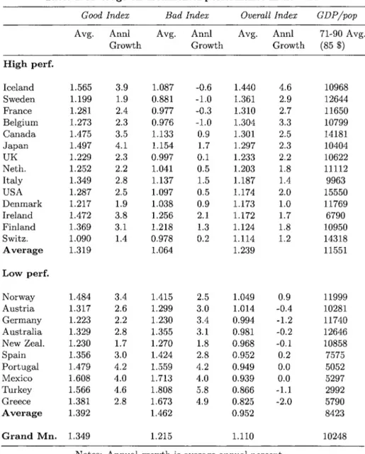
Leaving aside t h e disaggregated outcomes obtained using t h e method-ology described above, in Table 1 below we provide t h e average values. In Table 1, for each index, t h e first columns show t h e geometric mean of t h e index between 1971 and 1990 and measure t h e average performance of an individual country with respect to t h e base year 1971. T h e second columns are reserved for t h e average annual growth rate of each index. Our comparative analysis will be based on t h e average performance indi-cators evaluated with respect to t h e base year. Starting from the b o t t o m of t h e table, t h e mean environmental performance index (overall index), averaged over all t h e countries in t h e sample, indicates t h a t over t h e years 1971-1990 O E C D countries could have successfully expanded their desirable o u t p u t to undesirable o u t p u t ratio by 1 1 % . T h e good out-p u t quantity index averages 34.9% and t h e bad o u t out-p u t quantity index averages 21.5%. Individual country performances indicate t h a t , while Iceland, Sweden and France were t h e leaders in expanding their good o u t p u t over t h e bad o u t p u t s , Mexico, Turkey and Greece were t h e worst
•^"^Note that this index measures the environmental performance of each country relative to itself in 1971. Its advantage is that it does not require any assumptions about cross country technology. However, if the interest is in the cross-country comparisons of environmental efficiency levels, one can assume the same technology for all the countries and let /c = 1,...., /C index the countries in the sample. Then, a reasonable benchmark would be a hypothetical country constructed as the mean of the data, and the resultant efficiency scores will provide a cross country comparison relative to the mean. See Fare, Grosskopf and Hernandez-Sancho (2004) for an alternative approach in their application.
Essay 2:Environmental Performance 85
performers in this respect.
It is well known t h a t during t h e past two decades the developed coun-tries have m a d e i m p o r t a n t efforts in reducing emissions of pollutants. However, as t h e results in Table 1 suggest, these have not been equally i m p o r t a n t for all O E C D countries. In this regard, t h e classification of countries into those t h a t performed b e t t e r t h a n average and those below t h e average with respect to t h e overall environmental performance indi-cator sheds light on t h e relative importance attached t o environmental concerns while pursuing growth objectives.
A comparison of t h e average indicators reveals t h a t relatively low in-come countries, as measured by average per-capita G D P between 1971-1990 expressed in international prices (1985 U.S. dollars), while trying to catch-up with relatively high income countries may have ignored en-vironmental concerns. Note t h a t while these countries achieved higher growth rates for t h e good o u t p u t t h a n high income countries, their emis-sions of pollutants have increased at an even faster rate, lowering their environmental performance below 1971 levels. T h e relatively high in-come countries are t h e ones which achieved lower t h a n average growth in good o u t p u t with rather low (and in 5 cases with negative) growth rates in bad o u t p u t (again evaluated with respect to the base year 1971). This is an indication t h a t environmental concerns are becoming a bind-ing constraint only after a certain level of income is reached and this can be best addressed in an Environmental Kuznets Curve context us-ing panel data, to which we t u r n next.
Letting En represent the environmental performance of country i in year ^, t h e equation below specifies a possible relation between environ-mental performance and per-capita G D P ( G D P P C ) :
Bit = Pu + f32GDPPCu + (33{GDPPC)l + ^^{GDPPC)l + eu
where: i: country index; t: time index; e: disturbance t e r m with mean zero and finite variance. T h e shape of t h e polynomial will reveal t h e relationship between environmental efficiency and G D P per capita. A negative sign for G D P P C coupled with a positive sign for its quadratic and a negative sign for its cubic terms will imply deteriorating environ-mental performance at t h e initial phases of growth which is followed by a phase of improvement and t h e n a further deterioration once a critical level of per capita G D P is reached.
Table I. A v e r a g e environmental performance Indicators H i g h perf. Iceland Sweden France Belgium Canada Japan UK Neth. Italy USA Denmark Ireland Finland Switz. A v e r a g e Low perf. Norway Austria Germany Australia New Zeal. Spain Portugal Mexico Turkey Greece A v e r a g e Grand M n . Good Index Avg. 1.565 1.199 1.281 1.273 1.475 1.497 1.229 1.252 1.349 1.287 1.217 1.472 1.369 1.090 1.319 1.484 1.317 1.223 1.329 1.230 1.356 1.479 1.608 1.566 1.381 1.392 1.349 Notes: Annl Growth 3.9 1.9 2.4 2.3 3.5 4.1 2.3 2.2 2.8 2.5 1.9 3.8 3.1 1.4 3.4 2.6 2.2 2.8 1.7 3.0 4.2 4.0 4.6 2.8 Bad Index Avg. 1.087 0.881 0.977 0.976 1.133 1.154 0.997 1.041 1.137 1.097 1.038 1.256 1.218 0.978 1.064 1.415 1.299 1.230 1.355 1.270 1.424 1.559 1.713 1.808 1.673 1.462 1.215 Annual growth is Annl Growth -0.6 -1.0 -0.3 -1.0 0.9 1.7 0.1 0.5 1.5 0.5 0.9 2.1 1.3 0.2 2.5 3.0 3.4 3.1 1.8 2.8 4.2 4.0 5.8 4.9 Overall Index Avg. 1.440 1.361 1.310 1.304 1.301 1.297 1.233 1.203 1.187 1.174 1.173 1.172 1.124 1.114 1.239 1.049 1.014 0.994 0.981 0.968 0.952 0.949 0.939 0.866 0.825 0.952 1.110 Annl Growth 4.6 2.9 2.7 3.3 2.5 2.3 2.2 1.8 1.4 2.0 1.0 1.7 1.8 1.2 0.9 -0.4 -1.2 -0.2 -0.1 0.2 0.0 0.0 -1.1 -2.0
average annual percent.
GDP/pop 71-90 Avg. (85$) 10968 12644 11650 10799 14181 10404 10622 11112 9963 15550 11769 6790 10950 14318 11551 11999 10281 11740 12646 10858 7575 5052 5297 2992 5790 8423 10248
Models that combine cross-section and time-series data rely on the premise that differences across units can be captured in differences in the intercept term. However estimation techniques differ with respect to the nature of assumptions made on the intercept of the equation. If the Pii are assumed to be fixed parameters, then the model is known as
Essay 2.'Environmental Performance 87
a fixed effects model. If on t h e other hand t h e Pu are assumed to be r a n d o m variables t h a t are expressed as Pu = /5i + /^i, where /?i is an unknown parameter and fii are independent and identically distributed r a n d o m variables with mean zero and constant variance, then the model is called a r a n d o m effects model. T h e disadvantage of t h e fixed effects model is t h a t there are too many parameters to be estimated and hence loss of degrees of freedom which can be avoided if we either assume t h e same intercept for all t h e cross sectional units, or assume Pu to be ran-dom variables. Nevertheless, t h e r a n d o m effects model is not totally free from problems. In cases where fii and other independent variables are correlated, the r a n d o m effects model is similar to an omitted variable specification which will lead to biased parameter estimates, making a fixed effects model a more appropriate choice. In examining t h e rela-tionship between our environmental performance index and per-capita GDP, we will perform t h e relevant tests to determine t h e most suitable estimation form.
Table 2 below provides t h e parameter estimates of t h e regressions for t h e E index under alternative specifications where column one and two provide t h e parameter estimates of t h e fixed effects model with a com-mon intercept and fixed effects model with country specific intercepts respectively. T h e third column is reserved for t h e parameter estimates of t h e r a n d o m effects model. An F test performed on t h e alternative specifications of the fixed effects model rejects the null hypothesis of a common intercept in favor of t h e model with country specific intercept terms. Furthermore, t h e choice between the fixed effects model and the r a n d o m effects model can be made using t h e Hausman test. T h e Haus-m a n test has an asyHaus-mptotic xfk-i) distribution and in this particular case we fail to reject t h e null hypothesis which suggests t h a t the r a n d o m effects model is the appropriate specification.^^ So our preferred model is t h e r a n d o m effects model.
T h e most apparent outcome in all t h e specifications of t h e model is t h a t G D P per capita, its quadratic and cubic terms are always statisti-cally significant and their respective signs imply deteriorating environ-mental performance at the initial phases of growth (up to an income
•"•^Hausman test statistics test for the orthogonahty of the random effects and the regressors, i.e., Ho : E{^i\xit) = 0. Failure to reject this null, is failure to reject no correlation between
/j.i and regressors. In this case the preferred specification is the random effects model since
the random effects estimator is a best linear unbiased estimator once HQ is satisfied. Our test statistic xf^) = 2.665 is less than the critical value 7.82 at 5% significance level and fails to reject the null hypothesis.
level of approximately $6000 according to both the fixed effect model and the random effects model) which is followed by a phase of improve-ment and then a further deterioration once a critical level of per capita GDP (approximately $21000) is reached. This is actually another rep-resentation of the environmental Kuznets curve relationship where the initial deterioration of environmental conditions and its improvement in latter stages of economic growth manifest itself as an initial decline and then an improvement of environmental efficiency as measured by our index. The upper turning point is slightly beyond the sample range indicating that there may be negative repercussions on environmental performance after this level of income is reached^^
How do these results compare to those obtained in other studies? Di-rect comparisons are difficult since our index is a composite one which includes both carbon dioxide and soHd particulate matter, while other studies reported results for each pollutant individually. Studies almost unanimously agree that carbon dioxide emissions are monotonically in-creasing with income. For solid particulate matter, results reported vary from steadily declining emissions in Grossman and Krueger (1995) to improving environmental conditions after $11217 per capita GDP in Selden and Song (1994) and $4500 in Panayotou (1993). Our results, which simultaneously account for carbon dioxide and solid particulate matter, suggest that environmental performance deteriorates until per capita income reaches approximately $6000, i.e., our turning point falls between the Selden and Song (1994) and Panayotou (1993) estimates.
6.3 Concluding Remarks
In this section we employed an index number approach to measure environmental performance in OECD countries between 1971 and 1990. This approach, which relies on the construction of a quantity index of good outputs and a quantity index of bad outputs by putting due em-phasis on the distinctive characteristics of production with negative ex-ternalities, provides a means of simultaneously accounting for multiple
^^When a Kuznets curve is sought over an alternative environmental performance index for which the computation strategy is described in footnote 7, this provides additional insight on the robustness of the results. A pooled regression of type Eu = /?ti + l32GDPPCti +
/33{GDPPC)^^ + /34{GDPPC)^^-\-eti where the constant term now captures any year specific
effects on this alternative environmental performance index, yields the same 'sign ordering'
as in regressions in Table 1 for the (quite significant) parameter estimates. The relevant
hypothesis test, by rejecting any year specific effects, favors a common intercept model. The turning points with this new specification are $7439 and $15925.
Essay 2.'Environmental Performance 89 Table 2 Parameter estimates for alternative models
Environraental Performance Index
Constant Intercept Fixed Effects'" Random Effects Constant GDPPC (GDPPC)^ (GDPPC)^ R 2 ^ R^^ Homogeneity test (DF)
Hausman test stat. (DF) Turning Points N 0.9726 (14.201) -3.96E-05 (-1.514) 7.29E-09 (2.445) -2.05E-13 (-1.950) 0.275 0.938 $3129 $20578 480 1.5088 -0.000232 (-7.231) 2.45E-08 (7.687) -6.01E-13 (-5.959) 0.687 0.968 25.39 (23, 453) $6107 $21069 480 1.436 (6.896) -0.000203 (-3.349) 2.18E-08 (3.810) -5.30E-13 (-3.074) 0.684 0.661 2.665 (3) $5998 $20925 480 "^ Constant terms include the mean of the estimated country effects. ^ R^ of the unweighted regression.
"" R^ of the weighted regression.
pollutants within a production theoretic framework.
Our results suggest t h a t efforts in reducing emissions of pollutants have not been equally important for all O E C D countries; relatively low income countries are generally lagging behind high income countries in this regard. While lower income countries achieved higher growth rates on average for t h e good o u t p u t t h a n high income countries, their emis-sions of pollutants have increased at an even faster rate, lowering their environmental performance below 1971 levels.
A formal analysis t h a t establishes the link between economic growth and environmental performance reveals t h a t there exists a critical level of per capita income of approximately $6000 above which environmental
performance increases. This result provides further evidence for the existence of an environmental Kuznets type relationship between per capita GDP and our environmental index which simultaneously accounts for multiple pollutants.
7. Remarks on t h e Literature
The notions of weak disposability and null-jointness may be traced back to Shephard and Fare (1974). See also Fare and Grosskopf (1983a,b) for early efforts at measuring congestion and modeling output sets with byproducts; these early efforts typically employed Shephard type dis-tance functions. Fare, Grosskopf, Lovell and Pasurka (1989) struggled with alternate nonparametric specifications of performance measures in the presence of undesirable outputs, including a hyperbolic measure that is very close to the directional distance function which was not employed in this literature until later. Similarly, Fare, Grosskopf, Lovell and Yai-sawarng (1993) used Shephard type distance functions as a basis for shadow pricing undesirable outputs.
The directional distance function approach to modeling and measur-ing performance in the presence of undesirable outputs may be traced back to a series of theoretical and empirical papers and a dissertation by Y.H. Chung. See Chambers, Chung and Fare (1998) and Chung, Fare, and Grosskopf (1997). The shadow price model based on direc-tional distance functions is discussed in Fare and Grosskopf (1998) and has been applied in Ball, Fare, Grosskopf and Nehring (2001) and Fare, Grosskopf and Weber (2001a,b).
Although not discussed in detail in this essay, some work has been done on modeling the effects of regulation on profitability, particularly in the nonparametric, DEA framework, see Brannlund, Fare and Grosskopf (1995). Brannlund, Chung, Fare and Grosskopf (1998) extend this model to simulate introduction of emissions trading in the Swedish pa-per and pulp industry.
The network model approach includes the early paper included here by Fare, Grosskopf and Lee. See Fare and Grosskopf (1996) for a general discussion of network models.
8. Appendix: Proofs
Proof of (2.21) Assume that