USING MIXTURE COPULA FOR THE CALCULATION
OF VALUE AT RISK: DOLAR-EURO PORTFOLIO
(MSc. Thesis)
DEMET ÇATAL
SUPERVISOR: Asst.Prof. Dr. RAİF SERKAN ALBAYRAK
Department of Actuarial Sciences
Bornova,İZMİR 2013
YASAR UNIVERSITY
GRADUATE SCOOL OF NATURAL AND APPLIED SCIENCE
(MSc. Thesis)
USING MIXTURE COPULA FOR THE CALCULATION
OF VALUE AT RISK: DOLAR-EURO PORTFOLIO
Demet ÇATAL
Thesis Advisor: Asst.Prof. Dr. Raif Serkan Albayrak
Department of Actuarial Sciences
Bornova,İZMİR 2013
This study titled “Used mixture copula for calculating of value at risk: dolar-euro portfolio” and presented as master thesis. Thesis by Demet Çatal has been evaluated in compliance with the relevant provisions of Y.U Graduate Education and Training Regulation and Y.U Institute of Science Education and Training Direction and jury members written below have decided for the defence of this thesis and it has been declared by consensus / majority of votes that the candidate has succeeded in thesis defence examination dated 29/07/2013
Jüri Members: Signature Yrd.Doç.Dr. RAİF SERKAN ALBAYRAK
Yrd.Doç.Dr. BANU ÖZAKÇAN ÖZGÜREL Yrd.Doç.Dr. DİLVİN TAŞKIN
ÖZET
Riske Maruz Değer (RMD) hesaplamalarında portföyü oluşturan değerlerin bağımlılık yapılarının formu modelin performansı üzerinde büyük öneme sahiptir. Bu çalışmada yatırım araçlarının bağımlılık yapılarının bir çok formda modellenmesine olanak veren kopula çeşitleri, Dolar ve Euro portföylerinde incelenmiştir. İki yatırım aracının bağımlılık yapılarının negatif ve pozitif getiri bölgelerinde farklılık göstermesi nedeniyle bu bölgelere yönelik kopula karışımı önerilmiştir. Geleneksel metotlar, kopula fonksiyonları ve önerilen karışım kopulanın performansları geri dönük test ile ölçümlenmiştir. Türkiye’de döviz endeksleri üzerinde kopula alanında bir çalışma yapılmamış fakat hisse senetleri, bonolar ve hayat sigortası poliçeleri üzerinden modellemeler yapılmıştır.
ABSTRACT
Dependence structure set up of financial assets has substantial importance in the performance of Value at Risk calculations. In this article, copula variations that allow modeling of rich dependency structures of financial assets, in particular of Dollar - Euro portfolios are examined. Due to significant dependency regime differences in positive and negative returns, adoption of regional copula mixture is proposed. Performances of traditional VaR calculation methods, copulas and mixture copulas are compared by back testing. Although copulas have been applied to stock returns, bonds and life insurance policies, until now there have been no copula studies related to exchange rates for Turkish markets.
ACKNOWLEDGEMENTS
I would like to express my deepest gratitude to my supervisor Asst.Prof. Dr. Raif Serkan Albayrak for his friendship, guidance, advice, motivation, encouragements, patience and insight throughout my thesis process.
I would like to thank to Asst.Prof. Dr. Banu Özakcan Özgürel for guiding me through the earlier part of my master studies and for her continued support throughout my master.
I would like to thank to Asst.Prof. Dr. Dilvin Taşkın for sharing her precicious comment that substancial input the discussion impoved in my thesis.
In addition, I would like to express my endless gratitude to my dear family and to all my friends for their endless support, love and encouragement. Thesis is dedicated to my family…
TEXT OF OATH
I declare and honesly confirm that my study titled “used mixture copula for calculating of value at risk: dolar-euro portfolio”, and presented as Master’s Thesis has been written without applying to any assistance inconsistent with scientific ethics and traditions and all sources I have benefited from are listed in bibliography and I have benefited from these sources by means of making references.
29/07/2013
Adı SOYADI Signature DEMET ÇATAL
TABLE OF CONTENTS ÖZET ... iv ABSTRACT ... v ACKNOWLEDGEMENTS ... vi INDEX OF FIGURE ... x INDEX OF TABLES ... xi 1. INTRODUCTION ... 1 2. METHODOLOGY ... 5 2.1. Value At Risk ... 5
2.1.1. Value at risk approaches ... 6
2.1.2. Historical simulation ... 7
2.1.3. Variance-covariance method ... 7
2.1.4. Monte Carlo simulation ... 8
2.2. Backtest Methods ... 10
2.2.1. Pearson ( ) goodness of fit test ... 10
3. COPULA ... 12
3.1. Basic Features Of Copulas ... 13
4. FAMILIES OF COPULA ... 19
4.1. Eliptical Copula ... 19
4.1.1. Normal (Gaussian) copula ... 19
4.1.2. T copula ... 21
4.2. Archimedian Copula ... 22
4.2.1. Clayton copula ... 25
4.2.3. Gumbel copula ... 26
4.3. Gaussian Mixture Copula... 26
5. APPLICATION OF COPULA MODELLING ... 28
5.1. Data ... 28
5.1.1. Historical simulation ... 29
5.1.2. Maximum likelihood estimation ... 32
5.1.3. Hull-White copula ... 34 5.1.4. Normal copula ... 38 5.1.5. T copula ... 42 5.1.6. Clayton copula ... 44 5.1.7. Frank copula ... 47 5.1.8. Mixture copula ... 50 6. CONCLUSION ... 60
6.1. Pearson Goodness Of Fit Test ... 60
BIBLIOGRAPHI ... 69
APPENDICES ... 72
INDEX OF FIGURE
Figure 1: Frechet-Hoeffding upper bound W(u1,u2) (upper panel), product copula (u1,u2) (middle panel), Frechet-Hoeffding lower bound M(u1,u2) (lower panel).
... 18
Figure 2: The graphs of normal copula... 21
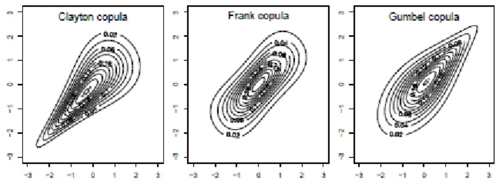
Figure 3: The Clayton and Gumbel and, Frank Copula are based on Normal margins. ... 26
Figure 4: Histrogram of the returns of the portfolio of (X1 and X2). VAR is represented with the vertical line (in red color). ... 30
Figure 5: The graphic of the Dollar-Euro alteration returns ... 31
Figure 6: The distribution of the portfolio prepared for the historical data ... 32
Figure 7: The x values recieves for maximum likelihood estimation method and marginals... 33
Figure 8: The distributions of the copula values that have been formed using the Hull-White method ... 38
Figure 9: The dependency model of the values constructed by normal copula ... 42
Figure 10: Dependency model of the values constructed by Student-t copula... 44
Figure 11: Dependency model of the values constructed by Clayton copula... 47
Figure 12: The dependency model of the values constructed by Frank copula... 50
Figure 13: A distribution graph of US Dollar and Euro returns ... 50
INDEX OF TABLES
Table 4 1 : Table with the most important generators ... 24
Table 6 1 : Result of R for all methods ... 63
Table 6 2 :Exceptional date numbers for all methods ... 64
Table 6 3 : Result of all methods ... 65
Table 6 4 : Goodness of Fit chi-square(1) values ... 66
1. INTRODUCTION
Globalization in the recent years, availability of a number of new products in the financial markets with the technology and increase in the competition between the financial corporations have caused a remarkable increase in the risk factors. The increase of the interaction in the financial markets, the rapid change of the market conditions have caused extreme fluctuations of the prices. These changes and fluctuations makes the financial corporations all around the world open to risks and it makes the risk management gain importance. Today, many organizations want to know how big risk position it has against the financial developments. Perhaps, the best answer to this question can be given by means of “Value at Risk” method.
In financial mathematics and financial risk management, Value at Risk (VAR) is the estimation method of the maximum loss of a portfolio or asset under certain assumptions, that describes a certain confidence interval for a certain period. The methods used in VAR calculation are grouped under titles of parametric and non-parametric methods. Particularly, in the calculation of VAR for portfolios, the relations of the assets forming the portfolio is known to be an important factor in determining the overall risk. In cases where dependence structure of returns of assets with each other is linear, the standard statistical methods can be used in VAR calculation. In this thesis, copula method which gives opportunity to model the dependency structures of investment tools in many forms especially in situations when the financial markets has non-linear portfolios due to extreme fluctuations are analyzed. On the other hand, when the structure of dependence between asset returns is in a form other than the linearity, we do not have the opportunity to express that depence with a single statistical parameter such as the correlation coefficient. Copulas are often used in modeling of dependence forms in many different areas recently (Nelsen, 2006). Dependence structures are extremely important in risk calculations and increasing rates of copula
applications may be found in financial literature (Cherubini, Luciano and Vecciato, 2004).
The word copula is a Latin word and it means “connection, relation”. It was used in mathematical and statistical meaning by Abe Sklar for the first time in 1959 while defining one-dimensional distribution functions in multidimensional form to mean “moving together”. The most important outcomes regarding the copulas occur during the development period of this theory continuing from 1958 to 1976. Sklar show that there is a relation between the copulas and the random variables in his article published in 1973. In short, even copula functions entered the literature in 1959, especially their statistical characteristics and applications are still being developed today.
Copula is defined as dependency function between the random variables. Copulas, with a more certain meaning, are the functions that relates the marginal distributions with their multivariable distributions. In fact, copula functions enable to separate the marginal distributions of the variables and identify the dependency structures clearly. In this way, single variable techniques can be used and a direct connection can be provided with the nonparametric dependency measures. Besides, the deficiencies of the linear correlation technique which is well-known and used up to now can be avoided.
Today, the relation between copula functions and finance is one of the most significant methodologies used to gather the variables studied in finance and the risk factors effective on the markets. As the data is gathered by using the statistical theory due to the indecisive, irregular and temporary attitudes in the financial market, this subject has gained importance for the people working in the application field of finance and the academicians and it has replaced some of the standard subjects used in the mathematical finance. None of the researchers today examines a statistical or financial problem regarding the financial markets without considering the problem of aberration. When the problems like pricing and risk measurement are one-dimensional, effective results can be obtained from the models founded out of the normality hypothesis but when the problem is
multi-dimensional, the models that are founded without using this hypothesis have many mistakes.
Copula use in VAR calculation depending on the characteristics of the related financial market can lead to the possibility of a non-return confusion in risk calculations, but the use of it providing high productivity can also be seen. Therefore, successful practices of copulas in the calculation of risk in some markets do not mean that they will show a similar success in other markets. For this reason, in literature market specific dependency structures formed according to the market qualities that requires the use of different forms of copula.
Two studies have been found regarding Turkey market in the literature. In Çifter and Özün’s study (2007), the value at risk of the values is predicted with the methods of delta normal, EWMA, correlation with dynamic conditions and conditional symmetric joe-clayton copula with the daily interest rate of Turkish Lira and value at risk belonging to a portfolio weighed equally consisting of a daily US Dolar/TL exchange rate. In addition, modelling with copula of the interrelation with investment fund strategies and one application in Turkey are one of the studies held in this field. Avutman (2011) stopped at the investment funds in her thesis ad by modelling with copula the funds formed up in two different strategies and two types belonging to Finansbank, she examined the copula structure in them. Although copulas have been applied to stock returns, bonds and life insurance policies, until now there have been no copula studies related to exchange rates for Turkish markets.
In literature, the values are produced by Monte-Carlo simulations from the dependency structures modeled with copula, these values are multiplied with weights determined in portfolio and VAR calculation is performed through the distribution of returns of the portfolio according to the account percentile (Ray, 2011). In summary, copulas are used to fine-tune the calculation of VAR through simulation.
In this thesis a model is developed with the parametric method used in the calculation of VAR enhanced with the copula. This model is operated with assets like Euro and the Dollar versus TL exchange rates that are most commonly used in the portfolios of the Turkish financial market and compared using the other methods of calculating VAR with Backtest methods. In the next section of this thesis, respectively, Value at Risk calculation methods without using copula, the backtest method, and general forms of copulas are briefly reviewed. The next section summarizes the use of the copula in VAR calculation with the simulation method. In the fourth chapter, the model developed in this thesis, using the mixture copula in VAR parametric calculation is described. The fifth section contains a comparison of different methods of VAR and final section concludes the thesis.
2. METHODOLOGY
2.1. Value At Risk
VAR analysis methods allows the direct calculation of the risk of a single investment instrument, as well as the portfolios consisting of more than one investment tool and is able to direct the investor's investment processes.
VAR is fundamentally used in banks with large trading portfolios where risk management is mandatory, pension funds, other financial institutions, regulatory bodies that are involved in monitoring and control activities of the industry , and non-financial institutions that are exposed to financial risk because of the financial instruments held by them (Jorion, 2000). The VAR usage areas in these institutions can be classified into three categories: passive use in terms of measuring and reporting of total risk, the defensive use where risk control is made by determination of position limits and consequently, through determining risk; finally, the active use in terms of risk management (Dowd, 1998).
We see the emergence and development of VAR techniques in financial risk management after the financial scandals in the early 1990s. The measurement of market risk by using VAR method in the field of finance of Turkey is set to the mandatory in new Banking Law which came into force in 1999, with the risk management and internal control systems.
In determining risk measurement methods; the return on the portfolio, returns of financial assets composing of portfolio and direct dependence are between most important factors. The biggest advantage of VAR is expressing the different positions in a single monetary value by taking into account the dependence usually expressed in correlations between risk factors.
The VAR values are meaningless without time zone and confidence levels. Because the investors trade with active portfolios, financial companies prefer a typical day time period, and institutional investors and non-financial corporations prefer long periods (Linsmeier J. & Pearson N.D., 1996). Because confidence level selection can be determined depending on the purpose while assessing capital requirements, managers who do not like taking risk can opt for a higher level of confidence.
Symbolically, the VAR calculation is expressed by the formula =( ) ). Here, α reflects the chosen confidence level , reflects corresponding to the value of α probability of the standard normal distribution, the portfolio average returns, σ risk of returns , and W reflects the value of the initial portfolio (Jorion, 2001).
Accordingly, when the initial portfolio value is 1 million, the annual return of the portfolio is 15%, the risk of the portfolio is 10% and 99% confidence level, 25-day VAR calculation gives the following result:
=( -2.33*%10*√ )*¨1M= ¨ 76,318
A year is assumed to be 250 trading days in the square root in the formula. According to this result, the likelihood of a loss lower than 7.63% is under one percent level. As it can be seen under the assumption of normality, the VAR calculation is very simple.
2.1.1. Value at risk approaches
In Value at Risk calculation, when parametric models are based on the statistical parameters of the risk distribution factors, the non-parametric models are divided into two as historical and simulation model (Ammann M. & Reich C., 2001). When price movements do not fit the normal distribution, methods based on simulation give healthy results because of the difficulty in VAR calculation methods and the unique possibility of expected changes for portfolios with different return distributions (Bolgün K. & Akcay M.,2005). In this section, the
three most common methods for calculating VAR, historical simulation, variance-covariance approach, and Monte Carlo simulation are summarized.
2.1.2. Historical simulation
Historical simulation is a simple, a theoretical approach that requires relatively few assumptions about the statistical distributions of the underlying market factors. In this approach, the VAR for a portfolio is estimated by creating a hypothetical time series of returns on that portfolio, obtained by running the portfolio through actual historical data and computing the changes that would have occurred in each period. Historical simulation approach estimates VAR and other risk measures using past observations of return and loss data. This approach is realized by tracking the history of price changes for all portfolio components and applying exactly the same movements to the underlyings for the target period. Historical simulation method is widely used, which can be explained by its easy implementation and fast calculations. Another advantage of this approach is its compliance to the regulators requirements.
Historical Simulation has obvious weaknesses. First, this method does not rest upon a probabilistic setup. Second, historical data may not be an adequate indication for the current economic agenda. Finally third, this method requires immense amount of data which is often not available.
2.1.3. Variance-covariance method
Variance-covariance method is an approach that has the benefit of simplicity but is limited by the difficulties associated with deriving probability distributions. In variance-covariance method of estimation of VAR, it assumes the returns (X) are normally distributed. It requires that we estimate first two moments i.e. mean and standard deviation σ which completely describe the normal distribution . Therefore, 99% =( ) ) i.e. μ-2.33*σ (where Pr( (X- μ )/ σ < Zα)=.01) (Jorion, 2001).
In the parametric methods used in VAR calculations, it is assumed that the financial asset income and portfolio risk have a normal distribution, and they are in a linear relation with the risk factors. In these methods, basic parameters consisting of standard deviations gathered from the past return series of the portfolio and the correlation are calculated to calculate variance and covariance matrix and the expected losses can be predicted by calculating the VAR of portfolio according to this. Different assumptions regarding the return distribution changes the VAR formula. That is to say, when return distribution is assumed log-normal with the same parameters of the sample above (15% average and 10% risk);
( √
)
a respectively lower VAR value is calculated. A similar logic works when a different probability model is assumed for return distribution. In this situation, the parameters of the assumed model are found with mostly likelihood estimation method.
2.1.4. Monte Carlo simulation
In modern financial risk management, one fundamental quantity of interest is value at risk (VAR). It denotes the amount by which a portfolio of financial assets might fall at the most with a given probability during a particular time horizon. For the sake of simplification we will only consider time horizons of one week length in this thesis. This covers portfolios that include assets that can be sold in one week. The discussions would have to be modified slightly if we were interested in longer time horizons.
Monte Carlo simulation method is used in VAR calculations of the complex portfolios including the financial assets having a nonlinear return structure like options (Morgan, 1996). Monte Carlo simulation is similar to the historical simulation; when historical simulation uses the real data to create
estimation portfolio return and loss, Monte Carlo simulation uses the unreal rational values by choosing a statistical distribution reflection the possible changes in the prices (Duman, 2000).
We present general information on how to compute the VAR of a portfolio using Monte Carlo simulation. The value of the portfolio at present time t will be denoted by Vt. Let us assume that Vt depends on n risk factors such as (relative) interest rates, foreign exchange (FX) rates, share prices, etc. Then a Monte Carlo computation of the VAR would consist of the following steps:
1. Choose the level of confidence 1 − α to which the VAR refers.
2. Simulate the evolution of the risk factors from time t to time t+1 with appropriate marginal distributions and an appropriate joint distribution that describe the behaviour of the risk factors. The number m of these n-tuples has to be large enough (typically m = O(1000)) to obtain sufficient statistics in step 5. 3. Calculate the m different values of the portfolio at time t + 1 using the values of the simulated n-tuples of the risk factors. Let us denote these values by
.
4. Calculate the simulated returns and losses, i.e., the differences between the simulated future portfolio values and the present portfolio value, = for i = 1, . . . ,m.
5. Ignore the fraction of the α worst changes . The minimum of the remaining s is then the VAR of the portfolio at time t. It will be denoted by VAR(α, t, t + 1). As soon as the time evolves from t to t+1, the real value of the (unchanged) portfolio changes from to . With this data at hand, one can backtest VAR(α, t, t+1) by comparing it with = .
The power of Monte Carlo simulation is due to not making normality estimation for the income. Even the estimations of the predictions are made by using the historical data, subjective data and other information can be easily
implemented to the system. On the other hand, wrong estimations regarding the pricing models and basic stochastic durations can cause to calculate VAR lower or higher than it really is.
2.2. Backtest Methods
To measure the performance of VAR techniques which is used as a tool for standard risk measurement by both financial institutions and non-financial institutions today, the backtest methods may be used. Therefore, the approval of the model is performed by to subject it to VARious tests and evaluation of results. A backtest compares the VAR model values calculated with realized gains and loss values of portfolios and tests the accuracy of the VAR model. Then exception days which the value of the selected confidence level that VAR model proposed is higher than the daily loss are counted. Also, such tests are known as termless coverage tests (Jorion, 2001). In particular, to measure the performance of risk measurement models that they use, banks have to determine the deviation number by comparing portfolio returns and risk measurement models with value figures at estimated daily risk.
In this section, backtest methods used for VAR models; Pearson Chi-Square ( ) goodness of fit test is summarized.
2.2.1. Pearson ( ) goodness of fit test
Pearson's chi-square test was developed by the British statistician Karl Pearson in the 1900.
Chi-square goodness of fit test of VAR models are based on the differences between observed and expected frequencies of the data.
Consider a sample of independent observations of size n with unknown F (y, ), is the parameter vector, an example of sample, connected
in the form of an example of Labour was formed independent observations is assumed that F (y), coincidence that the true but unknown cumulative distribution function and the origin of (Y) the theoretical cumulative normal distribution function to describe;
( ) ( ) ( ) ( ) There is in the form of hypotheses to be tested.
If observations, the sampleand standard deviation and mean
return the form, , the asymptotic N (0,1) distributed. In this case, statistic test, ∑ ( )
is obtained.
is Pearson's cumulative test statistic and computed under the hypothesis of asymptotic value chi-square distribution of degree of freedom (Dong and Giles, 2004). , i. the expected probability of observations per class, , expected frequencies, k, n the number of clusters in the data, and , refers to the observed frequencies.
3. COPULA
Traditional representations of multivariate distributions assume that all random variables have the same marginal distribution. In this representation, the dependence structure between the variables are expressed by the correlation coefficient. This approach may fall short of the dependency structures of investment instruments. The purpose of the analists making financial modeling is providing clearer results of VAR calculations by specifying a joint distribution with well-known functional forms. When these functional forms are connected with the help of copula, non-linear cross-dependencies between asset returns, thick tail, and even unusual effects can be modelled.
Because copula can capture dependency structures regardless of the forms of the marginals, it provides great flexibility for the covariance structure modeling, accordingly determining the dependency structures forming the portfolio in VAR calculations. As we will see, the main advantage of copula functions is that they enable us to tackle the specification problem of marginal univariate distributions separately from the specification of market co-movement and dependence. Using a copula to build multivariate distributions is a flexible and powerful technique, because it separates choice of dependence from choice of marginals on which no restrictions are placed.
There are many resources that can be used about the theoretical background and characteristics of copulas. For example, Nelsen (2006) described mathematical properties and derivations of copulas in general. In the same resource, simulation algoritms of multivariate distributions produced by using copula are also compiled. In the literature, Embrechts, Lindskog and McNeil (2003) provides example applications of general copula in the finance field. In addition, Cherubini, Luciano and Vecchiato (2004) examines the use of a copula for capital portfolio approach. They also commented about the time-varying correlation in the same study. Li (2000) arranged the correlation structure of financial assets with the Gaussian copula. Name of Gaussian copula stems from determining the variables of dependence structure as well as multivariate normal distribution with binary correlation parameter. However, Li(2000) didn’t use the normal distribution for marjinal distribution of assets. Gaussian and Frank copula
can not be used for modeling dependency structures of extreme values of assets; for this purpose Gumbel copula for the right tail and the Cook - Johnson copula for left tail are used. Cherubini and Luciano (2001) estimated VAR by using the Archimedean copula and the historical data constructed from the marginal distributions. Fortin and Kuzmics (2002) used a convex linear combination of copulas for VAR estimation of a portfolio of FSTE and DAX exchange indices. Cherubini and Luciano (2001) used Archimedean copula to estimate the marginal distributions and VAR using the historical empirical distribution, Meneguzzo and Vecchiato (2002) used copula for risk modeling of credit derivatives. McNeil, AJ, Frey, R., and Embrechts (2005) provides comprehensive information for theoretical concepts and modeling techniques of quantitative risk management. This book is a practical tool for financial risk analysts, actuaries, regulators, or students of quantitative finance.
The mixture copula is usually used as a linear combination of copula for different correlation parameters in the field of finance and economics. It is a simple and flexible model to summarize the dependence structure. Hu (2003) used the mixture copula approach to measure pre-determined components dependence in the financial markets. The mixture copula was constructed by combining Gaussian, Gumbel and Gaussian survival copulas. Based on the Gaussian copula, calculating the dependency is achieved by combining two other copulas and the left and right tail along with traditional demonstration. In this case, because it was constructed more than one copula, mixture copula has a more flexible structure than one-dimensional copula. In addition, the mixture copula is defined as the linear combination of the maximum copula, independent copula and the minimum copula with Spearman's rho coefficient (Ouyang et al., 2009).
3.1. Basic Features Of Copulas
In this section we summarise the basic definitions that are necessary to describe fundamentals of copulas. We then present important properties of copulas that are needed in financial applications. At this point we refer to the textbook by Nelsen (2006).
Definition (Copula):A n-dimensional copula is a multivariate distribution, C, with Standard uniform marginal distributions(Nelsen, 2006).
A (n-dimensional) copula is the joint cumulative density function of a pair of variables (U; V ) with marginal uniform distributions on [0,1]. Thus a copula is a function C: → [0, 1] satisfying the following three properties:
1. [0, 1] C(1,1,1, … ,u, 1, 1, 1) = u,
2. [0, 1] , C( ,… , )= 0 if at least one of the equal zero,
3. C is grounded and n-increasing, i.e., the C-volume of every box whose vertices lie in is positive.
For the 2-dimensional case, these properties become; C(u, 1) = u and C(1, v) = v; u, v [0, 1],
C(u, 0) = C(0, v) = 0; u, v [0, 1],
, in [0, 1] such that < and < , we have: C( ) - C( ) - C( , ) + C( , ) 0
Condition 1 provides the restriction for the support of the variables and the marginal uniform distribution. Conditions 2 and 3 correspond to the existence of a nonnegative “density” function ( Wei Liu, 2006).
Copula is defined in the following theorem.
Theorem (Sklar): Let H be a joint distribution function with marginals , , … , . Then there exists an n-copula C such that for all x,y in ̅,
H( , , . . . , ) = C( ( ), ( ), . . . , ( )), for some copula C.
If , ,…, are all continuous then C is unique; otherwise C is uniquely determined on Ran *…* Ran , where Ran is the range of the marginal i. Conversely, if C is an n-copula and , , … , are distribution functions, then the function H defined above is an
n-dimensional distribution function with marginals , , … , ( Malevergne, Y. and D. Sornette, Extreme Financial Risks-2006).
It is shown in Nelsen (2006) that H has margins and that are given by
( ) ( ) and ( ) ( )
with Sklar’s Theorem, the use of the name “copula” becomes obvious. For a proof we direct the reader to Nelsen(2006), the standard introductory text on the subject. Example: Let H be a joint cumulative distribution function with margins F and G. Then, there exists a copula C such that H(x, y) = C[F(x),G(y)]; for any x, y.
For example Nelsen(2006) Farlie Gumbel Morgenstern(FGM) distribution; ( ) ( ) ( ) { ( ( )) ( ( ))} The copula of distribution clearly exists,
C(u,v)=u.v{1+ (1-u)(1-v)} -1< and u,v C( ( ), ( ))= ( )
If x and y independent random variables then the FGM copula with the same independence copula for α=0;
C(u,v)=u.v such that ( ) ( ) ( )=C( ( ), ( )).
Invariance theorem: If … has copula C, then = ( ), … , ( ); ( ); has the same copula C, if is an increasing function of . ( Malevergne, Y. and D. Sornette, 2006).
C( ( ), ( ) , … , ( )) = C( ( ( )), … , ( ( ))
By the invariance theorem, it can be seen that the copula is not affected by non-linear transformations of the random variables.
Copulas are very useful models for representing multivariate distributions with arbitrary marginals. One can model the marginal distributions of a multivariate distribution and find a copula to capture the dependence between the marginals.
F( ,…, ) = P {f( , … , ) = C( ( ), ( ),…, ( )) Once we find a copula for a multivariate distribution, we can interchange between the copula and the multivariate distribution environments. Thus working with copulas can be easier than working with multivariate distribution functions. For example if we want to simulate from a multivariate distribution, we can shift to the copula environment and simulate from the copula, then we find the corresponding random variates by transforming them back to the multivariate environment.
→ ( )) Random variable Cumulative function
F( , … , ) → C( ( ), ( ), … , ( )) Multivariate environment Copula environment
Due to the property that copulas are n-increasing, an upper and a lower bound can be found for any copulas. This situation explained by Frechet Bound limits.
Frechet bounds: We get Max(u + v – 1, 0) C(u, v) Min(u, v), where the lower bound indicates the largest negative dependence and the upper bound represents the largest positive dependence( Malevergne, Y. and D. Sornette,2006).
The upper bound corresponds to the copula of two variables X and Y in a deterministic increasing (nonlinear) relationship. Similarly the lower bound provides the copula of two variables in a deterministic decreasing (nonlinear) relationship. Moreover, two variables corresponding to Frechet upper
(respectively lower) bound are said to be comonotonic (respectively countermonotonic).
Notice that the correlation depends on the marginal distributions of the returns. The maximum value it can achieve can be computed by substituting the upper Fr´echet bound in the formula:
( )= ∫ ∫ ( ( ) ( ))
and the value corresponding to perfect negative correlation is obtained by substituting the lower bound
( )= ∫ ∫ ( ( ) ( ) )
Of course everyone would expect these formulas to yield = 1 and = −1. The news is that this is not true in general. We may check this in the simple case of a variable z normally distributed and which is obviously perfectly correlated with the first one, but has a chi-squared distribution.
Figure 1: Frechet-Hoeffding upper bound W(u1,u2) (upper panel), product copula (u1,u2) (middle panel), Frechet-Hoeffding lower bound M(u1,u2) (lower panel).
Copulas have a very simple structure. These copulas are very important as they represent some characteristic features. Then we introduce families of copulas. A copula family is defined by a copula function that includes an additional free parameter.
4. FAMILIES OF COPULA
Copulas play an important role in the construction of multivariate density function and, as a consequence, having at one’s disposal a variety of copulas can be very useful for building stochastic models having different properties that are sometimes indispensable in practice (e.g., heavy tails, asymmetries, etc.). Therefore, several investigations have been carried out concerning the construction of different families of copulas and their properties. Here, we present just a few of them, by focusing on the families that seem to be more popular in the literature (F. Durante and C. Sempi, 2009).
There are mainly two families of copulas used for financial applications: Elliptical Copulas and Archimedian Copulas. Eliptical copula was included Gaussian and student-t copula and Archimedian copulas was included Clayton, Gumbel, and Frank copulas are best known.
4.1. Eliptical Copula
The class of elliptical copula allow to model multivariate extreme events and forms of non-normal dependencies. Simulation from elliptical distributions is easy to perform. In this section we are going to present eliptical families of copulas. The most commonly used elliptical distributions are the multivariate normal and student-t distributions.
4.1.1. Normal (Gaussian) copula
The Gaussian (or normal) copula is the copula of the multivariate normal distribution. In fact, the random vector X=(X1, … , Xn) is multivariate normal iff: the univariate margins F1,…,Fn are Gaussians; the dependence structure among the margins is described by a unique copula function C such that:
where is the standard multivariate normal density function with linear correlation matrix R and is the inverse of the standard univariate Gaussian density function.
Multivariate normal is commonly used in risk management applications to simulate the distribution of the n risk factors affecting the value of the trading book (market risk) or the distribution of the n systematic factorsinfluencing the value of the credit worthiness index of a counterparty(credit risk).
If n=2, expression previous equation can be written as
where ρ is simply the linear correlation coefficient between the two random variables .
The bivariate Gaussian copula does not have upper tail dependence if ρ<1. Furthermore, since elliptical distributions are symmetric, the coefficient of upper and lower tail dependence are equal. Hence, Gaussian copulas do not even have lower tail dependence. (Malevergne, Y. and D. Sornette, 2006).
-1( ) 1( ) 2 2 Ga 1 2 2 2 1 2 C (u, v) = exp 2(1 ) 2 (1 ) v u x xy y dxdy
Figure 2: The graphs of normal copula
4.1.2. T copula
The copula of the multivariate t-Student distribution is the t-Student copula. Let X be a vector with an n-variate t-Student distribution with v degrees of freedom, mean vector μ (for v>1 ) and covariance matrix . It can be represented in the following way:
√ √
where μ , X~ and the random vector Z~ (0,Σ) are independent.
The copula of vector X is the t-Student copula with v degrees of freedom. It can be analytically represented in the following way:
)) ( ),..., ( ( ) ,..., ( 1 1 1 , 1 , v v k n v k k v u u t t u t u C
where √ for i,j where tk,vdenotes the multivariate d.f. of the random vector √ √ , where the random variable X~ and the random vector Y are independent. denotes the marginsof tn,v.
For n=2, the t-Student copula has the following analytic form:
where ρ is the linear correlation coefficient of the bivariate t-Student distribution with v degrees of freedom, if v> 2.
Unlike the Gaussian copula, it can be shownthat the t-Student copula has upper tail dependence. As one would expect, such dependence is increasing in ρ and decreasing in v. Therefore, the t-Student copula is more suitable than the Gaussian copula to simulate events like stock market crashesor the joint default in most of the counterparties in a credit portfolio.
The description of the t-copula relies on two parameters: the correlation matrix ρ as for the normal copula, and in addition the number of degrees of freedom v. An accurate estimation of the parameter v is rather difficult and this can have an important impact on the estimated value of the shape matrix. As a consequence, the t-copula may be more difficult to calibrate than the normal copula ( Malevergne, Y. and D. Sornette, 2006.)
4.2. Archimedian Copula
Every continuous, decreasing, convex function ϕ: [0, 1] → [0,∞) such that ϕ(1) = 0 is a generator for an Archimedean copula. If furthermore ϕ(0) = +1, then
) ( ( ) ( 2)/2 2 2 2 2 / 1 2 1 1 1 ) 1 ( 2 1 ) 1 ( 2 1 ... u tv tv uk v dxdy v y xy x the generator is called strict. Parametric generators give rise to families of Archimedean copulas.
An Archimedean copula can be written in the following form:
1
1 1
( ,..., n) [ ( ) ... ( )]n
C u u
u
uFor all and is a function often called the generator, satisfying
i) (1)=0;
ii) for all t (0,1), '
(t)<0 i.e is decreasing; iii) for all t (0,1), ''
(t)<0 i.e is convex.
For Archimedean copulas, the complexity of the dependence structure between n variables , usually described by an n-dimensional function, is reduced and embedded into the function of a single variable, the generator ϕ.(Malevergne, Y. and D. Sornette, 2006).
Every Archimedean copula behaves differently with respect to the tail dependence, a very important factor in dependence modelling. For these three copulas, their parameter ranges and the generators are given in Table;
name generator generator inverse parameter Clayton ( ) ( ) Frank ( ( ( )) ( )) ( ( ) ( ) ) ( ) Gumbel ( ) ( ( )) )
Table 4 1 : Table with the most important generators
As it has been already mentioned there is no analytical expression for the Spearman's rho for Archimedean copula. On the other hand, Kendall's tau can be computed with this formula (Genest and MacKay, 1986).
1 ' 0 ( ) 1 4 ( ) t dt t
Different coefficients for the left and right tail dependence are desirable in many models, where complex dependencies occur. The Gumbel copula exhibits higher correlation in the right tail, whereas the Clayton copula shows tighter concentration of mass in the left tail. Quite often copulas can be flipped, i.e., instead of the original copula variable U we take 1-U, which means that a left tail dependent copula becomes a right tail dependent copula. This works only if a given copula is asymmetric obviously. The Frank copula is the only bivariate Archimedean copula symmetric about the main diagonal and the antidiagonal of its domain, hence it has these coefficients equal (it is one of the copula implemented in Unicorn). It should be also noted that the Clayton and the Gumbel
copula in their standard forms realize only positive correlations. (Joe, 1997) and (Venter, 2002) provide a good overview of tail dependence for Archimedean copula.
Examples of bivariate Archimedean copulas are given in the following subsections::
4.2.1. Clayton copula
The generator function for the Clayton copula is given by ( )t t 1/ where α (0,∞)
1 1/
1 2 1 2 1 2
( , ) ( ( ) ( )) ( 1)
C u u u u uu
Extensions to the multivariate case are the following: Cook-Johnson copula
1/ 1 1 ( ,..., ) 1 n n j j C u u u n
The Clayton copula has lower tail dependence (Nelsen,2006). 4.2.2. Frank copula
The generator function for the Frank copula is given by ( ) ln 1 1 t e t e where R 1 2 1 1 2 1 2 1 ( 1)( 1) ( , ) ( ( ) ( )) ln 1 1/ u u e e C u u u u e d
Extensions to the multivariate case are the following: Frank copula
1/
1 1 2
( ,..., n) exp{ [( ln ) ( ln ) ... ( ln n) )] }
4.2.3. Gumbel copula
The generator function for the Gumbel copula is given by ( )t ( ln )t where Ө (0,∞)
1 1/
1 2 1 2 1 2
( , ) ( ( ) ( )) exp( [( ln ) ( ln ) )
C u u u u u u
Extensions to the multivariate case are the following: Gumbel-Hougaard copula
1/
1 1 2
( ,..., n) exp{ [( ln ) ( ln ) ... ( ln n) )] }
C u u u u u
The Gumbel copula has upper tail dependence (Nelsen,2006).
Figure 3: The Clayton and Gumbel and, Frank Copula are based on Normal margins.
4.3. Gaussian Mixture Copula
Copulas allow the overall assessment of dependency structures over distributions while preserving the characteristics of probability distributions. In the mixture copula, the unifying structure of the distributions is used to describe the dependence structure between asset returns. For example, in the mixture copula, dependency structure can be modeled using a standardized normal
distribution with two different distributions. So, while the united structure is formed, distributions should be even standard distribution [0,1].
In the following we will present our method which we call a mixture copula method. Different copulas can be combined to represent the distribution of a pair of variables. An example of mixtures of copulas is the mixture of Gaussian copula, obtained by combining two Gausian copula. Since in this method a mixture distribution, or equivalently, a mixture copula is used to describe the dependence structure between asset returns, the mixture copula may mean the linear combination of two gaussian copula being the combination. So in this thesis, we extend his method to the case of two gaussian copula, and then we obtain the more generalized results.
Let the random vectors ( ) and ( ) be independent, and their joint distributions be Gaussian copulas and respectively. The random vector (U, V )is equal to ( ) with probability p, and equal to ( ) with probability (1-p). Then the joint distribution of random vector (U, V ) can be given by the Gaussian mixture copula , which is expressed as
(u, v) = p (u, v) + (1 − p) (u, v)
where , can be Pearson linear correlation coefficient ( Ouyang, Liao, Yang, 2009).
5. APPLICATION OF COPULA MODELLING
As mentioned earlier, copulas have been used in many different areas of study including financial markets. We will now use copulas to model the dependence of financial assets. We will use a Mixture Copula to model the dependence between two different financial assets indices.
5.1. Data
To model and find the best copula model for the weekly 201 existing data, VAR results have been found by applying eight different methods and the results have been backtested in order to compare the results of the tests that have been done. The closing values of the Euro and American Dollar have been downloaded from the Central Bank database. The closing values which have been downloaded in an Excel file in the CSV format have been organised according to their weekly closing values on Fridays. This has helped us to calculate the revenue that each marginal has provided in the Excel file. By subtracting the value of the first day from the second day and by dividing this result into the value of the first day, the return has been calculated.
The formula above has been used to calculate the return. In this formula, “a” stands for the closing value of the dollar on the first day and “b” stands for the closing value of the dollar on the second day. After calculating the return on the Excel file, the returns have been transferred to software R to form the models. In order to develop the models, R, which is a software used for statistical purposes, has been used.
There are two marginal rates that are Dollar and Euro revenues. To import the data to the R software, the file needs to be in the CSV format. The data in the CSV file have been imported to the R software to be modelled. In order for the file to be read, with the “file” command, a name is to be given to the file in the read.csv command; if the names of the data is wanted to be seen then TRUE is
typed into the header command, if not, FALSE is to be typed and for the reagent used in the last csv file, a semi-coloumn is typed and the file is now imported into the programme. In order to import the file to the R software, the formula has been decided on as below:
read.csv(file ="dosyaadı.csv",header= TRUE,sep=";") The purpose of this thesis is to minimize the VAR value of the portfolio gained by two different assets. It has been already mentioned before that there are three different types of VAR that consist of a well-known parametric method which is varient and co-varient, a simulation which is not parametric but historical and the Monte Carlo method. Before the development of the copula modals, these methods have been developed to gain the results. The methods used for the copula modals are normal and t-student copulas that are in the eliptic copula category and the clayton, frank copula and the mixture copula modals that are in the Archimedean copula category and that are thought to be the best copula modals for the used data. The eight modals that have been obtained and their VAR values have been backtested. The Pearson goodness of fit test has been used for backtesting.
5.1.1. Historical simulation
As known, Value at Risk (VAR) has been defined as “the loss estimated to occur in a period of time and on a confidence level”. So, if the trust value is chosen as for the distribution of the returns and the losses in a certain period of time, the VAR occurs as 1- α at the end of this distribution. When the data belonging to the pass are made ready in the software, the historical simulation method, which accounts to the information regarding the past, has been used.
Figure 4: Histogram of the returns of the portfolio of (X1 and X2). VAR is represented with the vertical line (in red color).
This definition has also been mentioned before. As can be seen, if the asset is thought to be distributed normally, the VAR is given as a graph in Figure 1. Mathematically, VAR can be calculated with the formula mentioned below: =
Here, α stands for the confidence level, σ stands for the standard deviation of the portfolio value and R stands for the portfolio revenue.
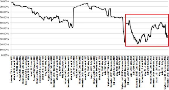
To calculate the data on the R software, the data was imported to the software. The data consists of 201 observations for both currencies. In the figüre 5, the correlation of the assests for 50 weeks have been demonstrated in a floating changeover graph in the regarding period. Except for the shocks in April 2005-2006 and November 2008-2009, the correlation between the two assests have decreased rapidly from 90% to 60%. Since January 2009, the correlation has been stuck in the band between 60% and 20% and does not show a distinctive tendency in this interim. The data used for the VAR calculation is the data belonging to the period between January 2009 and December 2012.
Figure 5: The graphic of the Dollar-Euro alteration correlation coefficient
After figuring out the changes in the corelations, the data has been started to be modified. If the marginals are to be , would be designated for the dollar returns and would be designated for Euro returns and w would be designated to stand for the portfolio weight. To form the portfolio, a “w” would be taken from the first marginal and a “1-w” would be taken from the second. The VAR of the portfolio has been calculated by the quantile command in the 5%, 10% and 1% shares. These percentages stand for the confidence level required to calculate the VAR values.
The VAR values have been calculated as below(R code): X1=Dolar ; X2=Euro
portföy=w*X1+(1-w)*X2
port.VAR=quantile(portföy,probs= “quantile”)
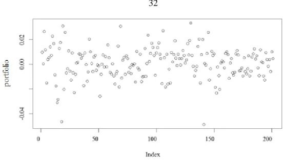
The distribution of the portfolio in the historical VAR context is as below(Figure 6):
Figure 6: The distribution of the portfolio prepared for the historical data 5.1.2. Maximum likelihood estimation
In the second method, the maximum likelihood method has been used. This method lies on the basis that the description of a probability distribution function of a variable is dependent on another parameter. The probability distribution function show us how frequent the dependent variable relies on the other parameter of interest (Kay, 1993).
The probability distribution function of a random X can be considered as ( ) ( ) and the can be considered to be a sample as an n unit taken from X’s distribution. The are independent and are distributive as X. The shared probability distribution function of the are
( )
( ) ( ) ( ) ( ) For the observed values of , the function above is to be a function of .
function is named the likelihood function. The value that maximizes this function is ̂( ) and the ̂( ) statistic is named as the maximum likelihood estimation. Generally, in order to calculate the maximum likelihood estimation of , the function “ln ( )L ”is maximized instead of “L( )”.
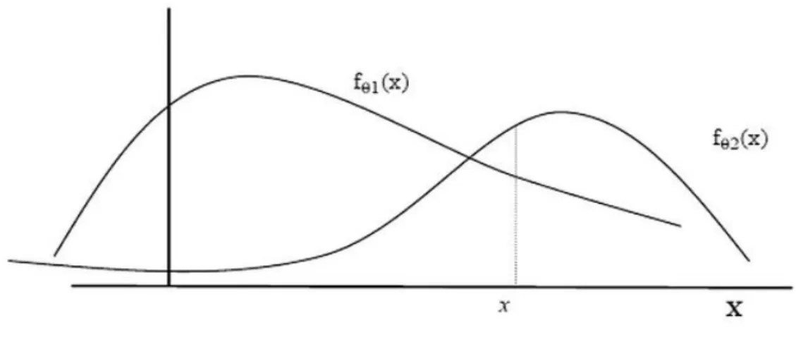
Let x be a random parameter and ( ) to be a distributive function dependent on x in the θ parameter. If the and , x is to have two possible values to get, the calculation done for is to get one distributive values that depend on and . For each calculation, ( ) and ( ) will get different values. The x value estimated for a calculation willl recieve x value when the calculation is applied on probability distributive functions. For instance, the predicted x parameter for the θ calculation mentioned in the Figure 7 is because the distribution of the probability function is greater in the calculation.
Figure 7: The x values recieves for maximum likelihood estimation method and marginals It has already been mentioned that the Dollar and Euro market indexes in hand belong to as marginal values. Each margin’s average is calculated by the “mean” command and their standard deviation is calculated by the “sd” command. In this method, in order to form the portfolio average and standard deviations have been used.
To produce the average p value in the first step; ( )
w value is the weight for the average p value, is the first marginal income average and is the second marginal income average.
Deviation value is calculated in the second step.
( ) ( ) ( ) ( ) ( ) w value is the weight for the average p value, is the first marginal income standard deviation, is the second marginal income standard deviation and ( ) states the two marginal income covariance value.
The “qnorm” command can directly calculate the value regarding the percentile. For instance, this can be done as qnorm(0.05)= -1.644854.
Calculated as the R value, the VAR value for maximum likelihood estimation is calculated by using the code below;
m.X1=mean(X1);m.X2=mean(X2);s.X1=sd(X1);s.X2=sd(X2) mu.p=w*m.X1+(1-w)*m.X2 sigma.p<-w^2*s.X1^2+((1-w)^2)*s.X2^2+2*w*(1-w)*cov(X1,X2) VAR95<-mu.p+qnorm(VAR)*sqrt(sigma.p) 5.1.3. Hull-White copula
In the third method, the Hull-White copula model has been used. This method is an interesting one, suggested by Hull-White (1998) to modal the multivariate distributions. This method shows that if the multivariate distributions do not distribute equally, the variance-covariance method can be used to equal the distributions and after this implementation the VAR values can be calculated by the usage of the Monte Carlo method.
Let it to be assumed that the are m numbered assests in the portfolio. An i numbered return-on-assests are to be and the function is to be the
return-on-assets distributions function of , the turn to the normal can assumed as the function in the is equal to the function.
( )
Here, N stands for the normal distributions function. While is standing for the percentile in the ( ) , stands for the equal percentile in standard normal distribution. This way, the that is counted as a return in the formula above, the normal standard normal is designated as . The original return value can be found when the replacement is made in the equation:
( )
The first formula enables the returns to become standard normal and the second formula enables the standard normal data to be transformed into the original data. The function can be turned into any form; for instance, there can be some heavy-tailed distributions or the function can be held equal to the empirical divison function that result from the original data. Then, let the transformed data be in the form. In this situation, the data divides as a normal multivariate and the average vector and the covariance matrix of the data can be estimated. As previously mentioned, Hull-White have offered to use the Monte Carlo method to simulate the return values of the normal standard distributions based on average and variance-covarience parameters. In return of the values that have ben simulated by using the second equation, the irregular values can be taken and the risk value can be predicted by the usage of the standard method. The nonparametric method that is based on the simulation seried can be held as an example for this case. This method is an uncomplicated one to use on a larger data series that consist of irregular variable distributions.
In this method, the maximum and minimum values have been decided on for the margins by assuming the margins are to be held on the ve variables . max.X1=max(X1);min.X1=min(X1);max.X2=max(X2);min.X2=min (X2)
Since the margins are assumed to be modal able in the [0,1] area of the copula using the maximum and the minimum values, the data are standartized.
t.X1=(X1-min.X1)/(max.X1-min.X1);t.X2=(X2-min.X2)/(max.X2-min.X2)
Later on, a mutual distributions function is decided on for each data. In this step, in order to prevent the maximum value to be equal to 1i the values equal to 1 have ben equalled to 0.999. If the maximum value is to be equalled to 1, in the latter steps the percentile functions returns infinite value.
e.X1=ecdf(t.X1)(t.X1);e.X1[e.X1==1]=0.999 e.X2=ecdf(t.X2)(t.X2);e.X2[e.X2==1]=0.999
The “ecdf” command that can be seen on the code helps to find the mutual distributions function. From the mutual distributions function, the percentile function can be found. The average of the percentile function is to be found. This process is done for each asset seperately.
f.X1=qnorm(e.X1);f.X2=qnorm(e.X2) m.X1=mean(f.X1);m.X2=mean(f.X2)
The found results are the empirical results that have been f.X1 standartized. The “mean” command has been used to find the average values of the emprical results. The values are to be put in order by using the “cbind” command and the covariance is found by using the the “VAR” command.
X1.X2=cbind(f.X1,f.X2) VC=VAR(X1.X2)
In order to form a copula after finding the covariance, a mutivariate distributions is made using the Monte Carlo method including the average and covariance forms.
f.X1.X2.dist=mvrnorm(MC,mu=c(m.X1,m.X2),Sigma=VC,empiri cal=TRUE)
In this formula, if “mvrnorm” shows the mutivariate distributions “mu” stands for average, “Sigma” stands for the covariance, “emprical” stands for emprical data, if it si not “TRUE”, the “FALSE” command is designated to get to the mutivariate distributions. Then, with the help of mutivariate distributions, two different probability function is to be formed.
e.X1.X2.dist.1=pnorm(f.X1.X2.dist[,1],mean=m.X1,sd=sd(f .X1))*(max.X1-min.X1)+min.X1
e.X1.X2.dist.2=pnorm(f.X1.X2.dist[,2],mean=m.X2,sd=sd(f .X2))*(max.X2-min.X2)+min.X2
The formed two distributions functions are taken to form the portfolio by taking a w weight from the first function and a 1-w weight from the second function. For the portfolio formed, the VAR values have been found by using the “quantile” command, as previously mentioned.
port.X1.X2=w*e.X1.X2.dist.1+(1-w)*e.X1.X2.dist.2 port.VAR=quantile(port.X1.X2,probs=VAR)
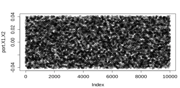
Here, the “probs” command stands for the confidence level. The portfolio that has been formed by the data and the required equations have been showed in Figure 8.
Figure 8: The distributions of the copula values that have been formed using the Hull-White method
5.1.4. Normal copula
The copulas, as mentioned previously, are studied under two titles that are the Eliptic copulas and the Archimedian copula family. The eliptic distributions are crucial distributions for the multivariate distributions because eliptic copulas have the features of the normal multivariate distributions. Moreover, multivariates permit to modal the extreme and irregular dependendy forms. Eliptic copula is a uncomplicated from of copula that consists of eliptic distributions. To provide simulations from eliptic distributions are easy to do and the most commonly used eliptic distributions are normal and student t distributions. The “MASS” and “copula” packages that are found ready in the R software plays an important role for the copulas to be modalled.
library("MASS") library("copula")
In the code with the “library” command the packages are made ready to be used in the software. The function code found ready in the packages helps to enable the code to be transformed to ant format.
0 2000 4000 6000 8000 10000 -0 .0 4 0 .0 0 0 .0 2 0 .0 4 Index p o rt .X1 .X2
In the forth method, the Gaussian (normal) copula method which is in the Eliptic copula has been used. This method is the simplest method to be applied on the copulas. To show the dependency form in the normal copula, the corelation parameter of the data-in-hand is used.
Correlation parameters show the direction and magnitude of the linear relationship between two random variables in statistics and probability theory. This coefficient vary between (-1) and (+1). Positive values show a direct linear relation, negative values show a reverse linear relation. If the correlation coefficient is 0, then there is no linear relation between the variables . Since the dependency between two assets are taken into account, it would be helpful during the modeling the correlation that shows deviancy from dependency. The correlation is obtained by dividing the variables ‘covariance to the product of the variables ’ standard deviation. The correlation coefficient is calculated by:
( )
“cov” is the covariance value, and is the standard deviation. The correlation can be fond via coding by:
cor(X1,X2)
The correlation parameter is very important for a normal copula. The relations between two-variable distributions are expressed with the correlation parameter. In simplest cases, this parameter is independent from the value of the variable and the distribution changes with the changing correlation parameter.
A normal copula consists of multivariate Gaussian distributions. If is the standard normal distribution, for (where is the correlation matrix) and the gaussian distribution is n-dimentional, the n-dimensional Gaussian Copula is expressed as:
( ) ( ( ) ( )) The density function is described as: