Third Triennial International Conference on Applied Automatic Systems Ohrid, Republic of Macedonia, September 18-20, 2003
AUTOMATED ASSEMBLY OF PRINTED CIRCUIT BOARDS: ITERATIVE SOLUTION OF PLACEMENT SEQUENCING AND FEEDER CONFIGURATION PROBLEMS
Ekrem Duman, Ahmet N. Ceranoglu
Dogus University, Department of Industrial Engineering Acibadem – Kadikoy, 34722 Istanbul, Republic of Turkey
Fax: +90 216 327 96 31
E-mail: [email protected]; [email protected]
Abstract: In automated assembly of printed circuit boards, the placement sequencing and feeder configuration problems turns out to be two of the four major problems that need to be solved efficiently to get better utilization from the use of computer controlled electronic component placement machines. The forms of these problems may show variability depending on the architecture of the placement machine used. In this study one of such machine architectures is undertaken where the most difficult combination of placement sequencing and feeder configuration problems is faced. Given a placement sequencing problem, the feeder configuration problem turns out to be a quadratic assignment problem, and given a feeder configuration the placement sequencing problem turns out to be a traveling salesman problem. However these two problems are highly interdependent and as the overall solution is intractable a sequential and iterative solution procedure is suggested. The proposed solution procedure is applied to test problems in real printed circuit board assembly environments. Copyright © 2003 Author and ETAI Society
Keywords: Printed Circuit Board Assembly, Placement Sequencing, Feeder Configuration
1. INTRODUCTION AND PROBLEM DEFINITION
Electronic component placement machines have become important productivity factors in the assembly of printed circuit boards (PCB), through their fast, error free and reliable component placement operations. However, some serious operations research problems arise through the use of these machines that need to be solved efficiently to get the highest utilization from these machines. The problems that may need to be solved in automated PCB assembly process can be classified into four classes similar to (Duman, 1998) as follows:
i. allocation of component types to machines (load balancing),
ii. determination of board production sequence, iii. feeder configuration,
iv. placement sequencing.
However, these four problem classes are interdependent, i.e. the solution of one affects the solution of others. Such an interdependency is more evident between the first two and the last two problems. Thus, if an optimal solution is desired, all four problems should be solved as a whole. However, in most cases, any one of these problems is NP-Complete and hence, trying to build and solve a monolithic model is intractable.
A general overview of PCB assembly problems is given by (McGinnis et.al. 1992; Ji and Wan, 2001). The formulations of the last two problems are mainly determined by the operating principles of the three moving parts that a typical placement machine has: i) Feeder Carriage; ii) Placement Head; iii) Carrier Board.
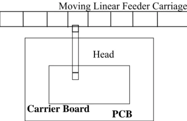
In this study a particular placement machine type which is depicted in figure 1 is undertaken. This
machine type leads to a complex and perhaps the most difficult combination of feeder configuration and placement sequencing problems. An example of this kind of machines is the Panasonic brand axial components placement machine.
Figure 1. Diagram of a numerically controlled component insertion machine.
The placement head is stationary, the carrier board is movable in two dimensions and aligns the placement location below the placement head. The feeder carriage is a linear cartridge one and it moves in one dimension to bring the component to be placed next in line with the placement head. Placement head picks up the component, moves down and makes the placement
The movement of the feeder carriage is not fast, and the time it takes for the desired cell to get aligned with the placement head depends to the position of the feeder carriage, which is defined by the identity of the previously placed component, and the proximity of the desired cell to the insertion head (naturally, a new insertion operation cannot start before the movement of the feeder carriage is completed).
The motions of the carrier board along the two axes are independent and at high speed. Nevertheless, since there are many placements on a single PCB and since a carrier board action is necessary before every placement, total distance traversed by the carrier board becomes important. This distance is directly related to the sequence with which components are placed on the PCB.
The placement head picks a component from the aligned feeder carriage cell and places it on the PCB set on the carrier board, which is aligned to enable placement to a precise location. The desired leg spread (span) or placement angle of components may be different, so, if necessary, the placement head adjusts the span and/or rotates before executing a placement. Afterwards, the component legs are cut to size and soldered to the PCB. Span adjustment is a slow operation and its duration depends on the
previous span setting of the placement head (i.e. the span of the previous component). Rotation can be made concurrently while the head moves down and needs no extra time. On the other hand, cutting and soldering operations do not take much time and are independent of component type.
On the other hand, the time passed between consecutive placements can not be less than a specific amount of time, called the free time, which is the time required by the placement head to move up and down. Together with the carrier board movement, feeder carriage and span adjustment times, the free time is an important determinant of the time passing between consecutive placements. For these type of machines, the placement sequencing and feeder configuration problems are highly interdependent. Feeder configuration influences the placement sequence since the time spent between two consecutive placements depends on the feeding time (thus, the feeder configuration) of the next component to be placed to the head. On the other hand, placement sequence influences the feeder configuration, since the amount (time) of linear feeder carriage movement depends on the distance between the feeder locations of the consecutively placed components (placement sequence).
Thus, if an overall optimal solution is desired, the two problems have to be handled and solved simultaneously. However, since the individual placement sequencing and feeder configuration problems lead to NP-Complete problems, building and solving such a monolithic model is almost intractable. Instead, in parallel to many other researches of similar problems (Duman, 1998; Grotzinger, 1992; Leipala, 1989), the problem is decomposed into two sub-problems (placement sequence and feeder configuration), and since they are interdependent, they are solved iteratively. That is, given a feeder configuration, the placement sequencing problem is solved and after that, for the obtained placement sequence, the feeder configuration problem is solved and the procedure is repeated until a predefined stopping condition is satisfied. This approach is called as the “decompose and iterate” methodology.
In the next section, the formulations of the associated TSP and QAP are given. The solution procedures proposed for the individual TSP and QAP are given in section three together with the structure of the TSP-QAP iterative solution procedure. The application of the solution procedure to test problems is discussed in section four and finally in section five, suggestions for future work are given.
Moving Linear Feeder Carriage
Carrier Board
PCB Head
2. PROBLEM FORMULATIONS
In the previous section, is was stated that, for a given feeder configuration, the placement sequencing problem can be formulated as a TSP and for a given placement sequence the feeder configuration problem can be formulated as a QAP. In the following subsections, the formulations of TSP and QAP adopted to our problem are given.
2.1. Placement Sequencing Problem Formulation For a given feeder configuration, the placement sequencing, can be modeled as a variant of the Traveling Salesman Problem (TSP) that has some minor differences from the classical TSP:
min
∑∑
= ≠ = N i N i j j ij ijx
t
1 1 (1) s.t.∑
≠ = N j i i ijx
1 = 1 jεN (2)∑
≠ = N i j j ijx
1 = 1 iεN (3)S
1
,−
≤
∑ ∑
∈S ∈ ≠ i j S j i ijx
for all S⊂
N (4) xij = 0 or 1 i, j = 1,..,N i≠
j whereN = set of all placement points
S = any non-empty proper subset of the set N xij = {1, if placement at point i precedes placement at
point j; 0, otherwise)
tij = time between the completion of consecutive
placements at points i and j
However, tij is not the frequently used Euclidian
distance (time), rather the Cheybshev distance (time) measure. That is, if,
t0 = component cut and clinch time,
t1
ij = carrier board movement time in x direction
between points i and j, t2
ij = carrier board movement time in y direction
between points i and j, t3
ij = span adjustment time if the spans of the
components placed at points i and j are different, t4
ij = time feeder needs to align component type of
placement at point j after point i,
t5 = free time (time between the head going up and
down),
then, tij turns out to be the following:
tij = t0 + maximum (t1ij, t2ij, t3ij, t4ij, t5) (5)
In many cases, the cut and clinch time denoted by t0
is quite small and independent of the component placement sequence, so it is usually dropped from the above expression.
2.2. Feeder Configuration Problem Formulation The formulation of the feeder configuration problem for a given placement sequence contains some non-linear terms. This non-non-linearity comes from the movement of the feeder carriage and the duration of bringing the component to be placed next depends on the feeder location of the previously placed component. That is, the cost (duration) of assigning a component type i to a feeder loacation j, depends also on where the other component types are assigned. This leads to a Quadratic Assignment Problem (QAP) formulation:
min ij kl I i j Jk I l J ijkl
x
x
c
∑∑∑∑
∈ ∈ ∈ ∈ (6) s.t.∑
∈I i ijx
= 1, jεJ (7)∑
∈I j ijx
= 1, iεI (8) xij = 0 or 1, iεI, jεJ where,I = set of component types J = set of feeder locations
cijkl = (feeder movement time from cell j to l) *
(the number of placements of component type i preceding the placements
of type k)
xij = {1, if component type i is assigned to
feeder location j; 0, otherwise}
The above QAP formulation assumes that the number of component types and the number of feeder cells are equal. If this is not the case, and the number of component types is larger, then it is necessary to assemble the PCB on two or more machines. This leads to a component allocation problem, which is discussed in (Duman and Duman, 2003).
On the other hand, if the number of feeder cells is larger, another complication arises. This complexity has two components. First, which component types should be assigned to more than one cell and which ones and second, from which cell should the component of a specific placement be picked up if that type of components are assigned to more than one cell (this complexity will not be handled within this study).
3. SOLUTION PROCEDURES DEPLOYED 3.1. TSP Solution Procedure
For the solution of the TSP, we used the Convex-Hull and the Or-Opt algorithms. The Convex-Convex-Hull algorithm was first proposed independently by Or (Or, 1976) and Stewart (Stewart, 1977). It is a heuristic procedure, which starts with a subtour consisting of the convex hull of all points to be visited. Then, at each iteration, a candidate point not on, but closest to the current subtour is determined and included into the subtour by eliminating the closest arc and connecting its endpoints to the candidate point. The details of the Convex-Hull algorithm can be found in (Or, 1976; Stewart, 1977). Starting with the solution found by the Convex-Hull algorithm, the Or-Opt procedure aims at improving a current tour by considering all possible relocations of every point, every two consecutive points and every three consecutive points along that tour (Or, 1976). The stepwise description of the Or-Opt implementation used in our study is as follows:
1. Starting with some first point in the given tour, consider all three consecutive points; temporarily remove them from the tour and consider inserting them in their normal order or reverse order between any two other consecutive points in the tour (while considering the point of insertion, start with the two points coming right after the removed three points and proceed clockwise). Make the first insertion that yields an improvement in tour cost permanent. Continue testing other three consecutive point exchanges until the start point is reached.
2. Repeat step 1 for all two consecutive point exchanges.
3. Repeat step 1 for every single point exchanges. According to the original work of Or (1976), there can be alternative strategies in the above procedure: In steps 1, 2 and 3, the insertion to be made permanent could be either the first one leading to a cost improvement, or, (after all possibilities being investigated) the one resulting in the highest cost improvement. Some experimentations have been accomplished to test the performance of both of these alternative strategies and the choice of accepting the first insertion leading to a cost improvement was found to be slightly superior and thus it is acted upon.
3.2. QAP Solution Procedure
The QAP in the context of PCB assembly optimization is studied in detail in (Duman and Or, 2003) where the performances of various exchange procedures and metaheuristic approaches (taboo search, simulated annealing and genetic algorithms)
are investigated. The best performing of those methods is a simulated annealing approach and thus, in this study we decided to implement it as the QAP solver in our TSP-QAP iterative solution procedure. A short description and the parameter settings of the simulated annealing procedure is given below: Simulated Annealing (SA) implements pairwise exchanges not only when they yield an improvement, but also (with a decreasing probability) when the objective value deteriorates. Thus, it opens the way to escape from local optima. The acceptance probability is set to e(- Δ/ T), where Δ is the deterioration level and T is a decreasing parameter (corresponding to Temperature in the analogy with physical annealing). In the beginning stages, T is high and pairwise exchanges with small deterioration are likely to be accepted (to avoid being prematurely trapped in a local optimum). As pairwise exchanges continue, T approaches zero and most uphill moves are rejected.
In the SA procedure used in this study, the following parameters are used:
i) Initial Temperature (T): The larger this value is, the more inferior exchanges are encouraged. It is set to 1000. For the real PCB problems considered in this study, T equaling 1000 approximately corresponds to accepting 10 per cent worse solutions by 0.75 probability.
ii) Temperature Decrease Ratio (a): After a predetermined number of iterations, T is set to T/a (i.e., T := T/a). When “a” is large, temperature decrease is faster and the acceptance of inferior exchanges is made less likely faster. According to numerical computations, a is set to 1.5.
iii) Number of Iterations at each temperature setting (R): Large values of R correspond to slower cooling; that is, more exchanges occurring when the acceptance likelihood of inferior exchanges are higher. The best value for R is determined to be 20.
iv) Increase Ratio in iteration number at each setting (b): After a predetermined number of iterations, R is set to R*b (i.e. R := R*b). In numerical computations, the suitable value of b is found to be 1.1.
v) Limit for the total number of iterations (Ite): There values for Ite (N3/3, N3 and 5/3*N3) are
experimented and N3 is decided to be the best.
3.3. TSP-QAP Iterative Solution Procedure
In fact, one may try to handle both feeder configuration and placement sequencing problems simultaneously and bring a solution to the combined problem. In this case, we have the feeling that, the meta-heuristic approaches (taboo search, simulated annealing and genetic algorithms) discussed in (Duman and Or, 2003) may show good performance.
However, because of the complexity that will arise even in the problem formulation, this kind of approach is not investigated within the scope of this study. Rather, we follow up the common approach in the literature as described below.
The QAP and the TSP problems should be solved iteratively since, the solution of the QAP influences the solution of the TSP and the solution of the TSP influences the solution of the QAP. This is because, the flow matrix, which is the most important input to the QAP, is determined by the solution of TSP, while changes in the TSP route influences and changes the optimal feeder (QAP) configuration. Similarly, in solving the TSP, the internode travel times are affected by the location of each component type in the feeder, which is determined by the QAP, and obviously a different TSP route can be obtained with a different feeder configuration.
An immediate question is when to stop iterations or how many times the QAP and the TSP has to be solved. The answer to this question is an important part of the iterative solution methodology. Below, the methodology developed and used in this study is described:
Step 0:
• Start with an arbitrary feeder configuration (or, in an application environment, the one being currently used);
• Solve the TSP using the current feeder configuration;
Calculate the TSP route cost and save it as the initial cost.
Step k (k
≥
1):• Update the flow matrix according to the current TSP route;
• (Starting with the current feeder configuration) solve the QAP using the current flow matrix;
Update the feeder configuration;
• Solve the TSP using the current feeder configuration;
Calculate the TSP route cost and save it as the current cost
If the stopping condition is met, stop; otherwise go to step k+1.
Stopping Condition:
Iteration number k reaching the predefined limit K or the current TSP cost being within ±r per cent of the TSP cost of the previous iteration. Note that, in the above methodology, the board assembly cycle time is exactly determined by the TSP route cost and thus, in determining the internode travel times, the actual values of machine parameters have to be used. On the other hand, the QAP is an
intermediate problem and the use of actual feeder speed values is not necessary.
4. EXPERIMENTATION
The methodology described in the previous section is applied to a nine problem data set adopted from boards data obtained from a TV sets manufacturing facility. For the machines populating these boards, the carrier board speeds in both x and y directions are determined as 20 cm/sec. The span adjustment speed is taken as 2 cm/sec (however, there are some board types for which the spans of all components are the same).
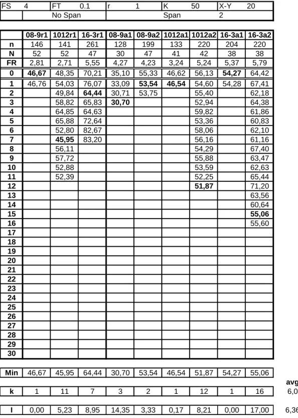
The iteration limit K and the stopping criterion r are taken as 50 and 1 per cent respectively in all runs. For the value of the feeder speed 4 cells/sec is taken. Free time (that is, the minimum possible time between two consecutive placements due to the physical actions involved) is taken as 0.1 sec. The initial feeder configuration is taken as the one currently being used in the facility. Full results of the runs are displayed in table 1, where the following abbreviations are used:
FS = feeder speed in cells/second. FT = free time in seconds.
r = termination criterion in percentage. K = iteration limit.
X-Y = carrier board x-y movement speed in cm/second.
Span = span adjustment speed in cm/second. n = number of components to be placed. N = number of component types. FR = average frequency ratio (n/N). Min = minimum TSP cost obtained. k = iteration number at termination.
I = improvement obtained with respect to initial TSP cost in percentage.
avg = average.
The experimentation base is not large enough to arrive at strong statistical results; however, a close inspection of table 1 leads to the following observations of interest:
1- Regarding all runs, the QAP-TSP iterative methodology is terminated in 6 iterations and 6.36 per cent improvement with respect to the initial solution, is attained. This improvement level is quite significant and shows the effectiveness of the methodology.
2- When span adjustment time is a critical problem parameter, larger improvements can be recorded. This is probably because, the span adjustment constitutes a second source of improvement besides the potential improvements regarding the feeder movements.
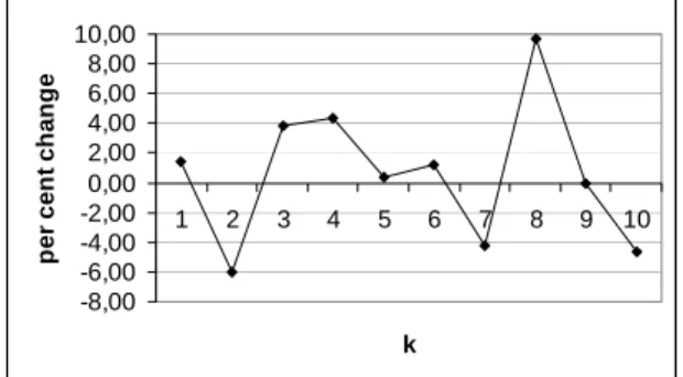
The behaviour of the TSP cost at each iteration is investigated in more detail. The iteration by iteration change in the TSP cost with respect to iteration number k is given in figure 2, where the numbers displayed are average of nine problems. We see that, in general, the procedure does not find better solutions at each iteration, but rather, it shows a random behaviour.
Figure 2. Iteration by Iteration Change in the TSP Cost.
A close inspection of table 1, reflects an important behaviour. Either, the procedure converges in a few number of iterations and there happens no significant change in the TSP cost, or the procedure continues for about ten iterations and the TSP cost fluctuates in significant amounts. With the given termination criterion (r = 1 per cent), the iteration limit (K = 50) is not reached at all. Rather, termination occurs in around 6 iterations and best solution is reached, on average, in 4.6 iterations.
5. CONCLUSION
The experimentations show that, the QAP-TSP iterative solution methodology usually terminates, on average, in 6 iterations and 6.36 per cent improvement is attained with respect to the initial solution. These results are obtained by taking the problem parameters FS = 4 cells/sec. and FT = 0.1 sec. The experimentation base should be enlarged to cope with other problem parameter settings and thus providing solutions to other placement machine types having this architecture.
The average 6.36 per cent improvement in board assembly time is quite significant and shows the importance of the QAP-TSP iterative solution methodology. Actually, if one is very keen for a better solution, the procedure can be implemented with smaller r (termination criterion) values, to search for some additional slight improvements in the solutions obtained.
The QAP-TSP iterative solution methodology described in this part may take a long time. For example, in the test problems, it took an average of 30 minutes (on a 166 MHz Pentium MMX computer) per QAP-TSP iteration in problems
having 50 component types and 200 placements, and as mentioned, there were, on average, 6 iterations per problem. However, since the requirement to solve such problems are not that frequent in real PCB assembly environments (may be once a day or even less), long run times do not cause a serious problem. In this study, one essential assumption made is that any component type would be assigned to a single cell in the feeder carriage. In real PCB assembly environments the number of feeder cells can be larger than the number of component types so that some of the component types can be assigned to more than one feeder cell. Such possibility may bring about a decrease in the total assembly time. However, in such a case the problem would become much more complicated but the effort deemed worthwhile and this is proposed as another future study area.
REFERENCES
Duman, E. (1998), Optimization Issues in Automated Assembly of Printed Circuit Boards. (PhD Dissertation), Department of Industrial Engineering, Bogazici University, Istanbul. Duman, E. and D. Duman (2003), Allocation of
Component Types to Machines in the Automated Assembly of Printed Circuit Boards, International Journal of Production Economics (submitted for publication).
Duman, E. and I. Or (2003), Quadratic Assignment Problem in the Context of Printed Circuit Board Assembly Process, European Journal of Operational Research (submitted for publication).
Grotzinger, S. (1992), Feeder Assignment Models for Concurrent Placement Machines. IIE Transactions 24, no. 4, pp. 31-47.
Ji, P., and F. F. Wan (2001), Planning for Printed Circuit Board Assembly: The State-of-the-art Review, International Journal of Compute Applications in Technology 14, iss. 4/5/6, pp. 136-144.
Leipala, T. and O. Nevalainen (1989), Optimization of the Movement of a Component Placement Machine, European Journal of Operational Research 38, pp. 167-177.
McGinnis, L. F., Ammons J. C., Carlyle M., Cranmer L., Depuy G. W., Ellis K. P. , Tovey C. A., Xu H. (1992), Automated Process Planning for Printed Circuit Card Assembly, IIE Transactions 24, pp. 18-29.
Or, İ., (1976), Traveling Salesman Type Combinatorial Problems and Their Relation to the Logistics of Blood Banking (PhD Thesis), Northwestern University.
Stewart, W. R. JR., (1977), A Computationally Efficient Heuristic for the Traveling Salesman Problem, In Proceedings of the 13th
Annual Meeting of S.E. TIMS, pp.75-85.
-8,00 -6,00 -4,00 -2,00 0,00 2,00 4,00 6,00 8,00 10,00 1 2 3 4 5 6 7 8 9 10 k pe r c e nt c h a n ge
Table 1. Iteration Based TSP Costs.
FS 4 FT 0.1 r 1 K 50 X-Y 20
No Span Span 2
08-9r1 1012r1 16-3r1 08-9a1 08-9a2 1012a1 1012a2 16-3a1 16-3a2
n 146 141 261 128 199 133 220 204 220 N 52 52 47 30 47 41 42 38 38 FR 2,81 2,71 5,55 4,27 4,23 3,24 5,24 5,37 5,79 0 46,67 48,35 70,21 35,10 55,33 46,62 56,13 54,27 64,42 1 46,76 54,03 76,07 33,09 53,54 46,54 54,60 54,28 67,41 2 49,84 64,44 30,71 53,75 55,40 62,18 3 58,82 65,83 30,70 52,94 64,38 4 64,85 64,63 59,82 61,86 5 65,88 72,64 53,36 60,83 6 52,80 82,67 58,06 62,10 7 45,95 83,20 56,16 61,16 8 56,11 54,29 67,40 9 57,72 55,88 63,47 10 52,88 53,59 62,63 11 52,39 52,25 65,44 12 51,87 71,20 13 63,56 14 60,64 15 55,06 16 55,60 17 18 19 20 21 22 23 24 25 26 27 28 29 30 Min 46,67 45,95 64,44 30,70 53,54 46,54 51,87 54,27 55,06 avg k 1 11 7 3 2 1 12 1 16 6,0 I 0,00 5,23 8,95 14,35 3,33 0,17 8,21 0,00 17,00 6,36